不可重复GRR研究
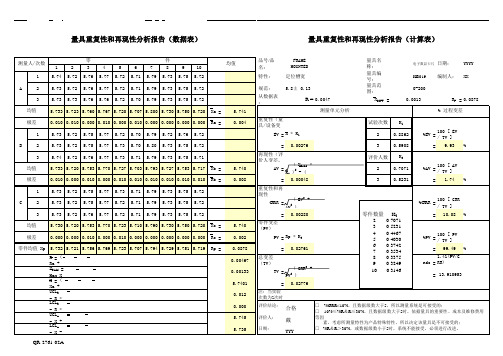
GRR卡尺重复性和再现性分析报告
0.000
0.000
0.000
0.000
0.000
0.000
0.000
0.000
0.000
0.000
0.000
0.000
0.000
0.000
0.000
0.000
0.000
0.000
0.000
0.000
0.000
0.000
0.000
0.000
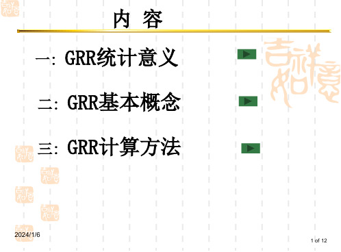
R-Chart
0.014 0.012 0.010 0.008 0.006 0.004 0.002 0.000
7
5.7933
8
5.7267
9
5.7533
10
5.7167
1
5.7300
2
5.7200
3
5.7533
4
5.7700
5
5.7233
6
5.7100
7
5.7900
8
5.7300
9
5.7500
10
5.7200
5.745
5.745
5.745
5.745
5.745
5.745
5.745
5.745
5.745
5.745
5.741 0.004
重复性(量具/设备变差,EV) EV = R * K1 = 0.00276
试验次数 2 3 评价人数 2 3
K1 0.8862 0.5908 K2 0.7071 0.5231 %AV = 100 [ AV / TV ] = 1.74 % %EV = 100 [ EV / TV ] = 9.93 %
0.012
0.012
0.012
grr指标 -回复
grr指标-回复GRR(Gage Repeatability and Reproducibility)指标是一个用于衡量测量工具可重复性和一致性的度量标准。
它是根据测量过程中的变异性来评估测量系统的准确性和稳定性。
GRR指标对于确保产品质量和提高生产效率至关重要。
本文将解释GRR指标的重要性,并提供一步一步的回答,以帮助读者更好地理解该指标。
第一步:介绍GRR指标GRR指标是用于评估测量系统的可重复性和一致性的一种统计分析方法。
它可以帮助生产商确定其测量系统是否足够准确,并能够精确地测量产品的特性。
GRR指标可以测量由于操作者、测量仪器或测量环境等因素引起的测量误差,并提供了改进测量系统以减少变异性的方法。
第二步:测量系统分析进行GRR分析的第一步是收集测量数据。
这些数据应包含来自不同操作者和不同时间点的重复测量。
收集的数据可以通过使用标准示例件(Master Parts)或参考值(Reference Values)来验证测量结果的准确性。
第三步:计算GRR指标计算GRR指标需要使用一种可行的统计方法,例如方差分析(Analysis of Variance,ANOVA)。
ANOVA可以将测量误差分解为以下三个主要来源:重复性误差(Repeatability Error)、操作者误差(Operator Error)和重复性操作者误差(Reproducibility Operator Error)。
通过计算这些误差的方差可以得到每个组件的测量系统的稳定性。
第四步:解释GRR结果通过分析GRR结果,可以确定测量系统的可接受性。
一般来说,可接受的GRR指标应小于或等于总变异性的10。
具体而言,重复性和操作者误差应小于于总变异性的5,而重复性操作者误差应小于总变异性的2。
如果GRR指标超过这些阈值,测量系统需要进行改进以提高其稳定性。
第五步:改进测量系统如果GRR指标超过了可接受的阈值,需要采取措施来改善测量系统的可靠性和准确性。
GRR目视系统与CPK制程能力指数

GRR目视系统与CPK制程能力指数GRR(Gauge Repeatability and Reproducibility)是一种评估测试设备的可重复性和再现性的方法,而CPK(Capability Process Index)是一种衡量制程能力的指标。
两者在质量管理中起着重要作用,并且经常同时使用。
GRR目视系统是一种测试设备,用于检测和记录产品特征的值。
它通常由一个操作员使用,通过目视观察来判断产品是否符合要求。
GRR目视系统的可重复性是指同一个操作员在相同条件下进行多次测试,得到相似结果的能力。
而再现性是指不同操作员在相同条件下进行测试,得到相似结果的能力。
通过进行GRR测试,可以评估目视系统的可靠性和稳定性,确保其能够准确地记录产品特征的值。
CPK制程能力指数用于衡量制程的稳定性和一致性。
它统计了制程的分布情况,比较了制程上限和下限与规范上限和下限之间的差异。
CPK指数越高,表示制程越稳定,能够产生符合规范要求的产品。
CPK制程能力指数是一种客观地判断制程是否稳定并且能够达到产品质量要求的方法。
GRR目视系统和CPK制程能力指数在质量管理中通常同时使用。
首先,通过进行GRR测试,评估测试设备的可重复性和再现性,确保测试结果的准确性。
然后,使用CPK制程能力指数来判断制程的稳定性和一致性,确保制造出的产品符合规范要求。
这两种方法互相补充,帮助企业提高产品质量,减少不良品率,并确保产品的一致性和可靠性。
总之,GRR目视系统和CPK制程能力指数是质量管理中两种重要的评估方法。
GRR目视系统评估测试设备的可重复性和再现性,CPK制程能力指数评估制程的稳定性和一致性。
两者的使用可以确保产品质量的一致性,并帮助企业提高生产效率和竞争力。
GRR(Gauge Repeatability and Reproducibility,即测量设备的重复性和再现性)和CPK(Capability Process Index,即制程能力指数)是两种在质量管理中常用的评估方法。
GRR测量系统分析报告范例
GRR测量系统分析报告范例一、引言GRR(Gage Repeatability and Reproducibility)是用来评估测量系统可重复性和一致性的方法。
该方法主要应用于检测设备的校准和评估,以确保测量结果的准确性和稳定性。
本报告旨在分析并评估测量系统的GRR。
二、实验目的本次实验的目的是评估测量设备所引入的测量误差和变异性,并确定该设备能否在溢出范围内提供一致准确的测量结果。
三、实验方法1.选择合适的测量设备:确保测量设备满足所需测量范围和准确性的要求。
2.根据测量需求,选择一组典型样本。
制定测量方案,包括测量次数和不同操作员的参与。
3.实施测量:根据测量方案要求,分别由不同操作员对样本进行多次测量。
4.数据收集:记录每次测量的数值,并整理成数据表格。
5.数据分析:使用GRR统计方法,对测量数据进行分析。
四、实验结果与讨论通过对测量数据进行分析,我们得到了以下结论:1. 测量设备的可重复性(Repeatability):根据GRR方法的定义,可重复性是指在同一操作员对样本进行多次测量时,测量结果的变异性。
可重复性通过测量系统内部误差来衡量。
经过分析,我们得到了测量设备的可重复性为X%。
根据测量标准的要求,此可重复性符合要求。
2. 测量设备的一致性(Reproducibility):一致性是指在不同操作员对同一样本进行测量时,测量结果之间的变异性。
一致性通过测量系统间误差来衡量。
经过分析,我们得到了测量设备的一致性为X%。
根据测量标准的要求,此一致性符合要求。
3.单次测量误差:通过计算测量系统的稳定性指标,我们得到了单次测量误差为X。
根据测量标准的要求,此误差在可接受范围内。
五、结论与建议根据我们对测量系统的分析,结合测量标准的要求,我们得出以下结论:1.所评估的测量系统的可重复性和一致性符合要求,能够满足预期的测量准确性和稳定性。
2.单次测量误差也在可接受的范围内。
3.根据实验结果,我们建议对测量系统进行定期的校准和维护,以确保其性能的稳定性和准确性。
GRR(重复性和再现性)简单介绍
MSA中GRR(重复性和再现性)简单介绍在日常生产中,我们经常根据获得的过程加工部件的测量数据去分析过程的状态、过程的能力和监控过程的变化;那么,怎么确保分析的结果是正确的呢?我们必须从两方面来保证,一是确保测量数据的准确性/质量,使用测量系统分析(MSA)方法对获得测量数据的测量系统进行评估;二是确保使用了合适的数据分析方法,如使用SPC工具、试验设计、方差分析、回归分析等。
测量系统的误差由稳定条件下运行的测量系统多次测量数据的统计特性:偏倚和方差来表征。
偏倚指测量数据相对于标准值的位置,包括测量系统的偏倚(Bias)、线性(Linearity)和稳定性(Stability);而方差指测量数据的分散程度,也称为测量系统的R&R,包括测量系统的重复性(Repeatability)和再现性(Reproducibility)。
01 引言一般来说,测量系统的分辨率应为获得测量参数的过程变差的十分之一。
测量系统的偏倚和线性由量具校准来确定。
测量系统的稳定性可由重复测量相同部件的同一质量特性的均值极差控制图来监控。
测量系统的重复性和再现性由Gage R&R研究来确定。
分析用的数据必须来自具有合适分辨率和测量系统误差的测量系统,否则,不管我们采用什么样的分析方法,最终都可能导致错误的分析结果。
在QS9000中,对测量系统的质量保证作出了相应的要求,要求企业有相关的程序来对测量系统的有效性进行验证。
02测量系统是用来对被测特性定量测量或定性评价的仪器或量具、标准、操作、方法、夹具、软件、人员、环境和假设的集合;用来获得测量结果的整个过程。
03表标准构成测量系统的主体元素之测量仪器必须经过校准至可追溯的标准国家标准←第一级标准(连接国家标准和私人公司、科研机构等)←第二级标准(从第一级标准传递到第二级标准)←工作标准(从第二级标准传递到工作标准)←量具04 术语4.1 分辨率:最小读数单位、测量分辨率、刻度限度或探测度。
测量系统分析---5 重复性和再现性 GRR

EV---Equipment Variation 设备变差----重复性: AV---Appraiser Variation 评价者变差---再现性: PV---Part Variation 零件的变差--------产品偏差:
与评价人之间的交互作用和由于量具造成的重复误差。但 计算复杂,需掌握一定程度的统计学知识。
-7-
第五章
重复性和再现性
GRR分析方法---极差法
例:2个评价人对5个零件进行测量。在研究中,两个评价人各将每 个零件测量一次。每个零件的极差是评价人A获得测量值和B获得 测量值之间的绝对差值。计算极差的和与平均极差。通过将平均极 差均值乘以1/d2*得到标准偏差.
计算A评价者测试数据的平均值 计算B评价者测试数据的平均值
计算C评价者测试数据的平均值 计算全部评价者所测数据的平均值 计算单个零件的平均值 计算零件全距Rp 计算最大与最小量测值班的差异 计算零件全距的极差R的平均值
-12-
6 7
8 9 10 11
=Max(Xa,Xb, Xc)-Min(Xa,Xb,Xc) =( Ra + Rb + Rc ) / 3
第五章
重复性和再现性
GRR分析方法
● 极差法 (全距法) 特点:简单快捷,能提供整体大概概况 ● 均值极差法(全距及平均值法)(包括控制图法) 特点:可将测量系统的变差分成两个部分-----重复性和再
现性,而不是他们的交互作用
● ANOVE法--方差分析法(变异数分析法) 特点:是一种标准统计技术,可算出零件、评价人、零件
GRR再现性和重复性
2024/1/6
8 of 12
3 GRR计算(二)
有3种方法:
➢ 极差法 (Range Method)
➢均值-极差法 (Average and Range Method
➢方差分析法
(ANOVA)
2024/1/6
9 of 12
量测系统的判定
GRR=<10% 量具系统可接受
可接受.可不接受,决定于该量具系
5 of 12
再生性(Reproducibility)
➢ 再生性又称作业者变异,指不同作业者以相同量具量测相同产品 的同一特性时,量测平均值的变异(3同一异)
➢ 在量测的条件有所变化下,重复的量测值之间的变异(操作者,装 夹,位置,环境条件,较长的时间段)
➢ 为外在因素引起的量测系统的变异
主值
检查员 A 检查员 B
内容 一: GRR统计意义 二: GRR基本概念 三: GRR计算方法
2024/1/6
1 of 12
1 GRR统計意义
➢ 测量系统变异概述
实际值
实际产品变异
实际值
测量值
量测系统
量测变异
量检具造成的变异 操作员造成的变异
观察到的产品变异
2024/1/6
2 of 12
测量系统精确度与准确度
准确度:平均值
2024/1/6
4 of 12
重复性(Repeatability)
➢ 重复性又称为量具变异,是指用同一种量具,同一位作业者, 多次量测相同零件的相同特性时的变异(四同)
➢ 在完全相同的量测条件下,多次量测值间的差异
➢ 为量测系统本身产生的差异,随机误差范畴
良好重复性
主值
主值
GRR再现性和重复性

量测系统分析 Gauge Repeatability and Reproducibility
2019/5/3
1 of 12
内容 一: GRR统计意义 二: GRR基本概念 三: GRR计算方法
2019/5/3
2 of 12
1 GRR统計意义
测量系统变异概述
实际值
实际产品变异
实际值
测量值
可接受.可不接受,决定于该量具系
10%<GRR<30% 统之重要性,修理所需之费用等因
素
GRR>=30%
量具系统不能接受, 须予以改进
2019/5/3
11 of 12
2019/5/3
12 of 12
总变异:TV TV = GR&R 2+ PV 2
2019/5/3
9 of 12
3 GRR计算(二)
有3种方法:
极差法 (Range Method)
均值-极差法 (Average and Range Method
方差分析法
(ANOVA)
2019/5/3
10 of 12
量测系统的判定
GRR=<10% 量具系统可接受
精确度:变动性 观察到的变动性 = 产品变动 + 衡量的变动
实际值
测量值
2 总量
=
2 产品
+
2 测量
衡量系统变动性- 通过 “GR&R 研究”决定
2019/5/3
5 of 12
重复性(Repeatability)
重复性又称为量具变异,是指用同一种量具,同一位作业者, 多次量测相同零件的相同特性时的变异(四同)
- 1、下载文档前请自行甄别文档内容的完整性,平台不提供额外的编辑、内容补充、找答案等附加服务。
- 2、"仅部分预览"的文档,不可在线预览部分如存在完整性等问题,可反馈申请退款(可完整预览的文档不适用该条件!)。
- 3、如文档侵犯您的权益,请联系客服反馈,我们会尽快为您处理(人工客服工作时间:9:00-18:30)。
NON-REPLICABLE GRR CASE STUDY David Benham, DaimlerChrysler Corporationwith input from the MSA workgroup:Peter Cvetkovski, Ford Motor CompanyMichael Down, General Motors CorporationGregory Gruska, The Third Generation, Inc.ABSTRACTGage studies provide an estimate of how much of the observed process variation is due to measurement system variation. This is typically done by a methodical procedure of measuring, then re-measuring the same parts by different appraisers. This cannot be done with a non-replicable (destructive) measurement system because the measurement procedure cannot be replicated on a given part after it has been destroyed. Here a method using ANOVA is used in a case study which demonstrates one possible way to determine measurement variation in a non-replicable system.This paper is intended to serve as additional guidelines for the analysis of measurement systems.Non-Replicable GRR Case StudyGage studies provide an estimate of how much of the observed processvariation is due to measurement system variation. This is typically doneby a methodical procedure of measuring, then re-measuring the sameparts by different appraisers. With a standard 10-3-31GRR, anassumption is made that between the trials and when handing offbetween appraisers, no physical change has occurred to the part. Allappraisers in the study have the opportunity to examine the same parts.The measurements can be replicated between appraisers and betweentrials. With most situations this is a safe assumption to make.In Figure 1, there are 10 parts to be measured, numbered from 1 to 10.As can be seen, the same part is measured by each appraiser and for eachtrial. A 10-2-3 format is shown for the sake of brevity and as a lead-in tothe case study which follows; randomization is not shown for the sake ofclarity.Appraiser 1 Appraiser 2Part # Trial 1 Trial 2 Trial 3 Trial 1 Trial 2 Trial 31 1 1 1 1 1 12 2 2 2 2 2 23 3 3 3 3 3 34 4 4 4 4 4 45 5 5 5 5 5 56 6 6 6 6 6 67 7 7 7 7 7 78 8 8 8 8 8 89 9 9 9 9 9 910 10 10 10 10 10 10Figure 1: Example of a Standard GRR Layout (10-2-3)However, there are certain instances where the measurements cannot bereplicated between trials or appraisers. The part is destroyed orsomehow physically changed when it is measured – that characteristiccannot be measured again. That measurement characteristic is said to benon-replicable. An example might be a destructive weld test where aweld nut is pushed off a part and the peak amount of pushout forcebefore destruction is measured; the weld is destroyed in the process, so itcannot be measured again. So, how can a measurement systems analysisbe conducted when the part is destroyed2 during its measurement?110 parts, 3 appraisers, 3 trials.2Not all non-replicable MSA studies necessarily involve destroying parts. In fact, the measurands need not be parts per se, either. For example, when tests are done on chemical processes, the chemical sample (“part”) used for testing may have been altered by the test itself and the solution it was drawn from may have been from a dynamic process where the solution is in constant motion – therefore it cannot be precisely re-sampled.Non-Replicable GRR Case StudyJune 5, 2002The first thing that must be done before tackling a non-replicable GRR study is to ensure that all the conditions surrounding the measurement testing atmosphere are defined, standardized and controlled – appraisers should be similarly qualified and trained, lighting should be adequate and consistently controlled, work instructions should be detailed and operationally defined, environmental conditions should be controlled to an adequate degree, equipment should be properly maintained and calibrated, failure modes understood, etc. Figure 2 in the MSA manual, Measurement System Variability Cause and Effect Diagram, p. 15, and the Suggested Elements for a Measurement System Development Checklist, pp. 36 – 38, may assist in this endeavor. Second, there is a good deal of prerequisite work that must be done before doing a non-replicable study. The production process must be stable and the nature of its variation understood to the extent that units may be appropriately sampled for the non-replicable study – where is the process homogeneous and where is it heterogeneous? Another consideration: if the overall process appears to be stable AND CAPABLE, and all the surrounding pre-requisites have been met, it may not make sense to spend the effort to do a non-replicable study since the overall capability includes measurement error – if the total product variation and location is OK, the measurement system may be considered acceptable. Standard GRR procedures and analysis methods must be changed and certain other assumptions must be made before conducting a non-replicable measurement systems analysis. The plan for sampling parts to be used in a non-replicable GRR needs some structure. Since the original part cannot be re-measured due to its destruction, other similar (homogeneous) parts must be chosen for the study (for the other trials and other appraisers) and an assumption must be made that they are “duplicate” or identical parts. In other words, as the “duplicate” parts are re-measured across other trials and by other appraisers, we will pretend that the same part is being measured. Refer to Figure 2. “Part 1” is now Part 1-1, 1-2, 1-3, 1-4, 1-5, 1-6, for this 10-2-3 layout. Six very similar, assumed to be identical, parts are used to represent Part 1, and so on for all 10 parts. The assumption must be made that all the parts sampled consecutively (within one batch) are identical enough that they can be treated as if they are the same. If the particular process of interest does not satisfy this assumption, this method will not work .Non-Replicable GRR Case StudyJune 5, 2002Appraiser 1 Appraiser 2Part # Trial 1 Trial 2 Trial 3 Trial 1 Trial 2 Trial 31A…1F 1-1 1-2 1-3 1-4 1-5 1-62A…2F 2-1 2-2 2-3 2-4 2-5 2-63A…3F 3-1 3-2 3-3 3-4 3-5 3-64A…4F 4-1 4-2 4-3 4-4 4-5 4-65A…5F 5-1 5-2 5-3 5-4 5-5 5-66A…6F 6-1 6-2 6-3 6-4 6-5 6-67A…7F 7-1 7-2 7-3 7-4 7-5 7-68A…8F 8-1 8-2 8-3 8-4 8-5 8-69A…9F 9-1 9-2 9-3 9-4 9-5 9-610A…10F 10-1 10-2 10-3 10-4 10-5 10-6Figure 2: Non-Replicable GRR Layout3Care must be taken in choosing these “duplicate” parts. Typically for theparts that represent part number 1 in a study, each “duplicate” is selectedin a way that it is as much alike the original part as possible. Likewisefor part number 2, and number 3, 4, 5, etc. These parts should beproduced under production conditions as similar as possible. Considerthe “5 M’s +E”4 and make them all as alike as possible. Generally, ifparts are taken from production in a consecutive manner, thisrequirement is met.However, the parts chosen to represent part number 2, for example, mustbe chosen to be unlike part number 1, part number 3, 4, 5, etc. Sobetween part numbers, the 5 M’s +E must be unlike each other. Thesedifferences must be forced to be between part numbers. The totalnumber of duplicate parts selected for each row must equal the numberof appraisers times the number of trials.5 In Figure 2, groups of partswithin each row are assumed to be identical, but groups of parts betweenrows are assumed to be different.Part variation may be expressed as part-to-part, shift-to-shift, day-to-day,lot-to-lot, batch-to-batch, week-to-week, etc. With parts the minimumvariation would be part-to-part – this represents the minimum possibleamount of time between each part. When parts are not sampledconsecutively (i.e., part-to-part), there is more opportunity for variationto occur – different production operators, different raw material, differentcomponents, changes in environment, etc.So, within a row it is desirable to minimize variation by taking partsconsecutively, thus representing part-to-part variation. Between rows itis desirable to maximize variation by taking parts from different lots,batches, etc. There may be economic, time or other constraints involvedwhich will impose limits on the length of time we can wait to take3The necessary randomized presentation to the appraiser is not shown here for the sake of clarity.4Man, Machine, Material, Method, Measurement plus Environment. Measurement may seem redundant here, but there may be times where two or more “identical” measurement systems are used to gain the same information and this should be considered in any study.5When the source of measurement variation is thought to be due to equipment only, using different appraisers may not be required.Non-Replicable GRR Case StudyJune 5, 2002samples for the between-row data – the process must be run, the PPAPmust be submitted, etc. When constraints arise and interfere with doingthings the “right” way, the results may be subject to modifiedinterpretation.Another statistical assumption that must be made for this type of study isthat the measurement error is normally distributed. This is a prerequisitefor any ANOVA (Analysis of Variance).ANOVA is a better analysis tool for a non-replicable measurementsystems analysis than the average and range method. ANOVA has thepower to examine interactions that the average range method will notcatch.As a precautionary note, the results from this type of study willcontain some process variation because the “identical” parts arenot really identical. This may come into play when interpreting theresults in terms of the error percentage related to process variationor tolerance. The better the methodology used to achieve anunderstanding of the production process and its correspondingmeasurement system, the more meaningful this non-replicablemeasurement study will be.It is critical in a non-replicable GRR study that the parts be clearlyidentified and saved after testing. If any issues arise after the standardanalysis, these parts may be needed for further exploration – e.g.,microscopic examination.A case study may serve to better illustrate this methodology.CASE STUDYA stamped part goes through a critical weld assembly process whichmust be destructively tested on an ongoing basis. The process has an in-house progressive stamping die which produces the steel stampings.This process is followed by robotic MIG welding (attaching an outsidepurchased steel rod to the stamping) in one of 6 different weld stationseach of which has 4 parallel weld fixtures (only one of which will beused per assembly). Each weld fixture is assigned a letter designation, Athrough X. This process has been in production long enough that it hasbeen studied and analyzed for stability and capability. Each of the 24weld stations is providing a stable and capable process, however someare better than others. In an effort to improve the overall process, themeasurement system would be analyzed using this non-replicable MSAmethodology which had been recently introduced to the supplier.This study used the 10-2-3 format – 10 parts, 2 appraisers, 3 – thus Study Formatrequiring 60 parts total for the study. Given the complexity of theprocess, it was felt that the 10-2-3 would be more manageable than a 10-3-3. Although there are 24 weld fixtures, only 10 of them were used forthis study and they were chosen using previously gathered data toNon-Replicable GRR Case StudyJune 5, 2002 represent the full range of the process. There was enough earlyconfidence in the measurement system to make this judgment.Similarity (homogeneity) within each row was created by taking 6consecutively produced stampings (6 is chosen to meet the 2 appraisers x3 trials requirement), then welding those 6 parts consecutively throughthe same weld fixture. Dissimilarity (heterogeneity) between rows wascreated by taking groups of 6 consecutive stampings from different coilsof steel at a time separated by a few hours, then running themconsecutively through a different weld fixture at a different time.The rod component which is welded to the stamping is received in bulkand has already been determined to not play a major role in pull testvariation. Therefore, in this study there was no effort made to maintainsimilarity and dissimilarity issues with the rod component.Previous studies using common problem solving tools had shown that amanual positioning and clamping system used on the testing machinewas appraiser dependent, so a new and better positioning system withhydraulic clamps was installed. Parts are located into the machine withpositive locators and hydraulic clamps. A hook on the testing machinegrabs the rod and mechanically pulls on the rod to destruction. A digitalreadout on the machine displays the peak pulloff force in pounds andreads to one decimal place. From this readout, the data is recorded andthe failure mode noted (weld must pull metal from the stamping).Although the appraiser dependency was assumed to be resolved, thisstudy still used two appraisers to verify that assumption.A total of 60 parts were required to do this study. There were 10 groupsof similar parts, 2 appraisers and 3 trials; 10 x 2 x 3 = 60. Parts werefirst gathered off the stamping operation, carefully numbered andquarantined until all 60 parts had been collected. These 10 groups ofparts were selected at 3 hour intervals, over 3 days of production, inorder to force some difference between each group of parts.Then, each similar stamped group of parts was run through a differentweld fixture. Parts introduced to each weld fixture were presented inrandom order within each group of 6.Appraiser 1 Appraiser 2Part # Trial 1 Trial 2 Trial 3 Trial 1 Trial 2 Trial 31-1R…1-6R 1-6R531-5R251-3R71-4R401-1R341-2R322-1P…2-6P 2-2P272-6P352-5P572-4P122-3P432-1P173-1H…3-6H 3-1H213-2H363-6H13-5H563-4H103-3H264-1G…4-6G 4-4G464-6G424-3G84-2G284-1G554-5G305-1E…5-6E 5-4E55-3E205-1E135-6E545-2E395-5E506-1F…6-6F 6-1F526-3F36-4F376-5F296-2F516-6F457-1M…7-6M 7-6M167-4M117-1M237-2M67-3M157-5M148-1O…8-6O 8-6O498-3O608-1O338-5O418-2O448-4O199-1Q…9-6Q 9-5Q319-6Q599-3Q249-2Q49-4Q99-1Q210-1T…10-6T 10-2T2210-5T1810-3T4710-4T5810-1T4810-6T38Figure 3: Layout Used for Case StudyNon-Replicable GRR Case StudyJune 5, 2002Referring to Figure 3, each row shows the “similar” parts. “1-1R” standsfor Stamping #1 of the first group of 6 stampings, which was run throughweld fixture R. “1-2R” stands for Stamping #2 of the first group ofstampings, which was run through weld fixture R. “10-1T” stands forStamping #1 of the tenth group of stampings, which was run throughweld fixture T.6The parts were numbered with the identification shown in Figure 3.Parts within each row were presented in a random order to both the weldassembly operation and to the weld test operation, each with a differentrandom order. The order shown above is for the weld test operation; theorder for the weld assembly operation within each row was a differentrandom order and is not shown here. Such randomization reduces thepossibility of any bias present in the order of manufacturing and/ortesting.Once all assembly was completed, the parts were presented to theappraisers for destructive testing and the data were recorded. Parts weresaved, preserving the original part numbers, in case any post-analysisneeded to be done.RESULTSThe data were put into a Minitab® “Gage R&R (nested)” routine whichgenerated a nested ANOVA. A nested (vs. crossed) ANOVA is requiredfor this type of study because all parts are not tested by (crossed with) allappraisers across all trials – they cannot be because they are destroyedafter one test. Each appraiser cannot be crossed with each part. Othercharts were also generated by Minitab.The first thing to look at is the Gage Run Chart.6For the sake of clarity here, the randomized order of total presentation to the appraisers running the test machine is shown as a subscript.Non-Replicable GRR Case StudyJune 5, 2002Figure 4: Gage Run Chart – Weld Tester, Rod PulloffThe Gage Run Chart in Figure 4 shows plotted points that representindividual measurement values made on each “part” by each appraiserduring each trial. The data is grouped by appraiser and presented in theorder in which the trials occurred. The horizontal dashed line representsthe overall mean of all the individual values displayed on the chart. Theabscissa shows each “part” number (a group of 6 parts in this case).This type of chart provides visual clues as to the presence of any patternsin the data. It is desirable that there be no particular pattern within“parts.” If undesirable patterns are present, then further, moresophisticated investigation may be required. It is also desirable that therebe differences shown between “parts”. If these differences do not occurthen the measurement system cannot distinguish between the parts usedin the study. Since there are no control limits or other statistical guidesdisplayed on this chart, some guesswork and common sense may berequired when reviewing it.In this particular study, there are no significant patterns within “parts”and there is some difference between “parts.”Next the summary of the GRR graphics is reviewed.Non-Replicable GRR Case StudyJune 5, 2002Figure 5: GRR Summary Graphics – GRR Study (Nested), Weld Tester, Rod PulloffA graphical summary, generated by Minitab, of this study is presented inFigure 5. Five graphs are shown and are numbered from 1 to 5.Presentation and analysis of these charts falls in line with a standardGRR.Graph No. 1 shows the components of variation. Four sources aredisplayed here• Gage R&R – is the variation due to the measurement system.• Repeatability – is the variation due to the measuring equipment.• Reproducibility – is the variation due to differences in the appraisers.• Part-to-Part – is the variation due to measurements taken acrossdifferent parts.Two bars are shown for each source of variation7:• % Contribution – is 100 times that variance component sourceσ).divided by the total variance (2• % Study Variation – is 100 times that study variation source dividedby the total study variation (σ).7It is possible in Minitab to also display “% Tolerance” and “% Process” but these options were not chosen here.Non-Replicable GRR Case StudyJune 5, 2002Graph No. 2 is a Range (R) Chart showing the range of the readings foreach appraiser on each “part.” Note that there is an upper control limit(UCL) and lower control limit (LCL) and that to be acceptable all pointsshould be within these limits. Out of control conditions means there issome sort of inconsistency occurring and should be investigated beforegoing further.The data in this case study is all within the control limits and isconsidered acceptable with respect to the Range Chart.Graph No. 3 is an Xbar (X) Chart showing the average of eachappraiser’s 3 readings on each “part.” Note that there is an upper controllimit (UCL) and lower control limit (LCL) and that to be acceptable,approximately 50% of the points should be outside these control limits.The distance between the control limits represents the band ofmeasurement system variation. If all points were within the controllimits it would mean that no significant distinction can be made betweenany of the parts in the study.In the data for this case study, 11 of 20 points (55%) are out of controland this is considered acceptable for the Xbar Chart.Graph No. 4 is a chart of the part-to-part variation across the study. Forthis particular study, Graph 4 does not add much value.Graph No. 5 shows the grand average for each appraiser as well aspoints representing the individual readings. The horizontal line betweenthese points indicates a visual reference for the difference in the grandaverage – the flatter this line the less difference there is between thesegrand averages.In the data for this case study, the reference line is quite flat indicatingvery little difference in the grand average for each appraiser.Graphs 4 and 5 may be used as clue generators for further analysis.Also, other graphics, such as histograms, may be used for more detailedanalysis.While reviewing the graphics it is a good idea to at the same time reviewthe ANOVA summary of the GRR data. Again, this summary is thesame as a standard ANOVA table and what would be generated by astandard GRR study.Gage R&R Study - Nested ANOVANested ANOVA TableSOURCE DF SS MS F PAppraiser 1 15636 15636 0.0202 0.88869Part(Appraiser) 18 13965615775868 16.7447 0 Repeatability 40 1853410 46335Total 5915834661Non-Replicable GRR Case StudyJune 5, 2002Gage R&RSOURCE VARCOMP % CONTRIBUTION(OF VARCOMP)Total Gage R&R 46335 16.00 Repeatability 46335 16.00 Reproducibility 0 0 Part-To-Part 243177 84.00 Total Variation 289513 100.00SOURCE STD DEVIATION(SD) STUDY VARIATION(6 * SD)% STUDY VARIATION(% SV)Total Gage R&R 215.256 1291.54 40.01Repeatability 215.256 1291.54 40.01Reproducibility 0 0 0Part-To-Part 493.130 2958.78 91.65Total Variation 538.064 3228.38 100.00Given all the above information one must make some decisions about themeasurement system – is it acceptable, is it useable, is more studyneeded, does an appraiser need better training, is customer approvalrequired for use, etc? For acceptability, generally the GRR% is reviewedfor suitability8.In this particular case study example the overall GRR% = 40.01% whichdoes not make for a clean interpretation. Is this acceptable given that thetraditional upper limit for even a marginally acceptable measurementsystem is 30%?Consider:1. The overall process to which the GRR% is compared is actuallyrepresented only by the parts (and weld fixtures) chosen for thisstudy. Only 10 of the 24 weld fixtures were included in thisstudy. Not all of the process is necessarily represented here. Ifthe process variation due to all the fixtures is much larger thanthat of the 10 selected for this study, then the measurementsystem may be acceptable based on MSA guidelines.2. The data in any non-replicable study such as this will necessarilyinclude SOME process variation. So some portion of the 40.01GRR% is actually process variation. It is impossible to separateall process variation from measurement system variation withthis scheme.3. The machine used to do the destruct pulloffs is a relativelysophisticated and expensive piece of equipment. How much 8ndc is also typically reviewed at this time, however for the sake of brevity it will not be shown here.Non-Replicable GRR Case StudyJune 5, 2002more could it be improved and would it be cost effective? Thesewould be questions for a possible cost study.Determining the acceptability of results of a non-replicable study Acceptability Issuesinvolves many other possible issues which go beyond the immediatesubject of this paper.• Production process stability: In order to properly analyze andinterpret a non-replicable measurement system study, the productionprocess must be statistically stable. Since the measurement systemstability is contained within the production process data, if theoverall data demonstrates stability, then the measurement system istheoretically stable. Data collection frequency and sample size mustbe balanced between Average Run Length (ARL)9 and cost ofinspection.• Production process capability: If the production process ismarginally capable, there is not much breathing room between itsnatural process limit(s) and the measurement system’s “gray area”(see discussion in Chapter III, Section C, of MSA-3). Acceptabilitylimits (for the process data) might be used when the non-replicablemeasurement system analysis shows marginal or questionableacceptability. These acceptability limits would be calculated byσ, then adding that valueusing a 3 or 4 sigma multiplier10 of theGRRto the lower specification limit and subtracting it from the upperspecification limit. However, for this to work with any degree ofconfidence, there must be adequate breathing room between theproduction process and these limits. In the example provided, wherethere is only a lower specification limit, the resultant value fromusing this multiplier would be added to the lower specification limitonly; for a process with only an upper specification limit, theresultant value from using the multiplier would be subtracted fromthe upper specification limit only.• Long-term measurement system stability: Some effort should bemade to study the measurement system’s stability on a long-termbasis using techniques similar to what has been described above.These techniques may be scaled down to “mini” studies and used onan ongoing basis.• Ironically, the better the process Cp11, the more difficult it may be toestablish acceptable non-replicable measurement system analysisresults using the methods here. Recall that a major requirement forthis method to work successfully is that one can knowingly producesimilar (homogeneous) parts (to be used within “parts” and operatoracross trials) and dissimilar (heterogeneous) parts (to be usedbetween “parts” and operators). If the production process has a very9The average run length (ARL) at a given quality level is the average number of samples (subgroups) taken before an action signal is given.10This multiplier value would be chosen depending on the amount of risk one chooses to accept.11Technically a process with unilateral tolerance (such as demonstrated in the case study here) has no Cp. What is meant here is a process with a relatively small amount of variation.Non-Replicable GRR Case StudyJune 5, 2002tight Cp, it may not be possible to meet this requirement. However,if such a process were to demonstrate stability and a high Cpk, thenthe measurement system is probably acceptable (provided there areno bias or linearity issues) because the data that generated this highCpk would include measurement variation.• Bias and linearity are not evaluated by this method. As with anyGRR study, only repeatability and reproducibility are considered.The measurement equipment calibration plan becomes critical to theoverall acceptability of the non-replicable measurement system.As can be seen, a non-replicable measurement study may raise as many Summaryquestions as it resolves. Due to the relative sophistication and expense ofthe measurement equipment used in this non-replicable measurementprocess, and due to the factors mentioned above, it was decided that thismeasurement process was suitable for gaging continuous improvement ofthe manufacturing process. At the same time, opportunities forimproving the measurement system would also be evaluated in thefuture.This case study is a single event and therefore has been termed a non-replicable GRR study. The bigger picture with any measurement systemis the long-term, cradle-to-grave concept. The study here may be used toinitially qualify a system, but more work is required to control thatmeasurement system over time to ensure its stability and usefulness inmaking the appropriate process control and/or capability decisions andcontinuous improvement. To keep tabs on this measurement process overtime, a control chart could be used to record the results of special,consecutive samples taken periodically and those results used todetermine the system’s stability.Finally, the methodology above was what was chosen for this particularsituation. There are other methods which will serve to determine non-replicable measurement error and each must be carefully selected to suitthe particular situation. The methods shown here merely illustrate asingle approach for a single situation and hopefully it will spur the readerto consider developing an approach for their own non-replicablemeasurement error situation._____________________________________________________________________________________________Dave Benham works at DaimlerChrysler Corporation in Auburn Hills, Michigan, as a Senior Consultant in Supplier Development. He has a B.S. in Psychology and M.A. in Education from Michigan State University. Dave is an ASQ Certified Quality Engineer and Certified Reliability Engineer. He has worked in the automotive industry in the field of quality for 25 years.。