Poisson and normal

合集下载

概率论中几种具有可加性的分布及其关系

概率论中几种具有可加性的分布及其关系目录摘要 (1)关键词 (1)Abstract (1)Key words (1)引言 (1)1 几种常见的具有可加性的分布 (1)1、1 二项分布 (2)1、2 泊松分布(Possion分布) (3)1、3 正态分布 (4)1、4 伽玛分布 (6)1、5 柯西分布 (7)1、6 卡方分布 (7)2 具有可加性的概率分布间的关系 (8)2、1 二项分布的泊松近似 (8)2、2 二项分布的正态近似 (9)2、3 正态分布与泊松分布间的关系 (10)2、4 正态分布与柯西分布、卡方分布及卡方分布与伽玛分布的关系 (11)3 小结 (12)参考文献 (12)致谢 (13)概率论中几种具有可加性的分布及其关系摘要概率论与数理统计中概率分布的可加性就是一个十分重要的内容、所谓分布的可加性指的就是同一类分布的独立随机变量与的分布仍属于此类分布、结合其特点,这里给出了概率论中几种具有可加性的分布:二项分布,泊松分布,正态分布,柯西分布,卡方分布以及伽玛分布、文章讨论了各类分布的性质及其可加性的证明,这里给出了证明分布可加性的两种方法,即利用卷积公式与随机变量的特征函数、除此之外,文章就可加性分布之间的各种关系,如二项分布的泊松近似,棣莫佛-拉普拉斯中心极限定理等,进行了不同层次的讨论、关键词概率分布可加性相互独立特征函数Several Kinds of Probability Dstribution and its Relationshipwith AdditiveAbstract Probability and mathematical statistics in the probability distribution of additivity is a very important content 、The distribution of the so-called additivity refers to the distribution of thesame kind of independent random variables and distribution are still belong to this kind ofdistribution 、Combined with its characteristics, here given several has additivity distribution in probability theory: the binomial distribution, poisson distribution and normal distribution andcauchy distribution, chi-square distribution and gamma distribution 、Article discusses the nature of all kinds of distribution and its proof of additivity, additive of proof distribution are also given two methods, namely using convolution formula and characteristic function of a random variable 、 In addition, this paper the relationships between the additive property distribution, such as thebinomial distribution of poisson approximation, Di mo - Laplace's central limit theorem, and so on,has carried on the different levels of discussion 、Key Words probability distribution additivity property mutual independence characteristic function引言概率论与数理统计就是研究大量随机现象的统计规律性的学科,在概率论与数理统计中,有时候我们需要求一些随机变量的与的分布,在这些情形中,有一种求与类型比较特殊,即有限个相互独立且同分布的随机变量的与的分布类型不变,这一求与过程称为概率分布的“可加性”、概率分布中随机变量的可加性就是一个相当重要的概念,本文给出了概率论中常见的六种具有可加性的分布,包括二项分布,泊松分布,正态分布,伽玛分布,柯西分布与卡方分布、文章最后讨论了几项分布之间的关系,如二项分布的泊松近似,正态近似等等、1 几种常见的具有可加性的分布在讨论概率分布的可加性之前,我们先来瞧一下卷积公式与随机变量的特征函数,首先来瞧卷积公式[1]:①离散场合的卷积公式设离散型随机变量ξζ,彼此独立,且它们的分布列分别就是n k a k P k ,1,0,)(===ζ与.,,1,0,)(n k b k P k ===ξ则ξζ?+=的概率分布列可表示为.2,1,0,)()()(00==-====-==∑∑k b a i k P i P k P i k ki i k i ξζ?②连续场合的卷积公式设连续型随机变量ξζ,彼此独立,且它们的密度函数分别就是)(),(y f x f ξζ,则它们的与ξζ?+=的密度函数如下.)()()(dx x z f x f f f z f -?=?=?+∞∞-ξζξζ? )2( 其证明如下:ξζ?+=的分布函数就是dxdy y f x f z f z F z y x )()()()(ξζ?ξζ??≤+=≤+={}dx x f dy y f x z )()(ζξ??+∞∞--∞-=.)()(dx x f x z F ζξ-=?+∞∞- 其中)(x F ζ为ζ的分布函数,对上式两端进行求导,则可得到ξζ?+=的密度函数: .)()()(dx x z f x f f f z f -?=?=?+∞∞-ξζξζ? 即证、在概率分布可加性的证明中,除了卷积公式,我们常用的证明方法还有利用随机变量的特征函数、下面我们来讨论一下这几种具有可加性的分布及其可加性证明的过程中卷积公式与特征函数的应用、1、1 二项分布1、1、1 二项分布),(p n B 的概念如果记ζ为n 次伯努利试验中成功(记为事件A)的次数,则ζ的可能取值为0,1,2,……,n 、记p 为事件A 发生的概率,则,)(p A p =(p A ),1p -=记为.q 即.1p q -=因n 次伯努利试验的基本结果可以记作?=(w 1,w 2,…?n ),w i 或为A 或为A ,这样的w 共有2n 个,这2n 个样本点w 组成了样本空间Ω、下求ζ的分布列,即求事件{ζk =}的概率、若某个样本点 ?=(w 1,w 2,…?n )∈{k =ζ},意味着w 1,w 2,…?n 中有k 个A ,k n -个A ,由独立性即可得:P (ζ).)1(k n k p p --=而事件{ζ=k }中这样的w 共有??n k 个,所以ζ的分布列为)(k P =ζ=??n k p k (1-p)k n -,.,1,0n k = 此分布即称为二项分布,记作),(~p n B ζ、且我们易验证其与恒为.1、也就就是k n k nk n k p p -=-??∑)1(0=[]n p p )1(-+1=、 n=1时,二项分布),(p n B 称为两点分布,有时也称之为10-分布、。

高分子物理Chapter 4 Molecular weight

i i i i
2 i
i
Wi M i
i
Mz
Viscosity-average molecular weight
zi M i
i
z
i

2 w M i i
i
w M
i i
1
i

3 n M i i
i
n M
i i
i
2 i
M Wi M i i

Mn
n M n
0
2 2

N ( M ) MdM

W (M ) dM M
1
Mw
N ( M ) M dM N (M )MdM
0 0

0
N ( M ) M dM W ( M ) MdM
0
Mz

0

W ( M ) M 2 dM W ( M ) MdM

0
M 0 W ( M ) M dM
and Pearson distributions, and standard probability functions, such as the Poisson and logarithmic-normal distributions.
Mn

0
N ( M ) MdM 0 0 N (M )dM

1

N(M) and W(M) are the total number and weight of molecular-
weight species in the distribution，if I(M) is the weightintegral function of molecular-weight distribution, then

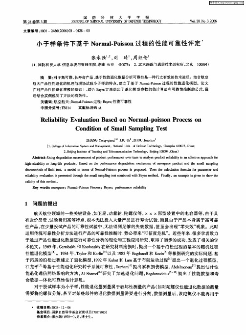
小子样条件下基于Normal-Poisson过程的性能可靠性评定

维普资讯
国防科技大学
堡
婴
：垫：型
文章编号：０一ｚ８（０６０ —０２一ｏ１１４６２ｏ）３１８５０
小子样条件下基于Ｎｒ１ｏｓｎ过程的性能可靠性评定ｏｍａＰｉｏ．ｓ
ｖｆｈｓｔｄｏｔｉｍｅｏ．ｈＫｅｒｓａｒｓａｅｙｗｏｄ：ｅｏｐｃ；Ｎｏｍａ— ｏｓｏｒｃｓ；ＢｙｓｅｏｍａｃｅｉｂｌｙｒｌＰｉｎＰｏｅｓａｅ；ｐｒｒｎｅｒａｉｔｓｆｌｉ
｝ｈｅａｉｙｏｎ－ｆｐｏｕｔａｄｏｅｐｒｒａｃｅｒａｏｅｈｎｓｆａｒｐｃｒｕｔｎｅｓａａｐｎｌ－ｌｂｉｒｌｇｌｅｒｃ．Ｂｓｎｔｆｍｎｅｄｇｄｔｎｍｃａｉｏｅｏａｅｐｄｃａｄｔｍｌｓｍｌｇｉｒｉｌｇｔｏｉｄｓｅｈｅｏａｉｍｓｏｈｌｉ
于通过产品性能退化数据进行可靠性分析的理论和工程应用研究，取得了初步的成功，发表了相关的学术论文。１６年，ｅｓａａＫｒｍｋ在研究材料磨损时，９９Ｇｒｂｌ和ｏｏｉｔｄｄｙ提出一个基于泊松过程的基本的随机过程性能退化模型－。１８年，ａｌ和Ｋｒｎｌ９４Ｔｙｒａｉ－以及１８年Ｂｇａｏ和Ｋｚ－等根据研究的实际问题，Ｊｏｌ２９５ｏｄｆｎｏｉ３ｎ基
航天产品性能退化的机理与现场试验小子样的特点，建立了基于ＮｍａＰｉｏ过程的性能退化模型。论文ｏａ－ｏｓｎｌｓ在对产品性能退化建模的基础上，结合Ｂｙｓａｅ方法给出了退化模型参数的估计算法和可靠性推断的公式，最后结合实例说明了方法的有效性。关键词：航空航天；ｏ￣．ｏｓ过程；ａｅ；ＮｍａＰｉｏ１ｓｎＢｙｓ性能可靠性

Zero-Truncated Poisson Lognormal分布函数包说明说明书

Package‘ztpln’October14,2022Type PackageTitle Zero-Truncated Poisson Lognormal DistributionVersion0.1.2Date2021-10-09Author Masatoshi KatabuchiMaintainer Masatoshi Katabuchi<********************>Description Functions for obtaining the density,random variatesand maximum likelihood estimates of the Zero-truncated Poisson lognormaldistribution and their mixture distribution.License MIT+ﬁle LICENSEURL https:///mattocci27/ztplnBugReports https:///mattocci27/ztpln/issuesDepends R(>=3.5)Imports DistributionUtils,Rcpp(>=0.12.0),mixtools,statsSuggests knitr,dplyr,ggplot2,rmarkdown,testthat,tidyr(>=1.0.0)LinkingTo Rcpp(>=0.12.0),RcppEigen(>=0.3.3.3.0),RcppNumerical(>=0.3-2)VignetteBuilder knitrEncoding UTF-8RoxygenNote7.1.2NeedsCompilation yesRepository CRANDate/Publication2021-10-0914:50:02UTCR topics documented:dztpln (2)dztplnm (3)ztplnMLE (4)ztplnmMLE (5)12dztplnIndex7 dztpln The zero-truncated compund poisson-lognormal distributionsDescriptionDensity function and random generation for Zero-Trauncated Poisson Lognormal distribution withparameters mu and sd sig.Usagedztpln(x,mu,sig,log=FALSE,type1=TRUE)rztpln(n,mu,sig,type1=TRUE)Argumentsx vector of(non-negative integer)quantiles.mu mean of lognormal distribution.sig standard deviation of lognormal distribution.log logical;if TRUE,probabilities p are given as log(p).type1logical;if TRUE,Use type1ztpln else use type2.n number of random values to return.DetailsA compound Poisson-lognormal distribution is a Poisson probability distribution where its param-eterλis a random variable with lognormal distribution,that is to say logλare normally distributedwith meanµand varianceσ2(Bulmer1974).The zero-truncated Poisson-lognormal distributioncan be derived from a zero-truncated Poisson distribution.Type1ZTPLN truncates zero based on Poisson-lognormal distribution and type2ZTPLN truncateszero based on zero-truncated Poisson distribution.For mathematical details,please see vignette("ztpln") Valuedztpln gives the(log)density and rztpln generates random variates.ReferencesBulmer,M.G.1974.On Fitting the Poisson Lognormal Distribution to Species-Abundance Data.Biometrics30:101-110.See Alsodztplnmdztplnm3Examplesrztpln(n=10,mu=0,sig=1,type1=TRUE)rztpln(n=10,mu=6,sig=4,type1=TRUE)dztpln(x=1:5,mu=1,sig=2)dztplnm The zero-truncated compund poisson-lognormal distributions mixtureDescriptionDensity function and random generation for Zero-Truncated Poisson Lognormal distribution withparameters mu,sig,and theta.Usagedztplnm(x,mu,sig,theta,log=FALSE,type1=TRUE)rztplnm(n,mu,sig,theta,type1=TRUE)Argumentsx vector of(non-negative integer)quantiles.mu vector of mean of lognormal distribution in sample.sig vector standard deviation of lognormal distribution in sample.theta vector of mixture weightslog logical;if TRUE,probabilities p are given as log(p).type1logical;if TRUE,Use type1ztpln else use type2.n number of random values to return.DetailsType1ZTPLN truncates zero based on Poisson-lognormal distribution and type2ZTPLN truncateszero based on zero-truncated Poisson distribution.For mathematical details,please see vignette("ztpln") Valuedztplnm gives the(log)density and rztplnm generates random variates.function,qpois gives thequantile function,and rpois generates random deviates.See AlsodztplnExamplesrztplnm(n=100,mu=c(0,5),sig=c(1,2),theta=c(0.2,0.8))dztplnm(x=1:100,mu=c(0,5),sig=c(1,2),theta=c(0.2,0.8))dztplnm(x=1:100,mu=c(0,5),sig=c(1,2),theta=c(0.2,0.8),type1=FALSE)ztplnMLE MLE for the Zero-truncated Poisson Lognormal distributionDescriptionztplnMLEﬁts the Zero-truncated Poisson lognormal distribution to data and estimates parameters mean mu and standard deviation sig in the lognormal distributionUsageztplnMLE(n,lower_mu=0,upper_mu=log(max(n)),lower_sig=0.001,upper_sig=10,type1=TRUE)Argumentsn a integer vector of countslower_mu,upper_munumeric values of lower and upper bounds for mean of the variables’s natruallogarithm.lower_sig,upper_signumeric values of lower and upper bounds for standard deviatoin of the vari-ables’s natrual logarithmtype1logical;if TRUE,Use type1ztpln else use type2.DetailsThe function searches the maximum likelihood estimates of mean mu and standard deviation sig using the optimization procedures in nlminb.Valueconvergence An integer code.0indicates successful convergence.iterations Number of iterations performed.message A character string giving any additional information returned by the optimizer, or NULL.For details,see PORT documentation.evaluation Number of objective function and gradient function evaluationsmu Maximum likelihood estimates of musig Maximum likelihood estimates of sigloglik loglikelihoodExamplesy<-rztpln(100,3,2)ztplnMLE(y)ztplnmMLE MLE for the Zero-truncated Poisson Lognormal mixture distribtuionDescriptionztplnmMLEﬁts the Zero-truncated Poisson lognormal mixture distribution to data and estimates pa-rameters mean mu,standard deviation sig and mixture weight theta in the lognormal distribution. UsageztplnmMLE(n,K=2,lower_mu=rep(0,K),upper_mu=rep(log(max(n)),K),lower_sig=rep(0.001,K),upper_sig=rep(10,K),lower_theta=rep(0.001,K),upper_theta=rep(0.999,K),type1=TRUE,message=FALSE)Argumentsn a vector of countsK number of componentslower_mu,upper_munumeric values of lower and upper bounds for mean of the variables’s naturallogarithm.lower_sig,upper_signumeric values of lower and upper bounds for standard deviation of the vari-ables’s natural logarithmlower_theta,upper_thetanumeric values of lower and upper bounds for mixture weights.type1logical;if TRUE,Use type1ztpln else use type2.message mean of lognormal distribution in sample3.DetailsThe function searches the maximum likelihood estimators of mean vector mu,standard deviation vector sig and mixture weight vector theta using the optimization procedures in nlminb.Valueconvergence An integer code.0indicates successful convergence.iterations Number of iterations performed.message A character string giving any additional information returned by the optimizer, or NULL.For details,see PORT documentation.evaluation Number of objective function and gradient function evaluationsmu Maximum likelihood estimates of musig Maximum likelihood estimates of sigtheta Maximum likelihood estimates of thetaloglik loglikelihoodExamplesy<-rztplnm(100,c(1,10),c(2,1),c(0.2,0.8))ztplnmMLE(y)Indexdztpln,2,3dztplnm,2,3nlminb,4,5rztpln(dztpln),2rztplnm(dztplnm),3ztplnMLE,4ztplnmMLE,57。

stata 指令(1)

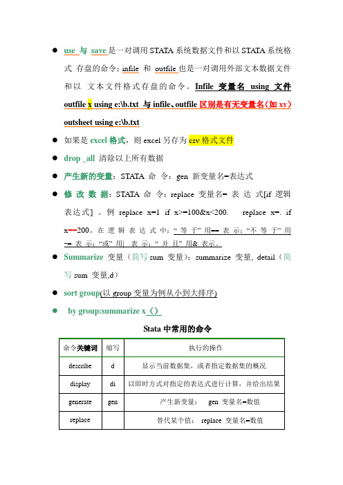
●use 与save是一对调用STATA系统数据文件和以STATA系统格式存盘的命令；infile 和outfile也是一对调用外部文本数据文件和以文本文件格式存盘的命令。

Infile 变量名using 文件outsheet using e:\b.txt●如果是excel格式，则excel另存为csv格式文件●drop _all清除以上所有数据●产生新的变量：STATA 命令：gen 新变量名=表达式●修改数据：STATA 命令：replace 变量名= 表达式[if 逻辑表达式] 。

例replace x=1 if x>=100&x<200. replace x=. if x==200。

在逻辑表达式中：“ 等于” 用== 表示；“不等于” 用~= 表示；“或” 用| 表示；“ 并且” 用& 表示。

●Summarize 变量（简写sum 变量）；summarize 变量, detail（简写sum 变量,d）●sort group(以group变量为例从小到大排序)●by group:summarize x（）Stata中常用的命令●(分组变量)tab1 变量名,g( 新变量名)。

该命令主要适用描述计数资料( 即：属性资料)。

●频数分布的常见错误：tab、tab1、tab2tab 1）用于生成单个变量的频数分布，其后只能跟一个变量；2）用于描述两个变量的交叉分布，其后只能接两个变量；所以tab后面最多接1个变量。

tab1 可以接多个变量，扥是只能分别生成各个变量的频数分布，不能生成交叉表。

tab2 可以生成多个双变量的交叉表。

●四分位数间距：上四分位数与下四分位数之差,用四分位数间距可反映变异程度的大小.1 Centile x【得中位数】。

centile x, c(25, 50, 75)【四分之一，中位数。

】{sum x, detail}也可以得到所需。

2 tabstat x[fw=f], st(q) {没expand f时，用此；有expand f, 则去掉fw=f}3expand xCentile x, c(25,50,75)●Tab x [fw=f]●频数分布表中要用到expand 变量名，后再计算个指标●graph x, bin(13) norm 【bin(13)表示频数图的组数为13。

统计学CH10 英文版

We saw earlier that point probabilities in continuous distributions were virtually zero. Likewise, we’d expect that the point estimator gets closer to the parameter value with an increased sample size, but point estimators don’t reflect the effects of larger sample sizes. Hence we will employ the interval estimator to estimate population parameters…
Copyright © 2009 Cengage Learning
Unbiased Estimators…
An unbiased estimator of a population parameter is an estimator whose expected value is equal to that parameter. E.g. the sample median is an unbiased estimator of the population mean µ since: E(Sample median) = µ
To do so we need the population parameters. Binomial: p Poisson: µ Normal: µ and σ Exponential: λ or µ
Cop we have been…
Copyright © 2009 Cengage Learning

概率论几种重要的分布

概率论几种重要的分布
概率论中有许多重要的分布，包括以下几种：
1. 正态分布（Normal Distribution）：也称为高斯分布，是最常见的分布之一。

它具有钟形曲线，对称，以及均值和方差完全定义。

在许多实际应用中，自然界中许多现象都遵循正态分布。

2. 二项分布（Binomial Distribution）：描述了在固定次数的独立重复试验中成功次数的概率分布。

每个试验有两个可能的结果，成功和失败，并且每次试验的成功概率保持不变。

3. 泊松分布（Poisson Distribution）：用于描述稀有事件在固定时间或空间上的发生次数的概率分布。

它假设事件发生的概率相等，且事件之间是相互独立的。

4. 均匀分布（Uniform Distribution）：也称为矩形分布，是一种概率分布，其中所有可能的结果的概率是相等的。

在定义了一个范围之后，均匀分布将这个范围内的概率均匀地分布。

5. 指数分布（Exponential Distribution）：用于描述独立事件发生间隔的概率分布。

它假设事件是以恒定速率独立地发生的，即它具有无记忆性。

6. t分布（Student t-Distribution）：用于小样本情况下的统计推断，当样本量较小时，t分布的尾部更加重，与正态分布相比，更容易出现极端值。

以上只是一些重要的分布，概率论还有很多其他的分布，根据实际应用的不同，可以选择合适的分布模型。

浅析概率论中常见的近似分布和其适用条件

浅析概率论中常见的近似分布和其适用条件内容摘要本文是一篇综述性质的文章，从随机变量序列的几种常见分布和它们之间的关系谈起，总结了应用泊松分布和正态分布来近似二项分布的发展过程、原理证明、适用条件和近似误差。

随后，通过一个具体计算的例子来说明这些近似定理的适用条件和如何在实际问题中灵活应用和辨别是否服从我们给出的定理条件。

最后，通过二项分布和超几何分布之间的联系，进一步阐述了用正态分布来近似超几何分布的判断方法和近似误差。

关键词：二项分布泊松分布正态分布超几何分布近似证明ABSTRACTBased on literature review, this essay starts with several common distributions of the random variable sequences and the relationships between them, and summarizes the development process, the demonstration of the principles, the applicable conditions and the approximate errors of using Normal distribution and Poisson distribution to approximate Binomial distribution .Then a specific example is presented to explain the application conditions of these theorems and how to use them flexibly in the practical problem to identify if the practical situation meets the conditions. Finally，the judgment method and approximate errors of using Normal distribution to approximate hypergeometric distribution are further expatiated by presenting the relationship between binomial distribution and hypergeometric distribution.KEY WORDS：binomial distribution Poisson distribution Normal distribution hypergeometric distribution poisson's theorem theorem’s demonstration 概率论与数理统计是一门研究随机现象统计规律性的一门数学学科，它起源于十七世纪中叶，在误差分析、人口统计、人寿保险等范畴中起到了十分重要的作用。

微积分基本公式

微积分公式sin x dx = -cos x + C cos x dx = sin x + C tan x dx = ln |sec x | + C cot x dx = ln |sin x | + Csec x dx = ln |sec x + tan x | + Ccsc x dx = ln |csc x – cot x | +Csin -1(-x) = -sin -1 x cos -1(-x) =- cos -1 xtan -1(-x) = -tan -1 x cot -1(-x) =- cot -1 x sec -1(-x) =- sec -1 xcsc -1(-x) = - csc -1 xsin -1 x dx = x sin -1x+21x -+C cos -1 x dx = x cos -1 x-21x -+Ctan -1 x dx = x tan -1 x-½ln (1+x 2)+C cot -1 x dx = x cot -1 x+½ln (1+x 2)+Csec -1 x dx = x sec -1 x- ln|x+12-x |+C csc -1 x dx = x csc -1x+ ln |x+12-x |+C tanh coth sinh x dx = cosh x + C cosh x dx = sinh x + C tanh x dx = ln | cosh x |+ C coth x dx = ln | sinh x | + Csech x dx = -2tan -1 (e -x ) + C csch x dx = 2 ln |xx e e 211---+| + C d uv = u d v + v d u d uv = uv = u d v + v d u →u d v = uv -v d ucos 2θ-sin 2θ=cos2θ cos 2θ+ sin 2θ=1cosh 2θ-sinh 2θ=1cosh 2θ+sinh 2θ=cosh2θsinh -1x dx = x sinh -1x-21x ++ Ccosh -1 x dx = x cosh -1 x-12-x + Ctanh -1 x dx = x tanh -1 x+ ½ ln |1-x 2|+ Ccoth -1 x dx = x coth -1 x- ½ ln |1-x 2|+ Csech -1x dx = x sech -1 x- sin -1x + Ccsch -1 x dx = x csch -1 x+ sinh -1 x + CabcαβγRsin x = x-!33x +!55x -!77x +…+)!12()1(12+-+n x n n + …cos x = 1-!22x +!44x -!66x +…+)!2()1(2n x n n -+ …ln (1+x) = x-22x +33x -44x +…+)!1()1(1+-+n x n n + …tan -1x = x-33x +55x -77x +…+)12()1(12+-+n x n n + …(1+x)r=1+r x+!2)1(-r r x 2+!3)2)(1(--r r r x 3+… -1<x<1 ∑=ni i 1= ½n (n +1)∑=ni i 12= 61 n (n +1)(2n +1) ∑=ni i 13= [½n (n +1)]2 Γ(x) = ⎰∞0t x-1e -t d t = 2⎰∞0t 2x-12t e -d t = ⎰∞0)1(ln tx-1 d tβ(m , n ) =⎰10x m -1(1-x)n -1d x =2⎰20sin π2m -1x cos 2n -1x d x= ⎰∞+-+01)1(nm m x x d x 希腊字母 (Greek Alphabets)大写小写读音大写小写读音大写小写读音 Α α alpha Ι ι iota Ρ ρrhoΒ β beta Κ κ kappa Σ σ, ς sigma Γ γ gamma Λ λ lambda Τ τ tau Δ δ delta Μ μ mu Υ υ upsilon Ε ε epsilon Ν ν nu Φ φ phi Ζ ζ zeta Ξ ξ xi Χ χ khi Η η eta Ο ο omicron Ψ ψ psi Θ θthetaΠπpiΩωomega倒数关系: sin θcsc θ=1; tan θcot θ=1; cos θsec θ=1 商数关系: tan θ=θθcos sin ; cot θ= θθsin cos 平方关系: cos 2θ+ sin 2θ=1; tan 2θ+ 1= sec 2θ; 1+ cot 2θ= csc 2θ順位低順位高;顺位高d 顺位低 ;0*=∞1 * = ∞∞= 0*01 = 0000 = )(0-∞e ; 0∞ = ∞⋅0e ; ∞1 = ∞⋅0e顺位一: 对数; 反三角(反双曲) 顺位二: 多项函数; 幂函数1 000 000 000 000 000 000 000 000 1024 yotta Y 1 000 000 000 000 000 000 000 1021 zetta Z1 000 000 000 000 000 000 1018 exa E1 000 000 000 000 000 1015 peta P1 000 000 000 000 1012 tera T 兆1 000 000 000 109 giga G 十亿1 000 000 106 mega M 百万1 000 103 kilo K 千100 102 hecto H 百10 101 deca D 十10-1 deci d 分，十分之一10-2 centi c 厘（或写作「厘」），百分之一10-3 milli m 毫，千分之一001 10-6 micro 微，百万分之一000 001 10-9 nano n 奈，十亿分之一000 000 001 10-12 pico p 皮，兆分之一000 000 000 001 10-15 femto f 飞（或作「费」），千兆分之一 000 000 000 000 001 10-18 atto a 阿000 000 000 000 000 001 10-21 zepto z000 000 000 000 000 000 001 10-24 yocto y。

拟合优度检验和独立性检验英文版

© 2011 Cengage Learning. All Rights Reserved. May not be scanned, copied or duplicated, or posted to a publicly accessible website, in whole or in part.
Slide 9
Multinomial Distribution Goodness of Fit Test
Rejection Rule Reject H0 if p-value < .05 or χ2 > 7.815. With α = .05 and k-1=4-1=3 degrees of freedom
Slide 5
Hypothesis (Goodness of Fit) Test for Proportions of a Multinomial Population
5. Rejection rule: p-value approach: Reject H0 if p-value < α Reject H0 if
Slide 8
Multinomial Distribution Goodness of Fit Test
Hypotheses H0: pC = pL = pS = pA = .25 Ha: The population proportions are not pC = .25, pL = .25, pS = .25, and pA = .25 where: pC = population proportion that purchase a colonial pL = population proportion that purchase a log cabin pS = population proportion that purchase a split-level splitpA = population proportion that purchase an A-frame A-

1、下载文档前请自行甄别文档内容的完整性，平台不提供额外的编辑、内容补充、找答案等附加服务。
2、"仅部分预览"的文档,不可在线预览部分如存在完整性等问题,可反馈申请退款(可完整预览的文档不适用该条件!)。
3、如文档侵犯您的权益，请联系客服反馈,我们会尽快为您处理(人工客服工作时间：9:00-18:30)。

二项分布和Poisson分布均是常见的离散型分布，在分类资料的统计推断中有非常广泛的应用。

一、二项分布的概念及应用条件
1. 二项分布的概念:
如某实验中小白鼠染毒后死亡概率P为0.8,则生存概率为=1-P=0.2，故
对一只小白鼠进行实验的结果为：死（概率为P）或生（概率为1-P）
对二只小白鼠（甲乙）进行实验的结果为：甲乙均死（概率为P^2）、甲死乙生[概率为P(1-P)]、乙死甲生[概率为(1-P）P]或甲乙均生[概率为(1-P^2]，概率相加得P2+P(1-P)+(1-P）P+(1-P）2=[P+(1-P)]2
依此类推，对n只小白鼠进行实验，所有可能结果的概率相加得
P^n+1C n1P(1-P)^(n-1)+...+C n x P^x(1-P)^(n-x)+...+(1-P)^x=[P+(1-P)]^n 其中n为样本含量,即事件发生总数，x为某事件出现次数, C n x P^x(1-P)^(n-x)为二项式通式，C n x =n!/x!(n-x)!, P为总体率。

因此，二项分布是说明结果只有两种情况的n次实验中发生某种结果为x次的概率分布。

其概率密度为：
P(x)= C n x Px(1-P)n-x, x=0,1,...n。

2. 二项分布的应用条件:
医学领域有许多二分类记数资料都符合二项分布(传染病和遗传病除外)，但应用时仍应注意考察是否满足以下应用条件：(1) 每次实验只有两类对立的结果；(2) n次事件相互独立；(3) 每次实验某类结果的发生的概率是一个常数。

3. 二项分布的累计概率
二项分布下最多发生k例阳性的概率为发生0例阳性、1例阳性、...、直至k 例阳性的概率之和。

至少发生k例阳性的概率为发生k例阳性、k+1例阳性、...、直至n例阳性的概率之和。

4. 二项分布的图形
二项分布的图形有如下特征：(1)二项分布图形的形状取决于P 和n 的大小；(2) 当P=0.5时，无论n的大小，均为对称分布；(3) 当P<或>0.5 ,n较小时为偏态分布,n较大时逼近正态分布。

5. 二项分布的均数和标准差
二项分布的均数µ=np，当用率表示时µ=p
二项分布的标准差为np(1-p)的算术平方根，当用率表示时为p(1-p)的算术平方根。

二、二项分布的应用
二项分布主要用于符合二项分布分类资料的率的区间估计和假设检验。

当P=0.5或n较大，nP及n(1-P)均大于等于5时，可用(p-u0.05sp,p+u0.05sp)对总体率进行95%的区间估计。

当总体率P接近0.5，阳性数x较小时，可直接计算二项分布的累计概率进行单侧的假设检验。

当P=0.5或n较大，nP及n(1-P)均大于等于5时，可用正态近似法进行样本率与总体率，两个样本率比较的u检验。

三、Poisson分布的概念及应用条件
1. Poisson分布的概念:
Poisson分布是二项分布n很大而P很小时的特殊形式，是两分类资料在n次实
验中发生x次某种结果的概率分布。

其概率密度函数为：P(x)=μx
x!
e−μ
x=0,1,2...n，其中e为自然对数的底，µ为总体均数，x为事件发生的阳性数。

2. Poisson分布的应用条件:
医学领域中有很多稀有疾病(如肿瘤,交通事故等）资料都符合Poisson分布，但应用中仍应注意要满足以下条件：（1) 两类结果要相互对立；（2) n次试验相互独立；（3) n应很大, P应很小。

3. Poisson分布的概率
Poisson分布的概率利用以下递推公式很容易求得：
P(0)=e−μ
P(x+1)=P(x)*µ/x+1, x=0,1,2,...
4. Poisson分布的性质:
(1) Poisson分布均数与方差相等；
(2) Poisson分布均数µ较小时呈偏态,µ>=20时近似正态；
(3) n很大, P很小，nP=µ为常数时二项分布趋近于Poisson分布；
(4) n个独立的Poisson分布相加仍符合Poisson分布
四、Poisson分布的应用
Poisson分布也主要用于符合Poisson分布分类资料率的区间估计和假设检验。

当µ>=20时，根据正态近似的原理，可用（x-u0.05*x的算术平方根，x+u0.05*x 的算术平方根）对总体均数进行95%的区间估计。

同样，也可通过直接计算Poisson分布的累计概率进行单侧的假设检验，在符合正态近似条件时，也可用u检验进行样本率与总体率，两个样本率比较的假设检验。