Critical Edges in Perfect Graphs and Some Polyhedral Consequences
学数学的必看GTM经典著作下载三
学数学的必看GTM经典著作下载三202 Introduction to Topological Manifolds,John M.Lee(拓扑流形入门)镜像下载(4874KB,英文版,DJVU格式,支持关键词检索,点击打开下载页面,支持迅雷、快车下载)203 The Symmetric Group,Bruce E.Sagan 204 Galois Theory,Jean-Pierre Escofier 205 Rational Homotopy Theory,Yves Félix,Stephen Halperin,Jean-Claude Thomas(有理同伦论)镜像下载(5220KB,英文版,DJVU格式,支持关键词检索,点击打开下载页面,支持迅雷、快车下载)有理同伦论是由Sullivan创立的。
Felix是新鲁汶大学(法语鲁汶大学)的教授,第二作者是著名的华人逻辑学家王浩的学生。
206 Problems in Analytic Number Theory,M.Ram Murty 207 Algebraic Graph Theory,Godsil,Royle(代数图论)镜像下载(4062KB,英文版,DJVU格式,支持关键词检索,点击打开下载页面,支持迅雷、快车下载)Godsil是加拿大滑铁卢大学的教授,代数组合图论的权威。
曾任JAC的主编,现在是组合学期刊(JC)电子版的主编。
Royle是UWA的副教授。
208 Analysis for Applied Mathematics,Ward Cheney 209 AShort Course on Spectral Theory,William Arveson(谱理论简明教程)镜像下载(4366KB,英文版,DJVU格式,支持关键词检索,点击打开下载页面,支持迅雷、快车下载)本书给读者提供谱论-被称之为解决算子理论基本问题的基本工具,并主要计算了无限维空间特别是希尔伯特空间算子的谱。
图论及其应用

图和子图 图和简单图图 G = (V, E), 其中 V = {νv v v ,......,,21} V ---顶点集, ν---顶点数E = {e e e 12,,......,ε}E ---边集, ε---边数例。
左图中, V={a, b,......,f}, E={p,q, ae, af,......,ce, cf} 注意, 左图仅仅是图G 的几何实现(代表), 它们有无穷多个。
真正的 图G 是上面所给出式子,它与顶点的位置、边的形状等无关。
不过今后对两者将经常不加以区别。
称 边 ad 与顶点 a (及d) 相关联。
也称 顶点 b(及 f) 与边 bf 相关联。
称顶点a 与e 相邻。
称有公共端点的一些边彼此相邻,例如p 与af 。
环(loop ,selfloop ):如边 l 。
棱(link ):如边ae 。
重边:如边p 及边q 。
简单图:(simple graph )无环,无重边 平凡图:仅有一个顶点的图(可有多条环)。
一条边的端点:它的两个顶点。
记号:νε()(),()().G V G G E G ==。
习题1.1.1 若G 为简单图,则εν≤⎛⎝ ⎫⎭⎪2 。
1.1.2 n ( ≥ 4 )个人中,若每4人中一定有一人认识其他3人,则一定有一 人认识其他n-1人。
同构在下图中, 图G 恒等于图H , 记为 G = H ⇔ V (G)=V(H), E(G)=E(H)。
图G 同构于图F ⇔ V(G)与V(F), E(G)与E(F)之间各存在一一对应关系,且这二对应关系保持关联关系。
记为 G ≅F 。
注 往往将同构慨念引伸到非标号图中,以表达两个图在结构上是否相同。
de f G = (V, E)y z w cG =(V , E )w cyz H =(V ’, E ’)’a ’c ’y ’e ’z ’F =(V ’’, E ’’)注 判定两个图是否同构是NP-hard 问题。
完全图(complete graph) Kn空图(empty g.) ⇔ E = ∅ 。
Kernels and regularization on graphs

Kernels and Regularization on GraphsAlexander J.Smola1and Risi Kondor21Machine Learning Group,RSISEAustralian National UniversityCanberra,ACT0200,AustraliaAlex.Smola@.au2Department of Computer ScienceColumbia University1214Amsterdam Avenue,M.C.0401New York,NY10027,USArisi@Abstract.We introduce a family of kernels on graphs based on thenotion of regularization operators.This generalizes in a natural way thenotion of regularization and Greens functions,as commonly used forreal valued functions,to graphs.It turns out that diffusion kernels canbe found as a special case of our reasoning.We show that the class ofpositive,monotonically decreasing functions on the unit interval leads tokernels and corresponding regularization operators.1IntroductionThere has recently been a surge of interest in learning algorithms that operate on input spaces X other than R n,specifically,discrete input spaces,such as strings, graphs,trees,automata etc..Since kernel-based algorithms,such as Support Vector Machines,Gaussian Processes,Kernel PCA,etc.capture the structure of X via the kernel K:X×X→R,as long as we can define an appropriate kernel on our discrete input space,these algorithms can be imported wholesale, together with their error analysis,theoretical guarantees and empirical success.One of the most general representations of discrete metric spaces are graphs. Even if all we know about our input space are local pairwise similarities between points x i,x j∈X,distances(e.g shortest path length)on the graph induced by these similarities can give a useful,more global,sense of similarity between objects.In their work on Diffusion Kernels,Kondor and Lafferty[2002]gave a specific construction for a kernel capturing this structure.Belkin and Niyogi [2002]proposed an essentially equivalent construction in the context of approx-imating data lying on surfaces in a high dimensional embedding space,and in the context of leveraging information from unlabeled data.In this paper we put these earlier results into the more principled framework of Regularization Theory.We propose a family of regularization operators(equiv-alently,kernels)on graphs that include Diffusion Kernels as a special case,and show that this family encompasses all possible regularization operators invariant under permutations of the vertices in a particular sense.2Alexander Smola and Risi KondorOutline of the Paper:Section2introduces the concept of the graph Laplacian and relates it to the Laplace operator on real valued functions.Next we define an extended class of regularization operators and show why they have to be es-sentially a function of the Laplacian.An analogy to real valued Greens functions is established in Section3.3,and efficient methods for computing such functions are presented in Section4.We conclude with a discussion.2Laplace OperatorsAn undirected unweighted graph G consists of a set of vertices V numbered1to n,and a set of edges E(i.e.,pairs(i,j)where i,j∈V and(i,j)∈E⇔(j,i)∈E). We will sometimes write i∼j to denote that i and j are neighbors,i.e.(i,j)∈E. The adjacency matrix of G is an n×n real matrix W,with W ij=1if i∼j,and 0otherwise(by construction,W is symmetric and its diagonal entries are zero). These definitions and most of the following theory can trivially be extended toweighted graphs by allowing W ij∈[0,∞).Let D be an n×n diagonal matrix with D ii=jW ij.The Laplacian of Gis defined as L:=D−W and the Normalized Laplacian is˜L:=D−12LD−12= I−D−12W D−12.The following two theorems are well known results from spectral graph theory[Chung-Graham,1997]:Theorem1(Spectrum of˜L).˜L is a symmetric,positive semidefinite matrix, and its eigenvaluesλ1,λ2,...,λn satisfy0≤λi≤2.Furthermore,the number of eigenvalues equal to zero equals to the number of disjoint components in G.The bound on the spectrum follows directly from Gerschgorin’s Theorem.Theorem2(L and˜L for Regular Graphs).Now let G be a regular graph of degree d,that is,a graph in which every vertex has exactly d neighbors.ThenL=d I−W and˜L=I−1d W=1dL.Finally,W,L,˜L share the same eigenvectors{v i},where v i=λ−1iW v i=(d−λi)−1L v i=(1−d−1λi)−1˜L v i for all i.L and˜L can be regarded as linear operators on functions f:V→R,or,equiv-alently,on vectors f=(f1,f2,...,f n) .We could equally well have defined Lbyf,L f =f L f=−12i∼j(f i−f j)2for all f∈R n,(1)which readily generalizes to graphs with a countably infinite number of vertices.The Laplacian derives its name from its analogy with the familiar Laplacianoperator∆=∂2∂x21+∂2∂x22+...+∂2∂x2mon continuous spaces.Regarding(1)asinducing a semi-norm f L= f,L f on R n,the analogous expression for∆defined on a compact spaceΩisf ∆= f,∆f =Ωf(∆f)dω=Ω(∇f)·(∇f)dω.(2)Both(1)and(2)quantify how much f and f vary locally,or how“smooth”they are over their respective domains.Kernels and Regularization on Graphs3 More explicitly,whenΩ=R m,up to a constant,−L is exactly thefinite difference discretization of∆on a regular lattice:∆f(x)=mi=1∂2∂x2if≈mi=1∂∂x if(x+12e i)−∂∂x if(x−12e i)δ≈mi=1f(x+e i)+f(x−e i)−2f(x)δ2=1δ2mi=1(f x1,...,x i+1,...,x m+f x1,...,x i−1,...,x m−2f x1,...,x m)=−1δ2[L f]x1,...,x m,where e1,e2,...,e m is an orthogonal basis for R m normalized to e i =δ, the vertices of the lattice are at x=x1e1+...+x m e m with integer valuedcoordinates x i∈N,and f x1,x2,...,x m=f(x).Moreover,both the continuous and the dis-crete Laplacians are canonical operators on their respective domains,in the sense that they are invariant under certain natural transformations of the underlying space,and in this they are essentially unique.Regular grid in two dimensionsThe Laplace operator∆is the unique self-adjoint linear second order differ-ential operator invariant under transformations of the coordinate system under the action of the special orthogonal group SO m,i.e.invariant under rotations. This well known result can be seen by using Schur’s lemma and the fact that SO m is irreducible on R m.We now show a similar result for L.Here the permutation group plays a similar role to SO m.We need some additional definitions:denote by S n the group of permutations on{1,2,...,n}withπ∈S n being a specific permutation taking i∈{1,2,...n}toπ(i).The so-called defining representation of S n consists of n×n matricesΠπ,such that[Ππ]i,π(i)=1and all other entries ofΠπare zero. Theorem3(Permutation Invariant Linear Functions on Graphs).Let L be an n×n symmetric real matrix,linearly related to the n×n adjacency matrix W,i.e.L=T[W]for some linear operator L in a way invariant to permutations of vertices in the sense thatΠ πT[W]Ππ=TΠ πWΠπ(3)for anyπ∈S n.Then L is related to W by a linear combination of the follow-ing three operations:identity;row/column sums;overall sum;row/column sum restricted to the diagonal of L;overall sum restricted to the diagonal of W. Proof LetL i1i2=T[W]i1i2:=ni3=1ni4=1T i1i2i3i4W i3i4(4)with T∈R n4.Eq.(3)then implies Tπ(i1)π(i2)π(i3)π(i4)=T i1i2i3i4for anyπ∈S n.4Alexander Smola and Risi KondorThe indices of T can be partitioned by the equality relation on their values,e.g.(2,5,2,7)is of the partition type [13|2|4],since i 1=i 3,but i 2=i 1,i 4=i 1and i 2=i 4.The key observation is that under the action of the permutation group,elements of T with a given index partition structure are taken to elements with the same index partition structure,e.g.if i 1=i 3then π(i 1)=π(i 3)and if i 1=i 3,then π(i 1)=π(i 3).Furthermore,an element with a given index index partition structure can be mapped to any other element of T with the same index partition structure by a suitable choice of π.Hence,a necessary and sufficient condition for (4)is that all elements of T of a given index partition structure be equal.Therefore,T must be a linear combination of the following tensors (i.e.multilinear forms):A i 1i 2i 3i 4=1B [1,2]i 1i 2i 3i 4=δi 1i 2B [1,3]i 1i 2i 3i 4=δi 1i 3B [1,4]i 1i 2i 3i 4=δi 1i 4B [2,3]i 1i 2i 3i 4=δi 2i 3B [2,4]i 1i 2i 3i 4=δi 2i 4B [3,4]i 1i 2i 3i 4=δi 3i 4C [1,2,3]i 1i 2i 3i 4=δi 1i 2δi 2i 3C [2,3,4]i 1i 2i 3i 4=δi 2i 3δi 3i 4C [3,4,1]i 1i 2i 3i 4=δi 3i 4δi 4i 1C [4,1,2]i 1i 2i 3i 4=δi 4i 1δi 1i 2D [1,2][3,4]i 1i 2i 3i 4=δi 1i 2δi 3i 4D [1,3][2,4]i 1i 2i 3i 4=δi 1i 3δi 2i 4D [1,4][2,3]i 1i 2i 3i 4=δi 1i 4δi 2i 3E [1,2,3,4]i 1i 2i 3i 4=δi 1i 2δi 1i 3δi 1i 4.The tensor A puts the overall sum in each element of L ,while B [1,2]returns the the same restricted to the diagonal of L .Since W has vanishing diagonal,B [3,4],C [2,3,4],C [3,4,1],D [1,2][3,4]and E [1,2,3,4]produce zero.Without loss of generality we can therefore ignore them.By symmetry of W ,the pairs (B [1,3],B [1,4]),(B [2,3],B [2,4]),(C [1,2,3],C [4,1,2])have the same effect on W ,hence we can set the coefficient of the second member of each to zero.Furthermore,to enforce symmetry on L ,the coefficient of B [1,3]and B [2,3]must be the same (without loss of generality 1)and this will give the row/column sum matrix ( k W ik )+( k W kl ).Similarly,C [1,2,3]and C [4,1,2]must have the same coefficient and this will give the row/column sum restricted to the diagonal:δij [( k W ik )+( k W kl )].Finally,by symmetry of W ,D [1,3][2,4]and D [1,4][2,3]are both equivalent to the identity map.The various row/column sum and overall sum operations are uninteresting from a graph theory point of view,since they do not heed to the topology of the graph.Imposing the conditions that each row and column in L must sum to zero,we recover the graph Laplacian.Hence,up to a constant factor and trivial additive components,the graph Laplacian (or the normalized graph Laplacian if we wish to rescale by the number of edges per vertex)is the only “invariant”differential operator for given W (or its normalized counterpart ˜W ).Unless stated otherwise,all results below hold for both L and ˜L (albeit with a different spectrum)and we will,in the following,focus on ˜Ldue to the fact that its spectrum is contained in [0,2].Kernels and Regularization on Graphs5 3RegularizationThe fact that L induces a semi-norm on f which penalizes the changes between adjacent vertices,as described in(1),indicates that it may serve as a tool to design regularization operators.3.1Regularization via the Laplace OperatorWe begin with a brief overview of translation invariant regularization operators on continuous spaces and show how they can be interpreted as powers of∆.This will allow us to repeat the development almost verbatim with˜L(or L)instead.Some of the most successful regularization functionals on R n,leading to kernels such as the Gaussian RBF,can be written as[Smola et al.,1998]f,P f :=|˜f(ω)|2r( ω 2)dω= f,r(∆)f .(5)Here f∈L2(R n),˜f(ω)denotes the Fourier transform of f,r( ω 2)is a function penalizing frequency components|˜f(ω)|of f,typically increasing in ω 2,and finally,r(∆)is the extension of r to operators simply by applying r to the spectrum of∆[Dunford and Schwartz,1958]f,r(∆)f =if,ψi r(λi) ψi,fwhere{(ψi,λi)}is the eigensystem of∆.The last equality in(5)holds because applications of∆become multiplications by ω 2in Fourier space.Kernels are obtained by solving the self-consistency condition[Smola et al.,1998]k(x,·),P k(x ,·) =k(x,x ).(6) One can show that k(x,x )=κ(x−x ),whereκis equal to the inverse Fourier transform of r−1( ω 2).Several r functions have been known to yield good results.The two most popular are given below:r( ω 2)k(x,x )r(∆)Gaussian RBF expσ22ω 2exp−12σ2x−x 2∞i=0σ2ii!∆iLaplacian RBF1+σ2 ω 2exp−1σx−x1+σ2∆In summary,regularization according to(5)is carried out by penalizing˜f(ω) by a function of the Laplace operator.For many results in regularization theory one requires r( ω 2)→∞for ω 2→∞.3.2Regularization via the Graph LaplacianIn complete analogy to(5),we define a class of regularization functionals on graphs asf,P f := f,r(˜L)f .(7)6Alexander Smola and Risi KondorFig.1.Regularization function r (λ).From left to right:regularized Laplacian (σ2=1),diffusion process (σ2=1),one-step random walk (a =2),4-step random walk (a =2),inverse cosine.Here r (˜L )is understood as applying the scalar valued function r (λ)to the eigen-values of ˜L ,that is,r (˜L ):=m i =1r (λi )v i v i ,(8)where {(λi ,v i )}constitute the eigensystem of ˜L .The normalized graph Lapla-cian ˜Lis preferable to L ,since ˜L ’s spectrum is contained in [0,2].The obvious goal is to gain insight into what functions are appropriate choices for r .–From (1)we infer that v i with large λi correspond to rather uneven functions on the graph G .Consequently,they should be penalized more strongly than v i with small λi .Hence r (λ)should be monotonically increasing in λ.–Requiring that r (˜L) 0imposes the constraint r (λ)≥0for all λ∈[0,2].–Finally,we can limit ourselves to r (λ)expressible as power series,since the latter are dense in the space of C 0functions on bounded domains.In Section 3.5we will present additional motivation for the choice of r (λ)in the context of spectral graph theory and segmentation.As we shall see,the following functions are of particular interest:r (λ)=1+σ2λ(Regularized Laplacian)(9)r (λ)=exp σ2/2λ(Diffusion Process)(10)r (λ)=(aI −λ)−1with a ≥2(One-Step Random Walk)(11)r (λ)=(aI −λ)−p with a ≥2(p -Step Random Walk)(12)r (λ)=(cos λπ/4)−1(Inverse Cosine)(13)Figure 1shows the regularization behavior for the functions (9)-(13).3.3KernelsThe introduction of a regularization matrix P =r (˜L)allows us to define a Hilbert space H on R m via f,f H := f ,P f .We now show that H is a reproducing kernel Hilbert space.Kernels and Regularization on Graphs 7Theorem 4.Denote by P ∈R m ×m a (positive semidefinite)regularization ma-trix and denote by H the image of R m under P .Then H with dot product f,f H := f ,P f is a Reproducing Kernel Hilbert Space and its kernel is k (i,j )= P −1ij ,where P −1denotes the pseudo-inverse if P is not invertible.Proof Since P is a positive semidefinite matrix,we clearly have a Hilbert space on P R m .To show the reproducing property we need to prove thatf (i )= f,k (i,·) H .(14)Note that k (i,j )can take on at most m 2different values (since i,j ∈[1:m ]).In matrix notation (14)means that for all f ∈Hf (i )=f P K i,:for all i ⇐⇒f =f P K.(15)The latter holds if K =P −1and f ∈P R m ,which proves the claim.In other words,K is the Greens function of P ,just as in the continuous case.The notion of Greens functions on graphs was only recently introduced by Chung-Graham and Yau [2000]for L .The above theorem extended this idea to arbitrary regularization operators ˆr (˜L).Corollary 1.Denote by P =r (˜L )a regularization matrix,then the correspond-ing kernel is given by K =r −1(˜L ),where we take the pseudo-inverse wherever necessary.More specifically,if {(v i ,λi )}constitute the eigensystem of ˜L,we have K =mi =1r −1(λi )v i v i where we define 0−1≡0.(16)3.4Examples of KernelsBy virtue of Corollary 1we only need to take (9)-(13)and plug the definition of r (λ)into (16)to obtain formulae for computing K .This yields the following kernel matrices:K =(I +σ2˜L)−1(Regularized Laplacian)(17)K =exp(−σ2/2˜L)(Diffusion Process)(18)K =(aI −˜L)p with a ≥2(p -Step Random Walk)(19)K =cos ˜Lπ/4(Inverse Cosine)(20)Equation (18)corresponds to the diffusion kernel proposed by Kondor and Laf-ferty [2002],for which K (x,x )can be visualized as the quantity of some sub-stance that would accumulate at vertex x after a given amount of time if we injected the substance at vertex x and let it diffuse through the graph along the edges.Note that this involves matrix exponentiation defined via the limit K =exp(B )=lim n →∞(I +B/n )n as opposed to component-wise exponentiation K i,j =exp(B i,j ).8Alexander Smola and Risi KondorFig.2.Thefirst8eigenvectors of the normalized graph Laplacian corresponding to the graph drawn above.Each line attached to a vertex is proportional to the value of the corresponding eigenvector at the vertex.Positive values(red)point up and negative values(blue)point down.Note that the assignment of values becomes less and less uniform with increasing eigenvalue(i.e.from left to right).For(17)it is typically more efficient to deal with the inverse of K,as it avoids the costly inversion of the sparse matrix˜L.Such situations arise,e.g.,in Gaussian Process estimation,where K is the covariance matrix of a stochastic process[Williams,1999].Regarding(19),recall that(aI−˜L)p=((a−1)I+˜W)p is up to scaling terms equiv-alent to a p-step random walk on the graphwith random restarts(see Section A for de-tails).In this sense it is similar to the dif-fusion kernel.However,the fact that K in-volves only afinite number of products ofmatrices makes it much more attractive forpractical purposes.In particular,entries inK ij can be computed cheaply using the factthat˜L is a sparse matrix.A nearest neighbor graph.Finally,the inverse cosine kernel treats lower complexity functions almost equally,with a significant reduction in the upper end of the spectrum.Figure2 shows the leading eigenvectors of the graph drawn above and Figure3provide examples of some of the kernels discussed above.3.5Clustering and Spectral Graph TheoryWe could also have derived r(˜L)directly from spectral graph theory:the eigen-vectors of the graph Laplacian correspond to functions partitioning the graph into clusters,see e.g.,[Chung-Graham,1997,Shi and Malik,1997]and the ref-erences therein.In general,small eigenvalues have associated eigenvectors which vary little between adjacent vertices.Finding the smallest eigenvectors of˜L can be seen as a real-valued relaxation of the min-cut problem.3For instance,the smallest eigenvalue of˜L is0,its corresponding eigenvector is D121n with1n:=(1,...,1)∈R n.The second smallest eigenvalue/eigenvector pair,also often referred to as the Fiedler-vector,can be used to split the graph 3Only recently,algorithms based on the celebrated semidefinite relaxation of the min-cut problem by Goemans and Williamson[1995]have seen wider use[Torr,2003]in segmentation and clustering by use of spectral bundle methods.Kernels and Regularization on Graphs9Fig.3.Top:regularized graph Laplacian;Middle:diffusion kernel with σ=5,Bottom:4-step random walk kernel.Each figure displays K ij for fixed i .The value K ij at vertex i is denoted by a bold line.Note that only adjacent vertices to i bear significant value.into two distinct parts [Weiss,1999,Shi and Malik,1997],and further eigenvec-tors with larger eigenvalues have been used for more finely-grained partitions of the graph.See Figure 2for an example.Such a decomposition into functions of increasing complexity has very de-sirable properties:if we want to perform estimation on the graph,we will wish to bias the estimate towards functions which vary little over large homogeneous portions 4.Consequently,we have the following interpretation of f,f H .As-sume that f = i βi v i ,where {(v i ,λi )}is the eigensystem of ˜L.Then we can rewrite f,f H to yield f ,r (˜L )f = i βi v i , j r (λj )v j v j l βl v l = iβ2i r (λi ).(21)This means that the components of f which vary a lot over coherent clusters in the graph are penalized more strongly,whereas the portions of f ,which are essentially constant over clusters,are preferred.This is exactly what we want.3.6Approximate ComputationOften it is not necessary to know all values of the kernel (e.g.,if we only observe instances from a subset of all positions on the graph).There it would be wasteful to compute the full matrix r (L )−1explicitly,since such operations typically scale with O (n 3).Furthermore,for large n it is not desirable to compute K via (16),that is,by computing the eigensystem of ˜Land assembling K directly.4If we cannot assume a connection between the structure of the graph and the values of the function to be estimated on it,the entire concept of designing kernels on graphs obviously becomes meaningless.10Alexander Smola and Risi KondorInstead,we would like to take advantage of the fact that ˜L is sparse,and con-sequently any operation ˜Lαhas cost at most linear in the number of nonzero ele-ments of ˜L ,hence the cost is bounded by O (|E |+n ).Moreover,if d is the largest degree of the graph,then computing L p e i costs at most |E | p −1i =1(min(d +1,n ))ioperations:at each step the number of non-zeros in the rhs decreases by at most a factor of d +1.This means that as long as we can approximate K =r −1(˜L )by a low order polynomial,say ρ(˜L ):= N i =0βi ˜L i ,significant savings are possible.Note that we need not necessarily require a uniformly good approximation and put the main emphasis on the approximation for small λ.However,we need to ensure that ρ(˜L)is positive semidefinite.Diffusion Kernel:The fact that the series r −1(x )=exp(−βx )= ∞m =0(−β)m x m m !has alternating signs shows that the approximation error at r −1(x )is boundedby (2β)N +1(N +1)!,if we use N terms in the expansion (from Theorem 1we know that ˜L≤2).For instance,for β=1,10terms are sufficient to obtain an error of the order of 10−4.Variational Approximation:In general,if we want to approximate r −1(λ)on[0,2],we need to solve the L ∞([0,2])approximation problemminimize β, subject to N i =0βi λi −r −1(λ) ≤ ∀λ∈[0,2](22)Clearly,(22)is equivalent to minimizing sup ˜L ρ(˜L )−r−1(˜L ) ,since the matrix norm is determined by the largest eigenvalues,and we can find ˜Lsuch that the discrepancy between ρ(λ)and r −1(λ)is attained.Variational problems of this form have been studied in the literature,and their solution may provide much better approximations to r −1(λ)than a truncated power series expansion.4Products of GraphsAs we have already pointed out,it is very expensive to compute K for arbitrary ˆr and ˜L.For special types of graphs and regularization,however,significant computational savings can be made.4.1Factor GraphsThe work of this section is a direct extension of results by Ellis [2002]and Chung-Graham and Yau [2000],who study factor graphs to compute inverses of the graph Laplacian.Definition 1(Factor Graphs).Denote by (V,E )and (V ,E )the vertices V and edges E of two graphs,then the factor graph (V f ,E f ):=(V,E )⊗(V ,E )is defined as the graph where (i,i )∈V f if i ∈V and i ∈V ;and ((i,i ),(j,j ))∈E f if and only if either (i,j )∈E and i =j or (i ,j )∈E and i =j .Kernels and Regularization on Graphs 11For instance,the factor graph of two rings is a torus.The nice property of factor graphs is that we can compute the eigenvalues of the Laplacian on products very easily (see e.g.,Chung-Graham and Yau [2000]):Theorem 5(Eigenvalues of Factor Graphs).The eigenvalues and eigen-vectors of the normalized Laplacian for the factor graph between a regular graph of degree d with eigenvalues {λj }and a regular graph of degree d with eigenvalues {λ l }are of the form:λfact j,l =d d +d λj +d d +d λ l(23)and the eigenvectors satisfy e j,l(i,i )=e j i e l i ,where e j is an eigenvector of ˜L and e l is an eigenvector of ˜L.This allows us to apply Corollary 1to obtain an expansion of K asK =(r (L ))−1=j,l r −1(λjl )e j,l e j,l .(24)While providing an explicit recipe for the computation of K ij without the need to compute the full matrix K ,this still requires O (n 2)operations per entry,which may be more costly than what we want (here n is the number of vertices of the factor graph).Two methods for computing (24)become evident at this point:if r has a special structure,we may exploit this to decompose K into the products and sums of terms depending on one of the two graphs alone and pre-compute these expressions beforehand.Secondly,if one of the two terms in the expansion can be computed for a rather general class of values of r (x ),we can pre-compute this expansion and only carry out the remainder corresponding to (24)explicitly.4.2Product Decomposition of r (x )Central to our reasoning is the observation that for certain r (x ),the term 1r (a +b )can be expressed in terms of a product and sum of terms depending on a and b only.We assume that 1r (a +b )=M m =1ρn (a )˜ρn (b ).(25)In the following we will show that in such situations the kernels on factor graphs can be computed as an analogous combination of products and sums of kernel functions on the terms constituting the ingredients of the factor graph.Before we do so,we briefly check that many r (x )indeed satisfy this property.exp(−β(a +b ))=exp(−βa )exp(−βb )(26)(A −(a +b ))= A 2−a + A 2−b (27)(A −(a +b ))p =p n =0p n A 2−a n A 2−b p −n (28)cos (a +b )π4=cos aπ4cos bπ4−sin aπ4sin bπ4(29)12Alexander Smola and Risi KondorIn a nutshell,we will exploit the fact that for products of graphs the eigenvalues of the joint graph Laplacian can be written as the sum of the eigenvalues of the Laplacians of the constituent graphs.This way we can perform computations on ρn and˜ρn separately without the need to take the other part of the the product of graphs into account.Definek m(i,j):=l ρldλld+de l i e l j and˜k m(i ,j ):=l˜ρldλld+d˜e l i ˜e l j .(30)Then we have the following composition theorem:Theorem6.Denote by(V,E)and(V ,E )connected regular graphs of degrees d with m vertices(and d ,m respectively)and normalized graph Laplacians ˜L,˜L .Furthermore denote by r(x)a rational function with matrix-valued exten-sionˆr(X).In this case the kernel K corresponding to the regularization operator ˆr(L)on the product graph of(V,E)and(V ,E )is given byk((i,i ),(j,j ))=Mm=1k m(i,j)˜k m(i ,j )(31)Proof Plug the expansion of1r(a+b)as given by(25)into(24)and collect terms.From(26)we immediately obtain the corollary(see Kondor and Lafferty[2002]) that for diffusion processes on factor graphs the kernel on the factor graph is given by the product of kernels on the constituents,that is k((i,i ),(j,j ))= k(i,j)k (i ,j ).The kernels k m and˜k m can be computed either by using an analytic solution of the underlying factors of the graph or alternatively they can be computed numerically.If the total number of kernels k n is small in comparison to the number of possible coordinates this is still computationally beneficial.4.3Composition TheoremsIf no expansion as in(31)can be found,we may still be able to compute ker-nels by extending a reasoning from[Ellis,2002].More specifically,the following composition theorem allows us to accelerate the computation in many cases, whenever we can parameterize(ˆr(L+αI))−1in an efficient way.For this pur-pose we introduce two auxiliary functionsKα(i,j):=ˆrdd+dL+αdd+dI−1=lrdλl+αdd+d−1e l(i)e l(j)G α(i,j):=(L +αI)−1=l1λl+αe l(i)e l(j).(32)In some cases Kα(i,j)may be computed in closed form,thus obviating the need to perform expensive matrix inversion,e.g.,in the case where the underlying graph is a chain[Ellis,2002]and Kα=Gα.Kernels and Regularization on Graphs 13Theorem 7.Under the assumptions of Theorem 6we haveK ((j,j ),(l,l ))=12πi C K α(j,l )G −α(j ,l )dα= v K λv (j,l )e v j e v l (33)where C ⊂C is a contour of the C containing the poles of (V ,E )including 0.For practical purposes,the third term of (33)is more amenable to computation.Proof From (24)we haveK ((j,j ),(l,l ))= u,v r dλu +d λv d +d −1e u j e u l e v j e v l (34)=12πi C u r dλu +d αd +d −1e u j e u l v 1λv −αe v j e v l dαHere the second equalityfollows from the fact that the contour integral over a pole p yields C f (α)p −αdα=2πif (p ),and the claim is verified by checking thedefinitions of K αand G α.The last equality can be seen from (34)by splitting up the summation over u and v .5ConclusionsWe have shown that the canonical family of kernels on graphs are of the form of power series in the graph Laplacian.Equivalently,such kernels can be char-acterized by a real valued function of the eigenvalues of the Laplacian.Special cases include diffusion kernels,the regularized Laplacian kernel and p -step ran-dom walk kernels.We have developed the regularization theory of learning on graphs using such kernels and explored methods for efficiently computing and approximating the kernel matrix.Acknowledgments This work was supported by a grant of the ARC.The authors thank Eleazar Eskin,Patrick Haffner,Andrew Ng,Bob Williamson and S.V.N.Vishwanathan for helpful comments and suggestions.A Link AnalysisRather surprisingly,our approach to regularizing functions on graphs bears re-semblance to algorithms for scoring web pages such as PageRank [Page et al.,1998],HITS [Kleinberg,1999],and randomized HITS [Zheng et al.,2001].More specifically,the random walks on graphs used in all three algorithms and the stationary distributions arising from them are closely connected with the eigen-system of L and ˜Lrespectively.We begin with an analysis of PageRank.Given a set of web pages and links between them we construct a directed graph in such a way that pages correspond。
随机树大偏差

Adv.Appl.Prob.41,845–873(2009)Printed in Northern Ireland©Applied Probability Trust2009 LARGE DEVIATIONS FOR THE LEAVESIN SOME RANDOM TREESWLODEK BRYC∗∗∗andDA VID MINDA,∗∗∗∗University of CincinnatiSUNDER SETHURAMAN,∗∗∗∗Iowa State UniversityAbstractLarge deviation principles and related results are given for a class of Markov chainsassociated to the‘leaves’in random recursive trees and preferential attachment randomgraphs,as well as the‘cherries’inYule trees.In particular,the method of proof,combininganalytic and Dupuis–Ellis-type path arguments,allows for an explicit computation of thelarge deviation pressure.Keywords:Large deviation;central limit;preferential attachment;planar oriented;uniformly random trees;leaves;cherries;Yule;random Stirling permutations2000Mathematics Subject Classification:Primary60F10Secondary05C801.Introduction and resultsIn this paper we consider large deviations and related laws of large numbers and central limit theorems for a class of Markov chains associated to the number of leaves,or nodes of degree one,in preferential attachment random graphs and random recursive trees,and also the number of‘cherries’,or pairs of leaves with a common parent,in Yule trees.These random graphs model various networks such as pyramid schemes,chemical polymerization,the Internet, social structures,genealogical families,among others.In particular,the leaf and cherry counts in these models are of interest,and have concrete interpretations.Define the nondecreasing Markov chain{Z n:n≥1}starting from the initial state Z1= k0≥0by its one-step transitionsPr(Z n+1−Z n=v|Z n)=⎧⎪⎨⎪⎩1−Z ns nif v=1,Z ns nif v=0,(1.1)where{s n:n≥1}is a sequence of positive numbers such thats n≥k0+n−1and s nn→αfor some1<α<∞(1.2)Received1October2008;revision received14April2009.∗Postal address:Department of Mathematical Sciences,University of Cincinnati,2855Campus Way,PO Box210025, Cincinnati,OH45221-0025,USA.∗∗Email address:wlodzimierz.bryc@∗∗∗Email address:david.minda@∗∗∗∗Postal address:Department of Mathematics,396Carver Hall,Iowa State University,Ames,IA50011,USA. Email address:sethuram@845846W.BRYC ET AL. with convention that0/0=0.Additionally,we also consider two special sequences:s n=n,α=1,and k0=0,1,(1.3)ands n=n2,α=12,and k0=0.(1.4)The Markov chain Z n,with respect to certain s n s andαs,will be seen to represent the count of leaves in preferential attachment and recursive trees,and the count of cherries in Yule trees. For most of these models,a law of large numbers(LLN)and a central limit theorem(CLT) with respect to Z n have been proved.Then,characterizing the associated large deviations is a natural problem which gives insight into the properties of rare events,and seems less studied in random graphs.Previous large deviations work on related models has concentrated on analytic methods with respect to some urn schemes,not applicable in our setting[25],or on extensions of the Dupuis–Ellis weak convergence approach(cf.[20])to allocation counts different than ours[21],[44].We also note that some exponential bounds via martingale concentration inequalities are found in the case where s n is linear with slopeα[15].See also[4],[6],[12],[18],[19],and[28]for other types of large deviations work in various random tree models.Our main results are to prove a large deviation principle(LDP)for Z n/n with an explicitly computed‘pressure’,or Legendre transform of the associated rate function(Theorem1.1). Such explicit computations are not commonplace,and our ordinary differential equation(ODE) method,as described below,is quite different from the methods in[25],where a quasi-linear partial differential equation(PDE)is solved,or in[44],where afinite-dimensional minimization problem is obtained.In addition,aside from a LLN,which is trivially obtained,we prove a CLT for Z n through complex variable arguments with the pressure(Theorem1.3).These proofs of the LLN and CLT,although indirect,serve as alternate arguments when the LLN and CLT are already known in model contexts.In Subsection1.2we more carefully define the random graph models considered,provide the related literature,and discuss applications of our results through Propositions1.1–1.4.We remark that Proposition1.2gives a quenched LLN,CLT,and LDPs for the count of certain leaves in a randomized preferential attachment model which involves a random s n.The large deviation arguments to handle the chain whenα>1,that is,under assump-tion(1.2),and the casesα=1andα=12,that is,under assumptions(1.3)and(1.4),respectively,make use of two different methods:an ODE method under assumption(1.2),and a singularity analysis approach under assumptions(1.3)and(1.4).The ODE approach relies on a large deviation principle for the path interpolation of Z nt /n(Theorem1.2),perhaps of interest in itself,that we establish by the Dupuis–Ellis weak convergence approach.Our ODE technique to prove the LDP for Z n/n is to consider the recurrence relation for m n(λ)=E[exp{λZ n}]obtained from(1.1):m n+1(λ)=(1−eλ)m n(λ)s n+eλm n(λ).(1.5)Dividing through by m n(λ),we writem n+1(λ) m n(λ)=1−eλs n/nm n(λ)nm n(λ)+eλ.(1.6)LDP for leaves in random trees847 The idea now is to take the limit on n in the above display.When the‘pressure’ exists,it satisfies (λ)=lim n→∞(1/n)log m n(λ).In this case,it is natural to suppose that the limits(λ)=limn→∞m n(λ)nm n(λ),(1.7)e (λ)=limn→∞m n+1(λ)m n(λ)(1.8)both exist.Then,from(1.6)we can write the ODEe (λ)=1−eλα(λ)+eλ, (0)=0.(1.9)This equation has unique solution(1.13),below.The main task is to show that the pressure and limits(1.7)and(1.8)exist.But,the pressure exists as a consequence of the path LDP for Z nt /n by the contraction principle.We note,in principle,that we can try to compute the pressure or the rate function from(1.14),below,by the calculus of variations,but we found it difficult to solve the associated Euler equations for (5.1),below.Finally,we show that(1.7)and(1.8)exist by extending m n(λ)to the complex plane,and then analyzing its zeros and analytic properties.These estimates are also useful for the CLT arguments.The second approach to prove the LDP under assumptions(1.3)and(1.4),whenα=1andα=12,uses the fact that s n is linear with slopeα.In this approach,in the spirit of[25],we compute the pressure from analysis of singularities for the generating function G(λ,z)=n≥1m n(λ)z n−1.From(1.5)we can write the linear PDE∂G ∂z (1−eλz)+eλ−1α∂G∂λ=eλG.(1.10)We can solve this PDE implicitly,and locate,at least heuristically,a singular point.Then, formally,from root test asymptotics,the pressure would be the reciprocal of the location of the singularity.The difficulty is in establishing the analyticity of the solution and identifying its singularity. Flajolet et al.[25]used this program to obtain large deviations and the CLT for a certain class ofurn models.However,the cases where s n is linear with slopeα=12,1,2and,more generally,the urns associated with noninteger s n are not covered by their arguments.On the other hand, we are able to supply the needed analyticity and singularity identification when s n has slopesα=12,1,2,and in this way prove the LDP for Z n/n(Theorem1.1)in these cases.The plan of the paper is to state the results in Subsection1.1,discuss applications to random graphs in Subsection1.2,prove the path LDP(Theorem1.2)in Section2,prove the LDP for Z n/n(Theorem1.1)and associated LLN and CLT(Theorem1.3)in Section3,reprove Theorem1.1for s n=2n by singularity analysis in Section4,and conclude in Section5.1.1.ResultsWe recall the setting for large deviations.A sequence{X n}of random variables with values in a separable complete metric space X satisfies the LDP with speed n and rate function I:X→[0,∞]if I has compact level sets{x:I(x)≤a}for a≥0,and for every Borel848W.BRYC ET AL. set U∈B X,−inf x∈U◦I(x)≤lim infn→∞1nlog Pr(X n∈U)≤lim supn→∞1nlog Pr(X n∈U)≤−infx∈¯UI(x).(Here U◦is the interior of U and¯U is the closure of U.)Often the rate function is given in terms of the Legendre transform of the pressure (·)when it exists.When X=R,this representation takes the formI(x)=supλ∈R{λx−log (λ)},(1.11)where we recall that(λ):=limn→∞1nlog E[exp{λZ n}].(1.12)Now recall the Markov chain Z n corresponding to sequence{s n},(1.1).Theorem1.1.Suppose that one of the conditions(1.2),(1.3),or(1.4)holds.Then,the sequence Z n/n satisfies the LDP with speed n and strictly convex rate function I given by(1.11)withpressure(λ)=−logαeλ−1λe s−1eλ−1α−1d sforλ=0(1.13)and (0)=0.Remark1.1.Forα=12or for integerα≥1,the integral in(1.13)can be evaluated explicitly;cf.(3.4),(3.5),and(4.1),below.We now consider the LDP for the family of stochastic processes{X n(t):0≤t≤1}obtained by linear interpolation of the Markov chain(1.1),X n(t):=1nZ nt −k0+1+nt− ntn(Z nt −k0+2−Z nt −k0+1)for t≥k0nand X n(t):=t for0≤t≤k0/n.The trajectories of X n(t)are nondecreasing Lipschitz functions with constant at most1.Theorem1.2.Suppose that condition(1.2)holds.As a sequence of C([0,1];R)-valued ran-dom variables,X n satisfies the LDP with speed n and convex rate function I:C([0,1];R)→[0,∞]given byI(ϕ)=1˙ϕ(t)logαt˙ϕ(t)αt−ϕ(t)+(1−˙ϕ(t))logαt(1−˙ϕ(t))ϕ(t)d t(1.14)ifϕ(0)=0,ϕ(t)is differentiable,and0≤˙ϕ≤1for almost all t,and the integral converges; otherwise,I(ϕ)=∞.By the contraction principle,Theorem1.2implies the LDP for Z n/n with rate function given by the variational expressionI(x)=inf{I(ϕ):ϕ(0)=0,ϕ(1)=x}.(1.15)LDP for leaves in random trees 8491.00.80.60.40.20Figure 1:Thick curves are numerical solutions of the Euler equations for (1.15)with α=2for x =0.13,23,0.85,1.Dashed,thin or thick,lines are straight lines from (0,0)to (1,x).In general,optimal trajectories are not straight lines—exceptions are the LLN trajectory ϕα(t)=tα/(α+1)and the extreme case ϕ(t)=t .But,the optimal trajectories try to stay near the LLN line (for which I (ϕα)=0)to minimize cost before going to destination x (cf.Figure 1).Lemmas for the proof of Theorem 1.1give normal approximation.The law of large numbers also follows from Theorem 1.1.Theorem 1.3.Suppose that one of the conditions (1.2),(1.3),or (1.4)holds.Then,we haveZ n n →αα+1almost surely (a.s.)and also 1√n(Z n −E [Z n ])d −→N(0,σ2),where σ2=α2(1+α)2(2+α),and ‘d−→’denotes convergence in distribution.1.2.Applications to random graph modelsAs alluded to in the introduction,the Markov chain Z n ,depending on parameters,represents the number of leaves in at least two random graph models,that is,preferential attachment graphs with linear-type weights,and uniformly and planar oriented trees.Also,Z n in a particular case corresponds to the count of cherries in Yule trees.1.2.1.Preferential attachment graphs.Preferential attachment graphs have a long history dating back to Yule (cf.[35]).However,since the work of Barabasi–Albert [1],[5],these graphs have been of recent interest with respect to modeling of various ‘real-world’networks such as the Internet (WWW),and social and biological communities.Leaves,or nodes with degree one,in these networks of course represent sites with one link,or members at the periphery.(See books [11],[15],and [23]for more discussion.)The idea is to start with an initially connected graph G 1with a finite number of vertices,and say no self-loops (so that the vertices have well-defined degrees).At step 1,add another vertex,and connect it to a vertex x of G 1preferentially,that is,with probability proportional to its weight,f (d x )/ y ∈G 1f (d y ),to form a new graph G 2.Continue in this way by adding a new850W.BRYC ET AL.vertex and connecting it preferentially to form G k for k ≥1.Here,the ‘weight’of a vertex is a function f of its degree d x .When f :N →R +is increasing,already well-connected vertices tend to become better connected,a sort of reinforcing effect.We note when the initial graph G 1is a tree,the later graphs {G n }are also trees.Our results will be applicable to linear weights,f (k)=k +βfor β>−1,which correspond to certain power-law mean degree ly,let T n (k)be the number of vertices in G n with degree k for k ≥1.It was shown,by martingale arguments in [9]and [36],and by embedding into branching processes in [40],that the LLN T n (k)/n →r k a.s.holds,wherer k =2+βk +βk j =1j +βj +2+2β=O 1k .We note that a corresponding CLT for T n (k)is proved in [36].Part of the appeal,with respect to applications,is that the parameter βcan sometimes be matched to empirical network data where similar power-law behavior is observed.Let d G 1and |G 1|be the total degree and number of vertices in G 1,respectively.Define also k G 10as the number of leaves in G 1.For the number of vertices with degree 1,or the leaves T n =T n (1),we have the following result which in part reproves the associated LLN and CLT.Proposition 1.1.The count T n is the Markov chain Z n withs n =11+β(d G 1+2(n −1)+(|G 1|+n −1)β),k 0=k G 10,and α=(2+β)/(1+β).Hence,as α>1,the LLN,CLT in Theorem 1.3,and LDPs in Theorems 1.1and 1.2apply.Proof.The count T n increases by one in the next step when a nonleaf is selected,and remains the same when a leaf is chosen.Since at each step the total degree of the graph augments by two,at step n ,the total degree of G n is d G 1+2(n −1),and so the total weight of G n with |G 1|+n −1vertices is d G 1+2(n −1)+(|G 1|+n −1)β.Therefore,the probability at step n that a vertex x ∈G n is selected is (d x +β)/(d G 1+2(n −1)+(|G 1|+n −1)β).Then,at step n ,given that the leaves have total weight T n +T n β,the probability that a leaf is selected is T n (1+β)/(d G 1+2(n −1)+(|G 1|+n −1)β).Therefore,T n can be identified with the Markov chain Z n with s n =(d G 1+2(n −1)+(|G 1|+n −1)β)/(1+β),k 0=k G 10,and α=(2+β)/(1+β).The condition s n ≥k 0+n −1is straightforwardly verified.We can also randomize the model by adding a random number of edges at each step.Let {γi }be a sequence of independent,identically distributed random variables on N with finite mean ¯γ=E [γ1]<∞.Consider the following evolution given a realization of the sequence {γi }.At step n ≥1,we add a new vertex to the graph G n and connect it to a node selected preferentially from G n with γn +1directed edges put between them,that is,one edge directed to the new vertex and the remaining γn directed towards the selected node in G n .Here,to select preferentially means that a node in x ∈G n is selected with probability proportional to weight d in x +β,where d in x is the in-degree of x .For simplicity,to allow the full range β>−1,in the following we will assume that all nodes in the initial graph G 1have in-degree at least 1.The effect of these random edge additions with respect to {γi }is to randomize further the weight given the nodes in the graph.The deterministic model,that is,the model given above,is when P (γ1=1)≡1and the directions on edges are not taken in account.We note that the randomized model isLDP for leaves in random trees 851similar to the one in [3].See also [16]for a more general randomized model,and also [19]and[32]for other random edge schemes.In our randomized model we now define the notion of generalized leaves,that is,those nodes which connect to exactly one other vertex,or in other words,those vertices with in-degree equal to 1.Let T gen n =T gen n (1)denote the number of generalized leaves at step n ,and let d in G 1be the total in-degree of G 1.Define also k gen 0as the number of generalized leaves in G 1.The following result gives new quenched LLN,CLT,and LDPs with respect to T gen n .Proposition 1.2.Given the sequence {γi },T gen n is the Markov chain Z n with k 0=k gen0,s 1=(d in G 1+|G 1|β)/(1+β)and,for n ≥2,s n =11+β d in G 1+n −1 i =1(γi +1)+(|G 1|+n −1)β .Hence,a.s.with respect to {γi },since s n /n →α=(¯γ+1+β)/(1+β)>1,the LLN,CLT in Theorem 1.3,and LDPs in Theorems 1.1and 1.2hold for {Z n }conditioned on {γi }.Proof.Similar to the leaves in the deterministic model,at each step,the generalized leaf count increases by one when the new vertex connects to a nongeneralized leaf,and remains the same when the new vertex links to a generalized leaf.In step n ≥1,the total in-degree of the graph increases by γn +1.Also,the total weight of the graph at step 1is d in G 1+|G 1|β,and at step n ≥2is d in G 1+ n −1i =1(γi +1)+(|G 1|+n −1)β.Then,the probability that the new vertex links to vertex x at step 1is (d in x +β)/(d in G 1+|G 1|β)and at step n ≥2is (d in x +β)/(d in G 1+ n −1i =1(γi +1)+(|G 1|+n −1)β).Therefore,analogous to the deterministic model,the probability a leaf is selected at step 1is T gen 1(1+β)/(d in G 1+|G 1|β)and at step n ≥2is T gen n (1+β)/(d in G 1+ n −1i =1(γi +1)+(|G 1|+n −1)β).Hence,T gen n is seen to be the Markov chain Z n with s n and k 0as desired,and satisfying s n ≥k 0+n −1.1.2.2.Random recursive trees.Random recursive trees are also well-established models,dating to the 1960s,with applications to data sorting and searching,pyramid schemes,spread of epidemics,chemical polymerization,family trees (stemma)of copies of ancient manuscripts,etc.Leaves in these trees correspond to ‘shutouts’with respect to pyramid schemes,nodes with small ‘affinity’in polymerization models,‘terminal copies’in stemma of manuscripts,etc.See[41],[42],and the references therein (e.g.[37])for more discussion.Following the proof of Proposition 1.3,below,we also mention connections with Stirling permutations.These recursive schemes form a sequence of trees.We start with a single vertex labeled 0with degree 1(e.g.connected to a node outside the system),and then attach a new vertex at step n ≥1,labeled n ,to one of the n nodes already present.When the choice is made uniformly over the labels 0,1,...,n −1,the model forms a growing uniformly recursive tree.However,when the vertex,say x ∈{0,1,...,n −1},is chosen with probability proportional to its degree d x ,and the new vertex is inserted at random uniformly in one of the d x gaps between its d x −1children (the left and right of all child labels joining x are also considered gaps),a plane oriented tree is grown.Here,unlike for the uniformly recursive tree scheme,different orders of labels at each distance from the root 0give rise to distinct trees.Let R unif n (k)and R plan n(k)be the numbers of vertices at step n with degree k in the uniform and planar oriented schemes,respectively.With respect to both types of recursive schemes,LLN and CLTs for R n (k)have also been proved by combinatorial,urn,and martingale methods (see [23,Chapter 4],[29],and [41]).Part of the next result reproves the LLN and CLT with respect to the leaves R unif n =R unif n(1)and R plan n =R plan n (1).852W.BRYC ET AL.Proposition 1.3.The count R unif n is the Markov chain Z n with k 0=1,s n =n ,and α=1.However,R plan n is the chain Z n with k 0=1,s n =2n −1,and α=2.Hence,with respect to R unif n and R plan n ,the LLN,CLT,and LDP in Theorems 1.1and 1.3apply.In addition,with respect to R plan n ,the path LDP in Theorem 1.2holds.Proof.The counts R unif n and R plannincrease by one in the next step when a nonleaf is selected,and remain the same when a leaf is chosen.With respect to the uniform scheme,the probability that at step n a vertex x ∈{0,...,n −1}is selected is 1/n .Hence,the probability that a leaf is selected at this step is R unif n /n .Since R unif 1=1(the 0th labeled node),it follows that R unif n is identified with the Markov chain Z n with k 0=1,s n =n ,and α=1.On the other hand,with respect to the planar oriented scheme (which is similar to preferential attachment with β=0),at each step the total degree of the graph increases by two,and so the total degree of the tree at step n ,noting that the degree of 0is initially 1,is 2(n −1)+1=2n −1.Therefore,the probability that at step n a vertex x ∈{0,...,n −1}is selected is d x /(2n −1).Correspondingly,at step n ,as there are R plan n leaves each with degree 1,the probability that a leaf is selected is R plan n /(2n −1).Since initially R plan 1=1,R plan n is seen to be the chain Z n with k 0=1,s n =2n −1,and α=2.We now comment on recent connections of planar oriented trees with Stirling permutations (cf.[30]and [31]).A Stirling permutation of length 2n is a permutation of the multiset {1,1,2,2,...,n,n }such that,for each i ≤n ,the elements occurring between the two i s are larger than i (cf.[27]).It turns out that each permutation is a distinct code for a plane-oriented recursive tree with n +1vertices.Indeed,quoting from [30],consider the depth first walk which starts at the root and goes first to the leftmost daughter of the root,explores that branch (recursively,using the same rules),returns to the root,and continues to the next daughter,and so on.Each edge is passed twice in the walk,once in each bel the edges in the tree according to the order in which they were added—edge j is added at step j and connects vertex j to a previously labeled vertex.The plane recursive tree is coded by the sequence of labels passed by the depth first walk.With respect to a tree with n +1vertices,the code is of length 2n ,where each of the labels 1,2,...,n appears twice.Adding a new vertex means inserting the pair (n +1)(n +1)in the code in one of the 2n +1places.In a Stirling permutation a 1a 2···a 2n ,the index 1≤i ≤2n is a plateau if a i =a i +1(where a 2n +1=0).Janson [30]showed that the number of leaves in a plane-oriented tree with n +1vertices is the number of plateaux in a random Stirling permutation of length 2n .See [30]for more details.1.2.3.Yule trees.Since Yule’s influential 1924paper [43],Yule trees,among other processes,have been used widely to model phylogenetic evolutionary relationships between species (see [2]for an interesting essay).In particular,the counts of various shapes and features of these trees can be studied,and matched to empirical data to test evolutionary hypotheses.In [34],an LLN and CLT is proved for the number of cherries,or pairs of leaves with a common parent,in Yule trees.Associated confidence intervals are computed,and some empirical data sets are examined to see their compatibility with ‘Yule tree’genealogies.Other related statistical tests and limit results can be found in [7],[8],[26],and [39].In the Yule tree process,we start with a root vertex.It will split into two daughter nodes at step 1,each of which is equally likely to split into two children at step 2.At step n ,one of the n leaves in the tree is chosen at random,and it then splits into two daughters,and so on.LetLDP for leaves in random trees 853C n be the number of cherries at step n ≥1.The following proposition reproves the LLN and CLT for the cherry counts C n ,and also states an associated LDP.Proposition 1.4.The cherry count C n is the Markov chain Z n with k 0=0,s n =n/2,and α=12.Hence,the LLN,CLT,and LDP in Theorems 1.1and 1.3hold.Proof.The counts C n increase by one in the next step when a leaf not part of a cherry is selected,and remains the same when a leaf in a cherry pair is chosen.At step n ,as one of the n leaves is selected at random,the probability that a leaf in a cherry pair is taken is 2C n /n .As initially C 1=0(only the root node is present),C n is identified with the chain Z n with k 0=0,s n =n/2,and α=12. 2.Proof of Theorem 1.2We follow the method and notation of Dupuis and Ellis [20].Although some arguments are analogous to those found in [20,Chapter 6],which considers random walk models with time-homogeneous continuous statistics,and [44],where a different model with a time singularity at t =0is examined,for completeness we give all details as several differ,especially in the lower bound proof.Let X n j =Z j −k 0+1/n for k 0≤j ≤n ,and set X n j =j/n for 0≤j ≤k 0.Then,noting(1.1),given X n j ,we have X n j +1=X n j +v n j /n ,where v n j has Bernoulli distribution ρσn (j/n),X n j .Here,σn (t)= s nt −k 0+1 /n for t ≥k 0/n ,0for t <k 0/n ,ρσ,x (A)=x σδ0(A)+ 1−x σδ1(A)for A ⊂R ,0≤x ≤σ,and ρ0,0:=δ1.Define X n ·as the polygonal interpolated path connecting points (j/n,X n j )for 0≤j ≤n .Also,for probability measures µ νsuch that d µ=f d ν,define R(µ ν)= f log f d ν,the relative entropy;set R(µ ν)=∞when µis not absolutely continuous with respect to ν.Let h :C([0,1],R )→R be a bounded continuous function.To prove Theorem 1.2,we need only establish Laplace principle upper and lower bounds [20,p.74].The upper bounds are to show thatlim sup n →∞1nlog E [exp {−nh(X n ·)}]≤−inf ϕ∈C([0,1],R ){I (ϕ)+h(ϕ)}for a rate function I .The lower bounds are to prove the reverse inequality:lim inf n →∞1nlog E [exp {−nh(X n ·)}]≥−inf ϕ∈C([0,1],R ){I (ϕ)+h(ϕ)}.Define,for k 0+1≤j ≤n ,noting that X n j =j/n for j ≤k 0is deterministic,W n (j,x j ,...,x k 0+1)=−1nlog E [exp {−nh(X n ·)}|X n j =x j ,...,X n k 0+1=x k 0+1]and W n :=W n (k 0,∅)=−1nlog E [exp {−nh(X n ·)}].854W.BRYC ET AL. Then,by the Markov property,for k0+1≤j≤n−1,exp{−nW n(j,x j,...,x k0+1)}=E[exp{−nW n(j+1,X n j+1,x j,...,x k0+1)}|X n j=x j,...,X n k0+1=x k0+1]=exp−nW nj+1,x j+vn,x j,...,x k0+1ρσn(j/n),x j(d v).By a property of relative entropy[20,Proposition1.4.2(a)],for k0+1≤j≤n−1, W n(j,x j,...,x k0+1)=−1n logexp−nW nj+1,x j+yn,x j,...,x k0+1ρσn(j/n),x j(d v)=infγ1nR(γ ρσn(j/n),x j)+W nj+1,x j+yn,x j,...,x1γ(d y).Also,the boundary condition W n(n,x n,...,x k0+1)=h(x·)holds with respect to the linearlyinterpolated path x·=x n·connecting{( /n,x /n)}k0≤ ≤n.The basic observation in the Dupuis–Ellis method is that W n(j,x j,...,x k0+1)satisfies acontrol problem(see[20,Section3.2])whose solution,for k0≤j≤n−1,isV n(j,x j,...,x k0+1)=inf{v n i}¯E j,xj,...,x k0+11nn−1i=jR(v n i(·) ρσn(i/n),¯X ni)+h(¯X n·).Here,v n i(d y)=v n i(d y;x k0,...,x i)is a Bernoulli distribution given x k,...,x i for k0≤i≤n−1and in the display v n i(·)=v n i(d y|¯X n k0,...,¯X n i);{¯X n i;0≤i≤n}is the adapted pathsatisfying¯X n l=l/n for0≤l≤k0and¯X n l+1=¯X n l+¯Y n l/n for k0≤l≤n−1,where¯Y n l,conditional on(¯X n l,...,¯X n k0),has distribution v n l(·);¯X n·is the interpolated path with respectto{¯X n l};and¯E j,x j,...,x k0+1denotes the conditional expectation with respect to the¯X n·processgiven the values{¯X n l=x l:k0+1≤l≤j}at step k0+1≤j≤n.The boundary conditions are V n(n,x n,...,x k0+1)=h(x·)andV n(k0,∅)=V n=inf{v n j}¯E1nn−1j=k0R(v n j(·) ρσn(j/n),¯X nj)+h(¯X n·).(2.1)In particular,by[20,Corollary5.2.1],W n=−1nlog E[exp{−nh(X n·)}]=V n.(2.2)The goal will be to take Laplace limits using this representation.To simplify later expressions, we will take v n j=δ1for0≤j≤k0−1when k0≥1.2.1.Upper boundTo establish the upper bound,wefirst put the controls{v n j}into continuous-time paths.Let v n(d y|t)=v n j(d y)for t∈(j/n,(j+1)/n],0≤j≤n−1,and v n(d y|0)=v n0.Definev n(A×B)=Bv n(A|t)d t。
图论

定理5 若|V(G)|≧3,则G是块,当且仅当G无环且任意两顶点位于 同一圈上。
k (G )点 (G )边 (G ) (取等条件) n 当 (G ) 时, (G ) (G ) 2
1 x 2 3 5 (10 x) 2 12
13:27:10
18
定义 无圈图称为森林。
注:(1) 树与森林都是简单图;
(2) 树与森林都是偶图。
(3) 在一棵树中,度数为1的顶点称为树叶,度数大于1 的顶点称为分支点。
例 画出所有不同构的6阶树。 解 按树中存在的最长路进行枚举。
13:27:10
11
定义3 如果在一个n个点的完全 l 部图G中有:
n kl r , 0 r l
V1 V2 Vr k 1 Vr 1 Vr 2 Vl k
则称G为n阶完全 l 几乎等部图,记为T l, n |V1| = |V2| = … = |Vl | 的完全 l 几乎等部图称为完 全 l 等部图。 定理1: 连通偶图的2部划分是唯一的。 证明 设连通偶图G的2部划分为V1∪V2 =V 。
9
(2) 若G是连通的,对于i ≠j , vi和vj间距离是使An的 aij (n)≠0的最小整数。
2、图的关联矩阵
(1) 若G是(n, m) 图。定义l , vi与e j关联的次数(0,1,或2(环)) 例如:
e1 v1 e5 e6 v4 e4 v3 v2 e2 e7 e3
1 1 M (G ) 0 0
1 1 0 0
0 1 1 0
0 0 1 1
1 0 0 1
0 0 0 2
1 0 1 0
10
13:27:10 2) 关联矩阵的每列和为2;每行的和为对应顶点度数;
「算法笔记」霍尔定理
「算法笔记」霍尔定理⼀、前置概念⼤家都会的东西。
下⾯的图⼀般指⼆分图。
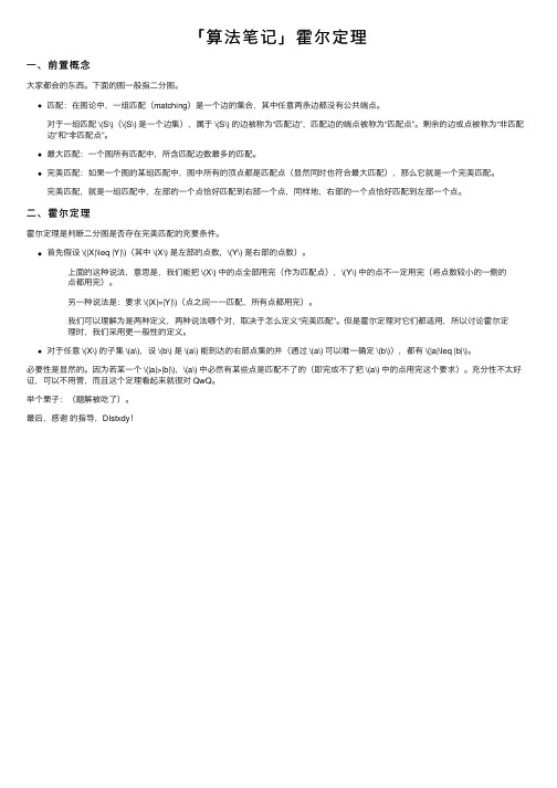
匹配:在图论中,⼀组匹配(matching)是⼀个边的集合,其中任意两条边都没有公共端点。
对于⼀组匹配 \(S\)(\(S\) 是⼀个边集),属于 \(S\) 的边被称为“匹配边”,匹配边的端点被称为“匹配点”。
剩余的边或点被称为“⾮匹配边”和“⾮匹配点”。
最⼤匹配:⼀个图所有匹配中,所含匹配边数最多的匹配。
完美匹配:如果⼀个图的某组匹配中,图中所有的顶点都是匹配点(显然同时也符合最⼤匹配),那么它就是⼀个完美匹配。
完美匹配,就是⼀组匹配中,左部的⼀个点恰好匹配到右部⼀个点,同样地,右部的⼀个点恰好匹配到左部⼀个点。
⼆、霍尔定理霍尔定理是判断⼆分图是否存在完美匹配的充要条件。
⾸先假设 \(|X|\leq |Y|\)(其中 \(X\) 是左部的点数,\(Y\) 是右部的点数)。
上⾯的这种说法,意思是,我们能把 \(X\) 中的点全部⽤完(作为匹配点),\(Y\) 中的点不⼀定⽤完(将点数较⼩的⼀侧的点都⽤完)。
另⼀种说法是:要求 \(|X|=|Y|\)(点之间⼀⼀匹配,所有点都⽤完)。
我们可以理解为是两种定义,两种说法哪个对,取决于怎么定义“完美匹配”。
但是霍尔定理对它们都适⽤,所以讨论霍尔定理时,我们采⽤更⼀般性的定义。
对于任意 \(X\) 的⼦集 \(a\),设 \(b\) 是 \(a\) 能到达的右部点集的并(通过 \(a\) 可以唯⼀确定 \(b\)),都有 \(|a|\leq |b|\)。
必要性是显然的。
因为若某⼀个 \(|a|>|b|\),\(a\) 中必然有某些点是匹配不了的(即完成不了把 \(a\) 中的点⽤完这个要求)。
充分性不太好证,可以不⽤管,⽽且这个定理看起来就很对 QwQ。
举个栗⼦:(题解被吃了)。
最后,感谢的指导,Dlstxdy!。
Dedicated to the memory of
Abstract A facet of the stable set polytope of a graph G can be viewed as a generalization of the notion of an α-critical graph. We extend several results from the theory of α-critical graphs to facets. The defect of a nontrivial, full-dimensional facet v∈V a(v )xv ≤ b of the stable set polytope of a graph G is defined by δ = v∈V a(v ) − 2b. We prove the upper bound a(u) + δ for the degree of any node u in a critical facetgraph, and show that d(u) = 2δ can occur only when δ = 1. We also give a simple proof of the characterization of critical facet-graphs with defect 2 proved by Sewell [11]. As an application of these techniques we sharpen a result of Sur´ anyi [13] by showing that if an α-critical graph has defect δ and contains δ + 2 nodes of degree δ + 1, then the graph is an odd subdivision of Kδ+2 .
Tunnelling and Underground Space Technology
1. Introduction
Stress redistribution during tunneling should be three-dimensional (3D), with the exception of a two-dimensional (2D) plain strain condition. However, ideal assumptions of a circular-shaped tunnel and the 2D condition are typically invoked for the initial analytic solution. This stress distribution solution for a circular tunnel has been reported throughout the last century. Kirsch (1898) solved analytically the distribution of stress and displacement in an unsupported circular tunnel. His solution relied upon elasticity theory, using the plane stress condition with different K0 values. Bray (1967) proposed a theoretical model to permit analysis of the extent of failure, the plastic zone, based on Mohr–Coulomb failure criterion. Ladanyi (1974) discussed stress distribution around a circular opening in a hydrostatic stress field, and within annular failed rock generated in the excavation periphery, using Mohr–Coulomb elasto-plastic theory.
Solving the feedback vertex set problem on undirected graphs
Feedback problems consist of removing a minimal number of vertices of a directed or undirected graph in order to make it acyclic. The problem is known to be NP complete. In this paper we consider the variant on undirected graphs. The polyhedral structure of the Feedback Vertex Set polytope is studied. We prove that this polytope is full dimensional and show that some inequalities are facet de ning. We describe a new large class of valid constraints, the subset inequalities. A branch-and-cut algorithm for the exact solution of the problem is then outlined, and separation algorithms for the inequalities studied in the paper are proposed. A Local Search heuristic is described next. Finally we create a library of 1400 random generated instances with the geometric structure suggested by the applications, and we computationally compare the two algorithmic approaches on our library. Key words: feedback vertex set, Branch-and-cut, local search heuristic, tabu search.
Small ramsey numbers
*
Stanisław P. Radziszowski Department of Computer Science Rochester Institute of Technology Rochester, NY 14623, spr@ Submitted: June 11, 1994; Accepted: July 3, 1994 Current revision: August 28, 1995
2. Classical Two Color Ramsey Numbers We split the data into the table of values and a table with corresponding references. Known exact values appear as centered entries, lower bounds as top entries, and upper bounds as bottom entries. All the critical graphs for the numbers R (k , l ) (graphs on R (k , l ) − 1 vertices without Kk and without Kl in the complement) are known for k = 3 and l = 3, 4, 5, 6 [Ka2], 7 [RK3, MZ], and there are 1, 3, 1, 7 and 191 of them, respectively. There exists a unique critical graph for R (4,4) [Ka2]. There are 4 such graphs known for R (3,8) [RK2], 1 for R (3,9) [Ka2] and 350904 for R (4, 5) [MR5], but there might be more of them.
- 1、下载文档前请自行甄别文档内容的完整性,平台不提供额外的编辑、内容补充、找答案等附加服务。
- 2、"仅部分预览"的文档,不可在线预览部分如存在完整性等问题,可反馈申请退款(可完整预览的文档不适用该条件!)。
- 3、如文档侵犯您的权益,请联系客服反馈,我们会尽快为您处理(人工客服工作时间:9:00-18:30)。
Takustraße7
D-14195Berlin-Dahlem
Germany
Konrad-Zuse-Zentrum
f¨urInformationstechnikBerlin
ANNEGRETW
AGLER
CriticalEdgesinPerfectGraphsand
SomePolyhedralConsequences
641852710111291112910GL(F=)GL(F=)76514
3
2
8
3
3
54
6
72
8
1
1211
109
F