欧拉积分

合集下载

part1ch6欧拉积分学原理

2
B=
λ −1 A, λ +1
C=
λ − 2 B, λ +2
D=
λ −3 C, λ +3
E=
λ −4 D λ +4
etc.
Now for the odd powers there arises :
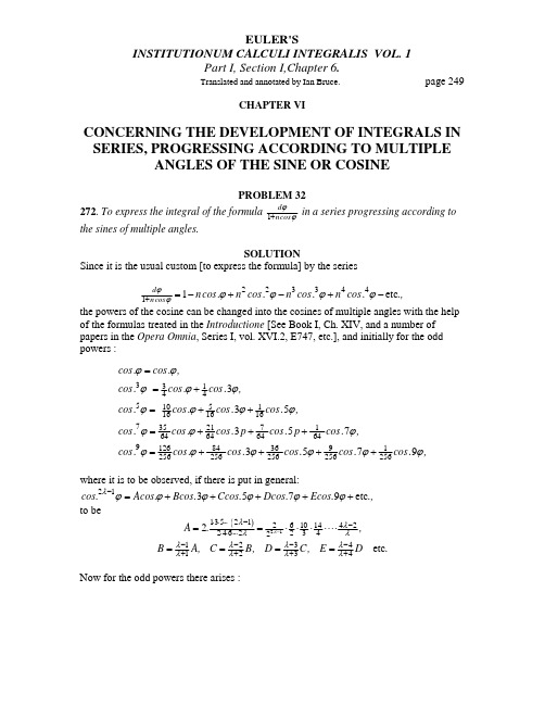
EULER'S INSTITUTIONUM CALCULI INTEGRALIS VOL. 1 Part I, Section I,Chapter 6.
PROBLEM 32 dϕ 272. To express the integral of the formula 1+ ncos in a series progressing according to ϕ the sines of multiple angles. SOLUTION Since it is the usual custom [to express the formula] by the series
B= E=
2 A −1 n 2 D −Cn , n
(
),
C= F=
2 B − 2 An , n 2 E − Dn , n
D= G=
2C − Bn , n 2 F − En , n
etc.
Hence the integral can be assigned easily from these coefficients found; for since there shall be [the integral]
1 (1−nn ) 2 B − 2 A , the recurring series begins again with the term D. Thus edition that since C = n

part1ch4欧拉积分学原理

, and thus it
is reduced towards an algebraic formula, provided that Z should be given algebraically. COROLLARY 2 lx , if there is put lx = u , and U can 191. It is agreed to be noted for the particular case dx x is not difficult, since be some algebraic function of u, the integration of this formula Udx x on account of
∫
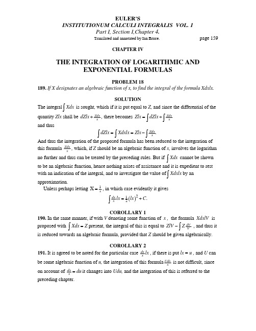
quantity Zlx shall be dZlx + Zdx , there becomes Zlx = dZlx + x and thus
∫
x ∫ Zdx
. x ∫ dZlx = ∫ Xdxlx = Zlx − ∫ Zdx
And thus the integration of the proposed formula has been reduced to the integration of , which, if Z should be an algebraic function of x, involves the logarithm this formula Zdx x no further and thus can be treated by the preceding rules. But if
lx = 1 lx x 2( ) ∫ dx
2
+ C.
COROLLARY 1 190. In the same manner, if with V denoting some function of x , the formula XdxlV is proposed with

part2ch3欧拉积分学原理

− β yXdX + dy (α − X + β XX + y ) = 0
we may have this multiplier
1 y 3 +( 2α − X ) yy +α (α − X + β XX ) y
,
by which that is returned integrable.
EULER'S INSTITUTIONUM CALCULI INTEGRALIS VOL. 1 Part I, Section II, Chapter 3.
Translated and annotated by Ian Bruce.
page 528
1. 2 Pdx + dQ − dM = 0 and
II. PMdx + MdQ − M − II ⋅ 2 produces
− MdQ − MdM + 2α dQ + 2QdM = 0 or
y + Myy + Ny
the common denominator ignored gives : −2 Py 3 − PMy 2 = y 3 + Myy + Ny which following the ordered powers of y gives : 0 = 2 Py 3dx + PMy 2dx + y 3dQ + My 2dQ + NydQ − y 3dM − y 2dN − Qy 2dM − QydN from which the individual powers each are taken to zero, and in the first place we find NdQ − QdN = 0 or

19-3欧拉积分

§3 Euler 积分本节介绍用含参广义积分表达的两个特殊函数 , 即)(s Γ和),(q p B . 它们统称为 Euler 积分. 在积分计算等方面, 它们是很有用的两个特殊函数.一. Gamma 函数 )(s Γ 考虑无穷限含参积分 ⎰+∞--01dx exxs , ) 0 (>s当1 0<<s 时, 点0=x 还是该积分的瑕点 . 因此我们把该积分分为 ⎰⎰+∞+11来讨论其敛散性 .⎰1: 1 ≥s 时为正常积分 .1 0<<s 时, 01>--xs ex.利用非负函数积的Cauchy 判别法, 注意到, 11 , 1) (lim 110⇒<-=---+→s exxxs sx 1 0<<s 时积分⎰1收敛 . (易见 0=s 时, 仍用Cauchy 判别法判得积分发散 ). 因此, 0 >s 时积分⎰1收敛 .⎰+∞1: ) ( , 0112+∞→→=⋅-+--x e x e x x x s x s 对∈∀s R 成立,.因此积分⎰+∞1对∈∀s R 收敛.综上 , 0 >s 时积分⎰+∞--01dx exxs 收敛 . 称该积分为Euler 第二型积分. Euler 第二型积分定义了) , 0 (∞+∈s 内的一个函数, 称该函数为Gamma 函数, 记为)(s Γ, 即)(s Γ=⎰+∞--01dx exxs , ) 0 (>s .Γ函数是一个很有用的特殊函数 .2. -Γ函数的连续性和可导性:)(s Γ在区间) , 0 (∞+内非一致收敛 . 这是因为0=s 时积分发散. 这里利用了下面的结果: 若含参广义积分在] , (b a y ∈内收敛, 但在点a y =发散, 则积分在] , (b a 内非一致收敛 .但)(s Γ在区间) , 0 (∞+内闭一致收敛 .即在任何⊂],[b a ) , 0 (∞+上 , )(s Γ一致收敛 . 因为b a <<0时, 对积分⎰1, 有x a x s e x e x ----≤11, 而积分⎰--11 dx e x x a 收敛.对积分⎰+∞1, xb xs exex----≤11, 而积分⎰+∞--11dx exxb 收敛. 由M —判法, 它们都一致收敛, ⇒ 积分⎰+∞--01dx ex xs 在区间],[b a 上一致收敛 .作类似地讨论, 可得积分dx e x s x s )(10'--+∞⎰也在区间) , 0 (∞+内闭一致收敛. 于是可得如下结论:)(s Γ的连续性: )(s Γ在区间) , 0 (∞+内连续 .)(s Γ的可导性: )(s Γ在区间) , 0 (∞+内可导, 且⎰⎰∞+∞+----=∂∂=Γ'011ln )()(dx x exdx exss xs xs .同理可得: )(s Γ在区间) , 0 (∞+内任意阶可导, 且 ⎰+∞--=Γ01)() ln ()(dxx exs nxs n .3. )(s Γ函数的凸性与极值:0) ln ()(21>=Γ''⎰+∞--dx x exs xs , ⇒ )(s Γ在区间) , 0 (∞+内严格下凸.1)2()1(=Γ=Γ ( 参下段 ), ⇒ )(s Γ在区间) , 0 (∞+内唯一的极限小值点( 亦为最小值点 ) 介于1与2 之间 .4. )(s Γ的递推公式 -Γ函数表:)(s Γ的递推公式 : ) 0 ( ),()1(>Γ=+Γs s s s .证 ⎰⎰+∞+∞--='-==+Γ0)()1(dx ex dx ex s xs xs⎰⎰+∞+∞----∞+-Γ==+-=011)(s s dx ex s dx ex s ex xs xs xs.⎰⎰+∞+∞---===Γ0111)1(dx edx ex xx.于是, 利用递推公式得:1)1(1)11()2(=Γ=+Γ=Γ , ! 212)2(2)12()3(=⋅=Γ=+Γ=Γ,! 3! 23)3(3)13()4(=⋅=Γ=+Γ=Γ , …………, , 一般地有 ! )1()1()()1(n n n n n n n ==-Γ-=Γ=+Γ .可见 , 在+Z 上, )(s Γ正是正整数阶乘的表达式 . 倘定义 )1(! +Γ=s s , 易见对1->s ,该定义是有意义的. 因此, 可视)1(+Γs 为) , 1 (∞+-内实数的阶乘. 这样一来,我们很自然地把正整数的阶乘延拓到了) , 1 (∞+-内的所有实数上, 于是, 自然就有1)1()10(!0=Γ=+Γ=, 可见在初等数学中规定 1!0=是很合理的.-Γ函数表: 很多繁杂的积分计算问题可化为-Γ函数来处理. 人们仿三角函数表、对数表等函数表, 制订了-Γ函数表供查. 由-Γ函数的递推公式可见, 有了-Γ函数在10<<s 内的值, 即可对0>∀s , 求得)(s Γ的值. 通常把00.200.1≤≤s 内-Γ函数的某些近似值制成表, 称这样的表为-Γ函数表 .5. -Γ函数的延拓:0 >s 时, ),()1(s s s Γ=+Γ⇒ .)1()(ss s +Γ=Γ 该式右端在01<<-s 时也有意义 . 用其作为01<<-s 时)(s Γ的定义, 即把)(s Γ延拓到了) , 0 () 0 , 1(∞+⋃-内.12-<<-s 时, 依式 ss s )1()(+Γ=Γ, 利用延拓后的)(s Γ, 又可把)(s Γ延拓到⋃--) 1 , 2 () , 0 () 0 , 1(∞+⋃-内 .依此 , 可把)(s Γ延拓到) , (∞+∞-内除去) , 2 , 1 , 0 ( =-=n n x 的所有点. 经过如此延拓后的)(s Γ的图象如[1] P347图表21— 4.例1 求) 85.4 (Γ, ) 85.0 (Γ, ) 15.2 (-Γ. ( 查表得) 85.1 (Γ94561.0=.) 解 ) 85.4 (Γ=Γ⨯⨯=Γ⨯=Γ=)85.1(85.185.285.3)85.2(85.285.3)85.3(85.3 19506.1994561.085.185.285.3=⨯⨯⨯=. 85.0(85.0) 85.1 (Γ=Γ), ⇒ 11248.185.094561.085.0)85.1() 85.0 (==Γ=Γ.=-Γ⨯=--Γ⋅-=--Γ=-Γ15.0)85.0(15.115.2115.1)15.0(15.2115.2)15.1() 15.2 (54967.215.015.115.294561.0-=⨯⨯-=.6. -Γ函数的其他形式和一个特殊值:某些积分可通过换元或分部积分若干次后化为-Γ函数 . 倘能如此, 可查-Γ函数表求得该积分的值.常见变形有:ⅰ> 令)0( >=p pt x , 有 )(s Γ=⎰+∞--01dx exxs ⎰+∞--=01dtetppts s,因此, ⎰+∞---Γ=01)(s pdx exspxs , ) 0 , 0 (>>s p .ⅱ> 令,2t x = ⇒ ⎰+∞--=Γ01222)(dt e t s t s .注意到[1] P277 E7的结果⎰∞+-=22πdx ex, 得)(s Γ的一个特殊值221=⎪⎭⎫⎝⎛Γ772454.12202≈=⋅=⎰∞+-ππdt et.ⅲ> 令)0( ln >-=λλt x , 得 )(s Γ⎰--⎪⎭⎫⎝⎛=10111ln dttt s sλλ. 取1=λ, 得)(s Γ⎰⎰---=⎪⎭⎫⎝⎛=1111)ln (1ln dtt dt t s s .例2 计算积分 ⎰+∞-022dx exxn, 其中 +∈Z n .解 I ⎰∞++--=-=Γ-⋅=+Γ=====01212!)!12()21(2!)!12(21)21(21212πn n tn xt n n n dt e t.二. Beta 函数),(q p B ——Euler 第一型积分： 1． Beta 函数及其连续性：称( 含有两个参数的 )含参积分⎰---111)1(dx x x q p ) 0 , 0 (>>q p 为Euler 第一型积分. 当p 和q 中至少有一个小于1 时, 该积分为瑕积分. 下证对 0 , 0 >>q p , 该积分收敛. 由于1 , <q p 时点0=x 和1=x 均为瑕点. 故把积分⎰1分成⎰210和⎰121考虑.⎰21: 1≥p 时为正常积分; 10<<p 时, 点0=x 为瑕点. 由被积函数非负,) 0 ( , 1)1(111+---→→-x x x x q p p 和 11<-p ,( 由Cauchy 判法) ⇒ 积分⎰21收敛 . ( 易见0=p 时积分⎰21发散 ).⎰121: 1≥q 时为正常积分; 10<<p 时, 点1=x 为瑕点. 由被积函数非负,) 1 ( , 1)1()1(111----→→--x x x x p q q 和 11<-q ,( 由Cauchy 判法) ⇒ 积分⎰121收敛 . ( 易见0=q 时积分⎰121发散 ).综上, 0 , 0 >>q p 时积分⎰1收敛. 设D }0 , 0 |),( {+∞<<+∞<<=q p q p ,于是, 积分⎰10定义了D 内的一个二元函数. 称该函数为Beta 函数, 记为),(q p B , 即),(q p B =⎰---111)1(dx x x q p ) 0 , 0 (>>q p不难验证, -B 函数在D 内闭一致收敛. 又被积函数在D 内连续, 因此 , -B 函数是D 内的二元连续函数.2. -B 函数的对称性: ),(q p B ),(p q B =.证 ),(q p B =⎰---1011)1(dx x xq p ⎰=--=====---=01111)1(dt tt q p tx⎰=-=--111),()1(p q B dt t tp q .由于-B 函数的两个变元是对称的, 因此, 其中一个变元具有的性质另一个变元自然也具有.3. 递推公式: ) , 1 (1) 1 , 1 (q p B q p q q p B +++=++.证 ⎰⎰=-+=-=+++111)()1(11)1() 1 , 1(p q qp xd x p dx x x q p Bdx x xp q dx x xp q xx p q p q p p q⎰⎰-+-++-+=-++-+=11111111)1(1)1(1)1(11, )*而 ⎰⎰=---=---+11111)1)](1([)1(dx x x x xdx x xq ppq p⎰⎰++-+=---=-111)1 , 1() , 1()1()1(q p B q p B dx x x dx x x qpq p,代入)*式, 有 ) 1 , 1 (1) , 1 (1) 1 , 1 (+++-++=++q p B p q q p B p q q p B ,解得 ) , 1 (1) 1 , 1 (q p B q p qq p B +++=++.由对称性, 又有) 1 , (1) 1 , 1 (+++=++q p B q p p q p B .4. -B 函数的其他形式:ⅰ> 令αx y =, 有 ⎰⎰=-=--1111)1(1)1(dy y y y dx x x αβαγβαγα⎰⎪⎭⎫ ⎝⎛++=-=-+-+111111 , 11)1(1βαγααβαγB dy y y, 因此得 ⎰⎪⎭⎫⎝⎛++=-11 , 11)1(βαγαβαγB dx x x , 1 , 01->>+βαγ. ⅱ> 令x y cos =, 可得⎰⎪⎭⎫ ⎝⎛++=2021 , 2121cos sin πβαβαB xdx x , 1 , 1->->βα. 特别地 , ⎰⎪⎭⎫ ⎝⎛+=2021 , 2121sin πn B xdx n , +∈Z n . ⅲ> 令tt x +=1, 有),(q p B =⎰---111)1(dxx xq p =⎰∞++-+01)1(dt t tqp p ,即 ⎰∞++-=+01),()1(q p B dt t tqp p , ) 0 , 0 (>>q pⅳ> 令ab a ab x t ---=, 可得⎰-+---=--ban m n m n m B a b dx x b a x ),,()()()(111 0 , 0>>n m .ⅴ> ⎰+=+-+--111),()1(1)()1(n m B a a dx x a x xnnnm n m , 0 , 0 ; 1 , 0>>-≠n m a .三. -Γ函数和-B 函数的关系: -Γ函数和-B 函数之间有关系式 )()()(),(q p q p q p B +ΓΓΓ=, ) 0 , 0 (>>q p以下只就p 和q 取正整数值的情况给予证明. p 和q 取正实数值时, 证明用到-Γ函数的变形和二重无穷积分的换序. 参阅[1] P349.证反复应用-B 函数的递推公式, 有 )1 , (112211)1,(11),(m B m n m n n m n n m B n m n n m B +⋅⋅-+-⋅-+-=--+-= ,而 ⎰⇒==-11, 1)1 , (mdx xm B m =--⋅⋅+⋅⋅-+-⋅-+-=)!1()!1(1112211),(m m m m n m n n m n n m B)()()()!1()!1()!1(m n m n n m m n +ΓΓΓ=-+--=.特别地, 0 , 0>>q p 且1=+q p 或2=+q p 时, 由于1)2()1(=Γ=Γ, 就有)()(),(q p q p B ΓΓ=.余元公式——-Γ函数与三角函数的关系：对10<<p ，有 ππp p p sin )1()(=-ΓΓ.该公式的证明可参阅: Фихтенгалъц , 微积分学教程 Vol 2 第3分册, 或参阅余家荣编《复变函数》P118—119 例1（利用留数理论证明）.利用余元公式, 只要编制出210≤<s 时)(s Γ的函数表, 再利用三角函数表, 即可对0>∀s , 查表求得)(s Γ的近似值.四.利用Euler 积分计算积分:例3 利用余元公式计算⎪⎭⎫ ⎝⎛Γ21.解 πππ==⎪⎭⎫ ⎝⎛-Γ⎪⎭⎫ ⎝⎛Γ=⎪⎭⎫ ⎝⎛Γ2sin21121212, ⇒ π=⎪⎭⎫⎝⎛Γ21.例4 求积分⎰∞++061xdx .解令6x t =, 有 I ⎰⎰∞+∞++--=⎪⎭⎫ ⎝⎛=+=+=65611616565 , 6161)1(61161B dt t t dt tt36sin616116161πππ=⋅=⎪⎭⎫ ⎝⎛-Γ⎪⎭⎫ ⎝⎛Γ=.例5 计算积分 ⎰-1441x dx.解 ,2111lim4441=---→xx x 141<=p , ⇒ 该积分收敛 . ( 亦可不进行判敛 ,把该积分化为-B 函数在其定义域内的值 , 即判得其收敛 . )I ⎰⎰⎰=-====-⋅=-⋅=--=141431443414433)1(411)(4114dt t tx x x d xx dx x xt==⎪⎭⎫ ⎝⎛Γ⎪⎭⎫ ⎝⎛Γ=⎪⎭⎫ ⎝⎛=-=⎰--4sin4143414143 , 4141)1(411143141ππB dt t t42π.例6 x x x f 67cos sin )(=, 求积分 ⎰⎰⎰Vdxdydz z f y f x f )()()(,其中 V : x z x y x ≤≤≤≤≤≤0 , 0 , 20π.解 ⎰⎰⎰⎰⎰⎰⎰⎰=⎪⎭⎫ ⎝⎛==Vx xxdx dt t f x f dz z f dy y f dx x f 2220)()()()()(ππ⎰⎰⎰⎰⎰⎪⎪⎪⎭⎫ ⎝⎛=⎪⎭⎫ ⎝⎛=⎪⎭⎫ ⎝⎛=2320232)(31)(31)()(πππxxxdx x f dt t f dt t f d dt t f . 而 ⎰⎰=⎪⎭⎫ ⎝⎛=⎪⎭⎫ ⎝⎛++==226727 , 421216 , 21721cos sin)(ππB B xdx x dx x f 5633)5.0(5.05.15.25.35.45.55.6)5.0(5.05.15.2 !321)215 () 27()4(21.=Γ⨯⨯⨯⨯⨯⨯⨯Γ⨯⨯⨯⨯⋅=ΓΓΓ⋅=. 因此 , 33.)563(9563331=⎪⎭⎫ ⎝⎛=⎰⎰⎰V.。

伽马函数的两种表达式

伽马函数的两种表达式
伽马函数是数学领域中一种非常重要的特殊函数，其应用广泛，例如在物理学、工程学和统计学等领域都有着很重要的作用。

伽马函数有很多种表达式，其中比较常用的有两种表达式：欧拉积分表达式和无穷积表达式。

本文将分步骤对这两种表达式进行阐述。

一、欧拉积分表达式
欧拉积分表达式是伽马函数中最早被发现的表达式，它的形式如下：
Γ(z) = ∫0∞ t^(z-1) * e^(-t) dt
其中，z是伽马函数的参数，t是积分变量。

欧拉积分表达式可以被证明为在定义域内一致收敛的，也就是说，对于任意实数z，都可以用该式子求出其伽玛函数值。

二、无穷积表达式
除欧拉积分表达式外，另外一种常用的伽马函数表达式为无穷积表达式。

其表达式如下：
Γ(z) = 1/ z ∏ n=1∞ [ (1 + 1/n)^(z) * e^(-1/n) ]
其中z为伽马函数的参数，n为自然数。

无穷积表达式是由勒让德在18世纪时提出的，其优点在于对于大多数数值计算机而言，速度要比欧拉积分表达式更快，能够更加精确地计算伽马函数的值。

三、结论
伽马函数在其它各种数学函数中起到积极的作用，是否采用哪一种伽玛函数表达式，主要取决于具体数值计算的需要，或者是所处的数学领域的特点。

总的来说，欧拉积分表达式和无穷积表达式两者都是比较常用的伽马函数表达式，并且都有各自的特殊用处和优点，这在具体应用中要看实际需求而定。

part1ch3欧拉积分学原理

M lx is introduced.
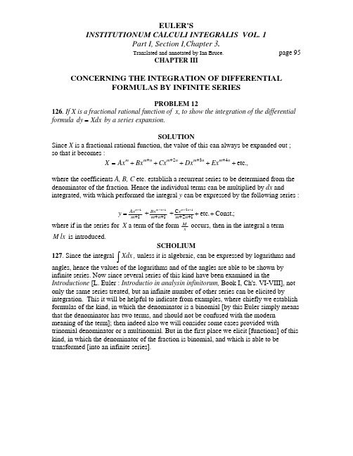
127. Since the integral
∫
SCHOLIUM Xdx , unless it is algebraic, can be expressed by logarithms and
angles, hence the values of the logarithms and of the angles are able to be shown by infinite series. Now since several series of this kind have been examined in the Introductione [L. Euler : Introductio in analysin infinitorum, Book I, Ch's. VI-VIII], not only the same series treated, but an infinite number of other series can be elicited by integration. This it will be helpful to indicate from examples, where chiefly we establish formulas of the kind, in which the denominator is a binomial [by this Euler simply means that the denominator has two terms, and should not be confused with the modern meaning of the term]; then indeed also we will consider some cases provided with trinomial denominator or a multinomial. But in the first place we elicit [functions] of this kind, in which the denominator of the fraction is binomial, and which is able to be transformed [into an infinite series].

part4ch8欧拉积分学原理

Translated and annotated by Ian Bruce. page 1151CHAPTER VIIICONCERNING THE RESOLUTION OF OTHER SECOND ORDER DIFFERENTIAL EQUATIONS BY INFINITESERIESPROBLEM 122967. To show the general form of second order differential equations that it is permitted conveniently to resolve by series, and to investigate the integrals of these.SOLUTIONIn the first place other equations are not able to be resolved by series conveniently, other than those in which the other variable y with its differentials dy and ddy nowhere have dimensions greater than one, since on substituting the infinite series for y we come across great difficulties in the calculations, if greater dimensions should arise anywhere. Hence equations of this kind may be encountered in this form22ddy Mdxdy Nydx Xdx ++=.Then as any term of an assumed series of y can be determined by the preceding one only, which is the most noteworthy case of resolution, it is required for terms of two kinds only to be present in a ratio of the other variable x , since we consider the dimensions which x itself with it differential dx make. From which indeed initially by rejecting the term 2Xdx , the equations may be contained in this form in a resolvable way()()()20n n n xx a bx ddy x c ex dxdy f gx ydx .+++++= For the resolution of this, we put in place23etc n n n y Ax Bx Cx Dx .λλλλ+++=++++and with the substitution made the following sum of the series must be reduced to zero :Translated and annotated by Ian Bruce. page 1152()()()()()()()()()()21 1221etc 1 1 2 n n Aax n n Bax n n Cax .Ab n n BbAc n Bc n Ccλλλλλλλλλλλλλλλλ++−+++−+++−++−+++−++++++() Ae n BeAf Bf CfAg λλ+++++++ BgHence initially here the exponent λ must be taken thus, so that there shall be()10a c f λλλ−++=,then it is necessary for the remaining terms to become :()()()()()()()()()()()()1 1((2)(21)(2))(()1)((3)313) (221(2)) n n a n c f B b e g A,n n a n c f C n n b n e g B,n n a n c f D n n b n e g C λλλλλλλλλλλλλλλλλλ++−+++=−−++++−+++=−++−+++++−+++=−++−+++ etc .Therefore since there shall be (1)0a c f λλλ−++=, if for the case of brevity we put()1b e g h λλλ−++=, there will be((21))(2(221)2)((2l )(3(321)3)(2(221)2) etc n n a nc B hA,n n a nc C n n )b ne h B,n n a nc D n n b ne h C.λλλλλ+−+=−+−+=−+−+++−+=−+−++Hence unless 0a =, because two values are found for λ,λ=clearly two series are found for y , which combined in some manner present the complete integral of the equation.OTHERWISEFor the proposed equationTranslated and annotated by Ian Bruce. page 1153()()()20n n n xx a bx ddy x c ex dxdy f gx ydx ,+++++=a series in reverse order also can be imagined :23etc n n n y Ax Bx Cx Dx .λλλλ−−−=++++,from which there arises on reduction to zero :()()()()()()()()()()1 1221etc 1 1 2 n n Abx n n Bbx n n Cbx .Aa n n BaAe n Be n Ceλλλλλλλλλλλλλλλλ+−−+−−−+−−−++−+−−−++−+−+() Ac n BcAg Bg CgAf λλ+−+++++ BfHence the exponent λ here must be taken thus, so that there is made(l)0b e g λλλ−++=.Then if we put(1)a c f h λλλ−++=,the determination of the coefficients may be considered thus :((21))(2(221))((2l )(3(321))(2(221)2) etc n n b e B hA,n n b e C n n )a nc h B,n n b e D n n a nc h C.λλλλλ−+−=−−+−=−−+−+−+−=−−+−+Translated and annotated by Ian Bruce. page 1154COROLLARIUM 1968. From the first solution, if i should denote some positive integer, the assumed series may terminate somewhere, if there should be [with or without the abbreviation h ]()()()()210 or 10in in b ine h in in b in e g λλλλ+−++=++−+++=,that is(21)(1)0 b in b in in b .e ine g λλλλ+−+−⎫=⎬+++⎭COROLLARY 2969. Hence our equation is allowed to be integrated [with a finite number of terms], if the letters f and g should be prepared thus, so that there shall be(1) and ()(1)()f a c g in in b in e λλλλλλ=−−−=−++−−+,or with two numbers and v μ taken , so that v μ−shall be divisible by the exponent n, if there should be()()1 and 1f a c g v v b ve μμμ=−−−=−−−.COROLLARY 3970. Hence since there shall bev μ== the equation will be considered an algebraic integral, if there should be v in μ−= with i denoting a positive whole number, that is, if there should be22c e a b in =−±COROLLARY 4971.But if it should come about that the exponent λfor the series becomes imaginary, itis agreed to be noted that()x x e x cos.lx lx ,αααββ+==+from which the two series thus can be combined, so that the integral may follow a real form.Translated and annotated by Ian Bruce. page 1155SCHOLIUM972. Each solution generally considered supplies a twofold series for the variable y for the twin values of the exponent λ, the combination of which shows the complete integral. Clearly the first solution for the exponent λ gives these two valuesλ=the latter solutionλ=thus so that in this manner the complete integral can be expressed in two ways. Which two forms even if greatly different and thus meanwhile the one progressing by imaginary exponents, while the other has real exponents, yet they must be equivalent to each other[Recall that the first series is expressed in ascending powers of x while the second series is expressed in descending powers of x ; Euler will treat mainly the ascending case in what follows, and he is most interested in the cases in which some 'inconvenience' arises between the values of λ found in the indicial equation, usually resulting in an infinite term in a series.]Also since it may come about, that either solution or both may show a nonsensical complete integral, while a single series is sufficient [for a particular integral]. This inconvenience for each solution can happen in two ways; certainly for the first solution, where the exponent λ is required to be defined from this equation()10a c f λλλ−++=, then it is elicited from a single value for λ, if there should beeither 0a = or 24()af a c =−. Only in the first case there shall be f cλ=−, in the other case the value of λ becoming as if infinite, now in the second case both values of λbecome equal to each other, clearly 2a c a.λ−= The same inconvenience has to be considered in the other solution, if there should be either b = 0 or 24()bg b e =−, from which it becomes apparent that one solution labours under this inconvenience, while the other is free from that, as also each indeed iscorrupted by the same. On account of which that may be appropriate to be shown, as the complete integral must be investigated in these cases also; with which view also we refer to the case in which both the values of λ become imaginary, since it is necessary to remove the imaginary kind by a particular trick. Now finally also the two series for y shown are difficult to put into use, whenever the values of λare divisible by a different exponent n , the setting out of which cases also is worth explaining.Translated and annotated by Ian Bruce. page 1156PROBLEM 123973. For the proposed second order differential equation()()()20n n n xx a bx ddy x c ex dxdy f gx ydx +++++=,if it comes about that the two ascending series assumed for y either merge together into one, or the other series becomes impossible, to express the complete integral by series.SOLUTIONWith the series assumed23etc n n n y Ax Bx Cx Dx .λλλλ+++=++++if it should come about, that both the values of λ from the equation()10a c f λλλ−++=either become equal or they maintain a difference divisible by n , [which is a degenerate case] then the value of y besides the powers of x also involves the logarithm of x . Whereby [§ 934] for the resolution of the equation we put at once y u vlkx =+, so that y u vlx v α=++with αdenoting some constant quantity. Hence there shall be22 and vdx dxdv vdx x x xxdy du dvlkx ddy ddu ddvlkx =++=+−+,with which values substituted our equation adopts this form2222()2()() ()( ( (()(())n n n n n n n n n xx a bx ddu x a bx dxdv a bx vdx x c ex dxdu c ex )vdx f gx )udx xx a bx ddv x c ex )dxdv f gx vdx lkx ⎫+++−+⎪⎪++++⎬++++++++0,=⎪⎪⎭where the final part affected by the logarithm must separately be equal to zero. Whereby on putting23etc n n n v Ax Bx Cx Dx .λλλλ+++=++++Translated and annotated by Ian Bruce. page 1157that value is attributed to the exponent λfrom the equation ()10a c f λλλ−++=, which is in no manner inconvenient, and for the remainder of the coefficients there will be on putting()1b e g nh λλλ−++=,so that there follows,((21)) 02((221))((21))03((321))2((221))04((421))3((321))0etc n a c B hA ,n a c C n b e B hB ,n a e E n b e C hC ,n a e E n b e D hD .λλλλλλλ+−++=+−+++−++=+−+++−++=+−+++−++=Thus with these coefficients defined, the first of which A is left to our choice, we may put23etc n n n u x x x x .λλλλΔ+++=+++++A B C Dwhich value if substituted into the first equation with the series found for v , the following series is required to be reduced to zero :()()()()22 ()()()l ()(n l)(2)(2l)etc 1 21 n n n dd d dx dxn n xx a bx x c ex f gx ax n ax n n ax .b n n bc ΔΔλλλΔλλλλλλλλλλλ++++++++−+++−+++−++−+++−++A B C A B A () () (2) n c n ce n ef f λλλλ+++++++++B C A B A B ()() 2 2 22 fg gAa n Ba n Caλλλ+++++++C A B ()()2 2() () (Ab n BbA c aB c aC c a A e b λλ++++−+−+−+−()) B e b +−But since there shall be ()10a c f λλλ−++=and ()1b e g nh λλλ−++=, the expression will be transformed into this formTranslated and annotated by Ian Bruce. page 1158()()()()()()()2221 ((221)) ((421) ) etc.2 1 ((2 21)) ((21))2((221)) n n n dd d dx dx n n xx a bx x c ex f gx a c Ax n a c Bx n a c Cx b e A n b e Bn n a c n n a e λΔΔλλΔλλλλλλλ++++++++−+++−+++−+++−+++−+++−+++−++ B C((21)) nh n n b e nh λ++−++A BBwhere Δ denotes certain terms of the seriesetc n x x .λλ+++A Bto be put in place, thus so that in the reverse order there shall be23n n n in x x x .......x .λλλλΔ−−−−++++=a b c iBecause a starting condition has to be put in place for any case, the following are to be observed.I. A starting term cannot be put in place, unless there should be()(l)()0in in a in c f λλλ−−−+−+=;therefore since ()10a c f λλλ−++=, then there shall bein λ=+and henceλ=since these two values cannot agree, unless the sign for the negative root in the former, is taken as positive in the latter. But with these values of the equation there shall be()2or 4in iinnaa a c af ==−−Translated and annotated by Ian Bruce. page 1159and hence ()2144a c a f iinna −=−, from which there becomes 122a c a in λ−=+.Whereby if the proposed equation should be prepared thus, so that there shall beina =then on taking122a c a in λ−=+ and for the series v takingetc n v Ax Bx λλ+=++.it is agreed thus to establish for the other series u :2 etc in n n n u x ...x x x x λλλλλ−−++=++++++i a A B C .This is the case in which the two values of λ from the equation ()10a c f λλλ−++= have a difference divisible by n , where it is to be observed that the series v must start from a greater value of λ, truly the series u must start from a lower value.II. The starting term Δ cannot be omitted, unless there should be (21)0a c λ−+=, in which case there becomes 2a c λ−= ; and this is the case in which the two roots of theequation ()10a c f λλλ−++= become equal to each other, and thus ()24a c a f .−= Hencethis case can be contained in the preceding on taking there 0i =.Whereby in this manner the cases may be resolved, in which the two values of λ either are equal to each other or they have a difference divisible by n . And thus the complete integral is found for the two ascending series v et u expressed, of which that one v is multiplied by lx .COROLLARY 1974. Hence when the coefficients a, c and f thus have been prepared in the proposed equation, so that the roots of the equation ()10a c f λλλ−++= areand in λμλμ==− , with i denoting some positive integer, the complete integral of this kind will have the form y u av vlx =++.Translated and annotated by Ian Bruce. page 1160COROLLARY 2975. But here the two quantities v and u thus can be determined from these equations :()()()2I 0n n n .xx a bx ddv x c ex dxdv f gx ydv +++++=()()()()222II 2 0 (n n n n n n .xx a bx ddu x c ex dxdu f gx udx x a bx dxdv (a bx )vdx ,c ex )vdx ⎫+++++⎪⎪++−+=⎬⎪⎪++⎭as there is put2323 etc etc n n n in in n in n in n v Ax Bx Cx Dx .,u x x x x .μμμμμμμμ+++−−+−+−+=++++=++++A B C DEvidently these series on being substituted all the coefficients are allowed to be defined except one.SCHOLION976. Hence with the logarithm of x called into help in these cases that we havementioned, the complete integral of the proposed equation can be shown by an ascending series, while without this artifice only a particular integral can be found. For when the equation ()10a c f λλλ−++= has two roots, the difference of which is divisible by the exponent n , for example and in λμλμ==−, by the first method only the series, which starts with the power x μ, is able to be determined ; for if the other starting from the power in x μ−is assumed for y , the coefficient of a certain term is found to be infinite, from which all the following terms become infinite too, which inconvenience onintroducing the logarithm of x is happily removed. Therefore it will be helpful to make clear the use of this resolution by a few examples.Translated and annotated by Ian Bruce. page 1161EXAMPLE 1977. To show the complete integral of the second order differential equation120n xddy dxdy gx ydx −++=by an ascending series.We will have this equation 20n xxddy xdxdy gx ydx ,++= on reducing our form, where hence there shall be 1010and 0a ,b ,c ,e ,f =====. Hence()10or 0λλλλλ−+==, thus so that the two values of λ are equal and = 0.Whereby on putting y u v vlx α=++ these equations must be resolved2I 0n .xxddv xdxdv gx vdx ++=and2II 0 2 n .xxddu xdxdu gx udx xdxdv ⎫++⎪=⎬+⎪⎭Hence we put in place23etc n n n v A Bx Cx Dx .=++++and23etc n n n u x x x .=++++A B C Dand the first equation gives()()()231221331etc 2 3 0 n n n n n Bx n n Cx n n Dx .nB nC nD ,Ag Bg Cg ⎫−+−+−+⎪⎪+++=⎬⎪+++⎪⎭from which there shall be4916, , etc Ag Bg Cg Dgnn nn nn nn B C D ,E .−−−−====Then indeed the other equation gives2349etc. 02 4 6n n n nn x nn x nn x g g g ,nB nC nD⎫+++⎪+++=⎬⎪+++⎭B C D A B Cfrom which there is deduced2224293,,,etc g g g C B Dnn n nn n nnn ,.−−−=−=−=−A B A B C DTranslated and annotated by Ian Bruce. page 1162But here it is allowed to assume without risk that 0=A , because the terms arising from A are contained in the part v α. Therefore since there shall be344681414914916, ,etc Ag Agg Ag Ag nnn n n B C ,D E .,−+−+⋅⋅⋅⋅⋅⋅====there will be, as follows,35553334449995511222642142146222214931492314922210023149164149162314916100223414916255149162== ,AgAgg Agg Aggnn n n Ag Ag Ag n n n Ag Ag Ag n n n Ag Ag n ,,,−−⋅⋅⋅⋅⋅⋅⋅⋅⋅⋅⋅⋅⋅⋅−−⋅⋅⋅⋅⋅⋅⋅⋅⋅⋅⋅⋅⋅⋅⋅⋅⋅⋅⋅⋅⋅⋅⋅⋅⋅⋅==−==+=−=+B A D E F 51111548523451491625 etc Ag n n .⋅⋅⋅⋅⋅⋅⋅⋅=and thus the following values may be obtained :3456111326221001818271827645483528182764125182764125216,etc Ag Agg Ag Ag n n n n Ag Ag n n ,,,,.,−−⋅⋅⋅⋅⋅⋅−⋅⋅⋅⋅⋅⋅⋅⋅⋅======B C D E E Gwhere the individual numerators 2, 6, 22, 100, 548, 3528 etc. thus are defined by the two preceding63210 225642 1007229654891001622 35281154825100 etc ,,,,.=⋅−⋅=⋅−⋅=⋅−⋅=⋅−⋅=⋅−⋅Consequently the integral is expressed thus :()3435793446634468262210023418182718276423414149149162341414914916etc 1 etc etc Ag AggAg Ag nnnn n n n n g gg g g n nnn nnnn n gggg g nnnnnnnnny x xxx .A x xxx .lx x xx x .ααααα⋅⋅⋅⋅⋅⋅⋅⋅⋅⋅⋅⋅⋅⋅⋅⋅⋅⋅=−+−++−+−+−+−+−+−where A and a are two arbitrary constants.Translated and annotated by Ian Bruce. page 1163EXAMPLE 2978. To assign the complete integral of the second order differential equation()21(1)0x xx ddy xx dxdy xydx −−++=by an ascending series.Our equation is reduced to the form()21(1)0x xx ddy xx dxdy xydx −−++=,thus, so that there shall be 21 1 1 10 and 1n ,a ,b ,c ,e ,f g ===−=−=−==, from which the roots of the equation ()10λλλ−−=shall be 0 et 2λλ==, the difference of whichdivided by 2n = gives 1. Hence on putting y u v vlx α=++ there must be put in place2468etc v Ax Bx Cx Dx .=++++and2468etc u x x x x .=+++++A B C D Ewhich series must be determined from the following equations :2I (1)(l 0.xx xx ddv x xx )dxdv xxvdx ,−−++=22II (1)(l )2(1)20.xx xx ddu x xx dxdu xxudx x xx dxdv vdx .−−+++−−=Hence for the determination of the first there becomes24682123056 etc 2 12 302 4 6 8 0 2 4 6 Ax Bx Cx Dx .A B C A B C D A B CA B C ⎫++++⎪−−−⎪⎪−−−−=⎬⎪−−−⎪+++⎪⎭and thus2413 4635 6857 etc B A,C B,D C .⋅=⋅⋅=⋅⋅=⋅or131335133557242446244668 etc B A,C A,D A .⋅⋅⋅⋅⋅⋅⋅⋅⋅⋅⋅⋅⋅⋅⋅⋅⋅⋅=== Now there is found from the other equationTranslated and annotated by Ian Bruce. page 116424682123056 etc 2123024 6 8 2 4 6 4 8 12 16 4 8 12x x x x .A B C D A B ++++−−−−−−−−−−++++++++−−−B C D E B C D B C D EB C D A B C D 02 2 2 2,C A B C D ⎫⎪⎪⎪⎪⎪=⎬⎪⎪⎪⎪⎪−−−−⎭from which there is required to become202413640 46351080 685714120 etc A ,B A ,·C B ,D C .,+=⋅−⋅+−=⋅−+−=⋅−⋅+−=A C B D C E Dor since there shall be133557244668etc B A,C B,D C .,⋅⋅⋅⋅⋅⋅=== there shall be 2A =−A , then indeed2222222227132724242435221221464646243572436868682737927381081081024 1304635068 570810790A ,A,B ,B,C ,C,D ,D ⋅⋅⋅⋅⋅⋅⋅⋅⋅⋅⋅⋅⋅⋅⋅⋅⋅⋅⋅⋅⋅⋅⋅⋅⋅−⋅−==+⋅−⋅−==+⋅−⋅−==+⋅−⋅−==+C B C B D C D C E D E D F D F E etc.While therefore there may be taken 2A =−A , nothing hinders the letter B from taking any value it pleases, and it may be put equal to zero, if indeed the constant αabove has been introduced.Translated and annotated by Ian Bruce. page 1165EXAMPLE 3979. To show the complete integral of the second-order differential equation2(1)(5)(5)0xx bxx ddy x exx dxdy gxx ydx ++−+++=by an ascending integral.Because here there is 1 5 and 5a ,c f ==−=, the equation (1)550λλλ−−+=or 650λλλ−+=has the roots 1 and 5λλ==, the difference of which 4 can be divided by 2n =. Hence on putting y u v vlx α=++there is put in place5791113etc v Ax Bx Cx Dx Ex .=+++++and357etc ;u x x x x .=++++A B C Dthe equations to be resolved will be2I(1)(5)(5)0.xx bxx ddv x exx dxdv gxx vdx ++−+++=and222II. (1)(5)(5) 2(1)(1) 0 (5)xx bxx ddu x exx dxdu gxx udx x bxx dxdv bxx vax ,exx vdx ⎫++−+++⎪⎪++−+=⎬⎪+−+⎪⎭where the former leads to57911 5476981110 etc 55 57 59 511 5 5 5 5 54 76 98 5 7 9 Ax Bx Cx Dx .A B C D A B C D Ab Bb Cb Ae Be Ce⋅+⋅+⋅+⋅+−⋅−⋅−⋅−⋅+++++⋅+⋅+⋅+++0 ,Ag Bg Cg ⎫⎪⎪⎪⎪=⎬⎪⎪⎪+++⎪⎭the latter toTranslated and annotated by Ian Bruce. page 11663579 23 45 67 89 etc 553 55 57 595 5 5 5 5 23 45 67 x x x x .x i b b b e +⋅+⋅+⋅+⋅+−−⋅−⋅−⋅−⋅++++++⋅+⋅+⋅++B C D E A B C D E A B C D EB C D A 3 5 7 25 27 296 6 6 e e eg g g g A B C A B C +++++++⋅+⋅+⋅−−−B C D A B C D 25 27 Ab Bb Ab BbAe Be ⎫⎪⎪⎪⎪⎪⎪⎪⎪⎬⎪⎪⎪+⋅+⋅−−++⎭0.=⎪⎪⎪⎪⎪ From thence there becomes()()()()()()12 2050 or 26 4550324270 48 6770607290 6108990etcB A b e g B A b e g ,C B b e g C B b e g ,D C b e g D C b e g .+++=⋅+⋅++=+++=⋅+⋅++=+++=⋅+⋅++= etc .But hence()400 (233)4026 (455)8 (9)048 (677)12(13)0 etc e g ,b e g A ,b e g B A b e ,.b e g C B b e .−++=+⋅+++=⋅+⋅+++++=⋅++++++=B A C B D C E DFrom the former formulas the letters B, C, D etc. are determined by A , from the latter thesecond becomes 4A −=B , but from the first 4e g +=A A , then truly C can be for any it pleases to assume and then the remaining coefficients ,,D E F etc. are defined.Translated and annotated by Ian Bruce. page 1167SCHOLIUM980. This example supplies us with the opportunity to observe certain unusualphenomena. Evidently even if the complete integral in general involves lx , yet that produces certain cases free from logarithms.Certainly in the first place if there should be g e =−, there becomes 0=B with A remaining undefined, then truly on account of 0=B it is required to take 0 0A ,B ==etc. and thus 0v =. Again indeed there shall be264(5)0486(7)06l08(9)0 etc b e ,b e ,b e .,⋅++=⋅++=⋅++=D C E D F Ewhere C is an arbitrary constant, and the complete integral of the equation2(1)(5)(5)0xx bxx ddy x exx dxdy exx ydx ++−++−=will be57911etc ,y x x x x x .=+++++A C D E Fwhich thus is expressed finitely if (25)e i b =−+ by taking for i the numbers 0, 1, 2, 3, 4 etc.In the second case if there shall be12330 or 63there becomes (3b )b e g g b e,e ⋅++==−−=−+B A , then truly 000A ,B ,C === etc., hence 0v =. Again indeed there is found111(7)(9)(11)b e ,b e ,b e =−+=−+=−+D C E D F E etc. and hence()3579123etc ,y x b e x x x x .=−+++++A A C D E where and A C remain for our arbitrary constants.In the third place if there shall be 455 0 or 205b e g g b e ⋅++==−−, in the first place there becomes 00 0B ,C ,D === etc. and thus 5v Ax =, then truly27(5)(142)40 or A b e b e ,b e A +=−+−++==B A B B and hence12(5)(7)A b e b e ,=−++A againTranslated and annotated by Ian Bruce. page 1168()()26 904821106104(13) 0 etc A b e ,b e ,b e .⋅++=⋅++=⋅++=D E D F EHence the coefficients etc ,A,,,.B D E F are defined by A , and C too remains for our arbitrary constant, from which the complete integral in this case will be55379etc ,y Ax lx x x x *x x .=+++++++C A B D Ewhich expression becomes finite, whenever (25)0i b e ++=.EXAMPLE 4981. If there shall be in the first example 7 15e b and g b =−=,2(l )(57)5(13)0xx bxx ddy x bxx dxdy bxx ydx +−+++= to show the complete integral of the equation.Hence there shall be 2 0 0 0b,A ,,====B A D E and thus 0v = and352u x bx x ,=++A A Cfrom which on taking some constants for and A C there will be the complete integral()512y x bxx x .=++A C Hence there will be the particular integrals52(12) (1)y ax bxx ,y ax ,y ax bxx .=+==+COROLLARY 1982. On putting zdx y e ∫=, so that there becomes dyydx z =, the complete integral of this first order differential equation(1)(1)(57)5(13)0xx bxx dz xx bxx zzdx x bxx zdx bxx dx +++−+++=will be45(16)5(l 2)bxx x x bxx x z .++++=A C A CTranslated and annotated by Ian Bruce. page 1169COROLLARY 2983. But the equation of the second order differential equation is reduced, if it is divided by 2(1)xx bxx +, and the integral will be55(l ) or (1)xdy ydx ydxx bxx xCdx dy Cdx bxx ,−+=−=+ which divided by 5x gives the integral54251442or (1+2)y C bC xxxD y Cx bxx Dx −=−+=−+ as before.SCHOLIUM984. But at this stage the complete integration of our equation by ascending series fails in the case, in which 0a =and thus 0c f λ+=, from which one value for the exponent λis defined f cλ−=, which supplies only a particular integral, and this also is removed, ifthere should be 0c =. Because moreover in these cases a is = 0, it is necessary that the coefficient b certainly be present, from which the complete integral can be shown by descending powers, since the equation (1)0b e g λλλ−++=always contains two roots, from which the twofold series may be obtained. But likewise here an inconvenience in the use can come about, when the two roots of λ are either equal or they have a difference divisible by the exponent n . Now for this inconvenience on introducing a series multiplied by lx in a like manner a cure is brought about, which we have used in solving this problem, and it would be superfluous to repeat that derivation here. But if moreover the two roots of λboth for the ascending as well as the descending seriesbecome imaginary, that remains to be shown, how the complete integral is required to be expressed by infinite series.Translated and annotated by Ian Bruce. page 1170PROBLEM 124985. For the proposed second order differential equation2()()()0n n n xx a bx ddy x c ex dxdy f gx ydx +++++=if it should come about, that the equation ()10a c f λλλ−++= should have imaginaryroots, to show the complete integral by an ascending series.SOLUTIONFrom the solution produced above (§ 971), it is deduced in this case that there must be put in placesin cos y v .lx u .lx μμ=+,from which there becomes()sin (cos udx vdxx x dy dv .lx du ).lx μμμμ=−++ and222222(+)sin (cos ;dxduudx vdx x xxxxdxdv vdx udx xxxxxddy ddv .lx ddu ).lx μμμμμμμμμμ=−−++−−with which substitution made if we reduce separately both the terms affecting sin as well as cos .lx .lx μμ to zero, we will obtain the following equations :222I () () () 2()() () n n n n n n .xx a bx ddv x c ex dxdv f gx vdx x a bx dxdu a bx vdx a bx udx μμμμ+++++−+−+++20 ()n ,c ex udx μ⎫⎪⎪=⎬⎪⎪−+⎭222II () () () 2()() () n n n n n n .xx a bx ddu x c ex dxdu f gx udx x a bx dxdv a bx udx a bx vdx μμμμ+++++++−+−+20 ()n .c ex vdx μ⎫⎪⎪=⎬⎪⎪++⎭ Now we assume these ascending series for v and uTranslated and annotated by Ian Bruce. page 11712323etc etc n n n n n n v Ax Bx Cx Dx .,u x x x x .λλλλλλλλ++++++=++++=++++A B C Dand with these substituted the first equation will go into this :()()()()()()()()()()211221etc 0 1 1 2 n n Aax n n Bax n n Cax .Ab n n BbAc n Bc n Ccλλλλλλλλλλλλλλλλ++−+++−+++−+=+−+++−+++++() Ae n BeAf Bf Cfλλ+++++++ Ag Bg+2 2() 2(2) 2 2() a n a n ab n bAa B μλμλμλμλμλμμμμ−−+−+−−+−−A B C A B a CaAb Bb a a μμμμμμμμ−−−+++A B ab bc c cμμμμμμ++−−−C A B A B C e eμμ−−A BHence the other equation is easily formed by permuting the latin and gothic letters and by changing the sign of μin addition.Hence the first power x λ removes these equations()()( 1)(2)0( 1)(2)0A a c f a a a c ,a c f a A a a c ,λλλμμμλλλλμμμλ−++−−−+=−++−+−+=A Afor which it is necessary that there shall be both20a a c λ−+=as well as(1)0a c f a λλλμμ−++−=.Thence there becomes 122c a λ=−, which value substituted here givesTranslated and annotated by Ian Bruce. page 117214422424( ) cc c cc a c cc aa a aa f a f μμ−−+−+==−+−+ or()2442and thus af a c a c a aa .μμμλ−−−===From which it is apparent that this solution has to be considered, if 24()af a c >−, in which case the preceding solution becomes imaginary [§ 967] . But here the quantities A and A are left arbitrary in our equation.Now the term n x λ+ demands these equations on both sides :()()()()()()1()l 2()(2)0B n n a n c f a A b e g b n a a c b b e λλλμμλλλμμμλμλ++−+++−+−++−−+−+−−+=B A and()()()()()()(1)()l 2(2)0n n a n c f a b e g b B n a a c A b b e .λλλμμλλλμμμλμλ++−+++−+−++−++−++−+=B AFor the sake of brevity let()()1()n n a n c f a ,λλλμμα++−+++−=()l b e g b ,λλλμμβ−++−=()22n a a c na ,λγ+−+==2b b e λδ−+=,so that we may have0and 0B A B A ,αβμγμδαβμγμδ+−=+++=B -A B Afrom which there is deduced()()()() and A A B .αβμμγδμαδβγαβμμγδμαδβγααμμγγααμμγγ−++−−+−−++==A A B But now from the assumed values there is()()2ae bc a c bf ae bc nna,g,na,,αβγδ−−−==−+==from which the assumed values A and A there are defined B and B and hence again ,C,D,C D etc.。

欧拉积分伽马函数报告

欧拉积分伽马函数报告
欧拉积分伽马函数是一种常用的数学函数，它可以用来描述物理系统中的动力学行为。

它是一种非常有用的工具，可以用来描述物理系统中的动力学行为，以及求解复杂的微分方程。

欧拉积分伽马函数的定义是：它是一种特殊的函数，它可以用来描述物理系统中的动力学行为，它可以用来求解复杂的微分方程。

欧拉积分伽马函数的应用非常广泛，它可以用来求解复杂的微分方程，以及描述物理系统中的动力学行为。

它可以用来解决物理学中的许多问题，如动力学，热力学，电磁学，量子力学等。

此外，它还可以用来解决数学中的许多问题，如求解积分，求解微分方程，求解拟牛顿方程等。

欧拉积分伽马函数的优点是它可以用来求解复杂的微分方程，以及描述物理系统中的动力学行为。

它的缺点是它的计算复杂度较高，而且它的计算结果可能不太准确。

总之，欧拉积分伽马函数是一种非常有用的工具，它可以用来求解复杂的微分方程，以及描述物理系统中的动力学行为。

它的优点是它可以用来求解复杂的微分方程，以及描述物理系统中的动力学行为，但是它的计算复杂度较高，而且它的计算结果可能不太准确。

反向欧拉积分

反向欧拉积分全文共四篇示例，供读者参考第一篇示例：欧拉积分是微积分中的一个重要概念，是对定积分的一种推广形式。

但是在实际问题中，有时候我们也会遇到反向欧拉积分的情况。

反向欧拉积分是什么？它又有什么应用场景呢？让我们先回顾一下欧拉积分的定义。

对于一个函数f(x)，它的欧拉积分可以表示为：\[F(x) = \int_{0}^{x} f(t) dt\]在这个积分中，我们将函数f(x)在区间[0, x]上的取值全部加起来，得到了函数F(x)。

而反向欧拉积分则是反过来，已知一个函数F(x)，我们要找到函数f(x)。

也就是说，我们要找到一个函数f(x)，使得它的欧拉积分等于给定的函数F(x)。

那么反向欧拉积分的应用场景是什么呢？一个典型的例子就是在信号处理中的还原。

在信号处理中，我们经常会遇到信号的积分和微分运算。

如果我们已知一个信号的积分，我们希望能够找到原始的信号，这时候就需要用到反向欧拉积分。

在具体的计算中，我们可以采用不定积分的方法来求解反向欧拉积分。

即我们首先找到函数F(x)的一个反导函数G(x)，即G'(x) = F(x)，然后我们就可以得到f(x) = G'(x)。

举个例子来说，假设我们有一个函数F(x) = 2x^3，我们现在想要找到对应的原函数f(x)。

我们首先求F(x)的反导函数为G(x) =\frac{2}{4}x^4 = \frac{1}{2}x^4，然后我们就可以得到f(x) = G'(x) = x^4。

通过这个例子，我们可以看到反向欧拉积分的过程其实是很简单的，只需要利用不定积分的方法求解即可。

在实际应用中，反向欧拉积分可以帮助我们还原信号，解决问题，提高效率。

反向欧拉积分是欧拉积分的一个重要推广形式，它在信号处理、控制理论、微积分等领域都有重要应用。

通过对反向欧拉积分的了解，我们可以更好地理解微积分的概念，解决实际问题，提高工作效率。

希望这篇文章能帮助大家更深入地了解反向欧拉积分的概念和应用。

part2ch7欧拉积分学原理

EULER'SINSTITUTIONUM CALCULI INTEGRALIS VOL. 1Part I, Section II, Chapter 7.Translated and annotated by Ian Bruce. page 747CHAPTER VIICONCERNING THE APPROXIMATEINTEGRATION OF DIFFERENTIAL EQUATIONSPROBLEM 85650. To assign an approximate value to the complete integral of any differential equation.SOLUTIONLet x and y be two variables, between which the differential equation is proposed, and this equation shall have a form of this kind, so that dydxV =with V being some function of x and y . Now since the complete integral is desired, this has to be interpreted thus, so that while x is given a certain value, for example x a =, the other variable y is given a certain value, for example y b =. Hence in the first place we are to treat the question, so that we can find the value of y, when the value of x is attributed a value differing a little from a , o on putting x a ω=+ so that we may find y. But since ω shall be the smallest possible amount, the value of y will differ minimally from b ; from which, while x only is changed from a as far as to a ω+, the quantity V is allowed to be looked on as being constant. Whereby on putting x a = and y b = there is made V A = and from this very small change we will have dy dxA =and thus on integrating, ()y b A x a ,=+− clearly with a constant of this kind to be added so that on putting x a = there becomes y b =. Hence we may put in place x a ω=+ and there becomes y b A ω=+.Hence just as here from the values given initially x a = and y b = we find approximately the following x a ω=+ and y b A ω=+, thus from these in a like manner it is allowed to progress through another very short interval, as long as it arrives finally at values however far from the starting value. Which operations are put in place so that they appear clearer, are put in place in the following manner successively.The values of successivex IV a,a',a'',a''',a ...'x,xy IV b,b',b'',b''',b ...'y,y b,V IV A,A',A'',A''',A ...'V ,V.Clearly from the first given x a = and y b = there is had V A =, then truly with the following there will be ()b'b A a'a =+− with the smallest difference a'a − assumed as you wish. Hence on putting x a'=and y b'=there is deduced V A'= and from which for the third there will be obtained ()b"b'A'a"a'=+−, where on putting x a"=and y b"=EULER'S INSTITUTIONUM CALCULI INTEGRALIS VOL. 1Part I, Section II, Chapter 7.Translated and annotated by Ian Bruce. page 748there is found V A"=. Now for the fourth we shall have ()b'''b"A"a"'a"=+− and hence on putting x a'"= and y b'''= we may deduce that V A'"= and thus it is permitted to progress to values however distant from the start. Moreover the series showing the successive first values of x as you please can be taken, while in the interval it may either increase or decrease.COROLLARY 1651. Hence for the individual smallest intervals, the calculation is put in place in the same manner and thus the values, upon which the series depends , may be obtained. Hence in this way with the individual values assumed for x the corresponding values of y are able to be assigned.COROLLARY 2652. Because with smaller intervals taken, through which the values of x are assumed to progress, from that more accurate values for the individual points are elicited. Yet meanwhile the errors in the individual points are joined together, and even if they are much smaller, on account of the multitude of these they add up.COROLLARY 3653. But the errors in this calculation thence arise, because in the individual intervals we regard both the quantities x and y as constants and thus the function V may be had as constant. From which hence the more the value of V in some interval following is unchanged, from that the greater the errors are to become worried about.SCHOLIUM 1654. This inconvenience first occurs, when the value of V either vanishes or increases to infinity, even if the changes happening to x and y should be small enough. But from these cases anyhow to avoid falling into immense errors proceed in this manner. For the start of this interval let there be x a = and y b =, then there is put x a ω=+ and y b ψ=+ into the proposed equation, so that there becomes d V ψω=, moreover on V becoming thus on substituting x a ω=+ and y b ψ=+, in order that the quantities and ωψ are considered as very small, clearly on rejecting the higher powers before the lower ones; for in this way generally an integration for these intervals actually can be put in place. But there will scarcely be a need for this improvement, unless the terms arising from the values of a and b cancel each other. Just as if there should be this equation :yydy aa dx xx −=and for the initial term there must be and x a y a ==; now for the start of this interval there is put x a ω=+ and y b ψ=+ and there will be found :2 2a d aa d a ψωωψ−=,Translated and annotated by Ian Bruce. page 749or 2222or d d a a d d ad d ,ωψψψωψψψωω−=−=− which multiplied by 221a e ψψ−=− and integrated gives :()()22211a a a ad ψψψψωψψ−−=−=−∫, since on putting 0ω= there must become 0ψ=. Hence there is had therefore 2a a ψψψψψω−−−== or ()()2a a'a b'b −=−− with the condition b a =, from which here isdeduced for the following sequenceb'b =+, from which case it is apparent that the value x cannot increase beyond a , because y would become imaginary.SCHOLIUM 2655. Here and there the rules are examined expressing the integration of differential equations by infinite series, but which generally are troubled by this difficulty, as only particular integrals may be shown, besides which since these series may converge only in certain cases, hence with other cases nothing useful will be given.Just as if the proposed equation may ben dy ydx ax dx,+=we appoint a series of this kind in general to be devised :1234etc y Ax Bx Cx Dx Ex ααααα++++=+++++.,with which in place there becomes()()()112123etc. + 0n Ax Bx Cx Dx A B C .ax αααααααα−++⎫+++++++⎪⎪=⎬⎪−⎪⎭Hence n is put in place of 1,α− or l a n =+ and there becomes ln A α+=, then with the remaining terms reduced to zero : 234etc C A B n n n B ,C ,D ,.−−−+++=== and thus this series is found :()()()()()()()()()12341121231234etc.n n n n ax ax ax ax n n n n n n n n n n y ++++++++++++++=−+−+Now this is only a particular integral, since with x vanishing so likewise y , unless n +1 shall be a negative number ; then this series does not now converge, unless x is taken very small. On account of which it is permitted to know very small values of y, whichcorrespond to certain values of x. But the method is not troubled by this fault, which we have outlined here, since in the first place the complete integral will be given, whileTranslated and annotated by Ian Bruce. page 750clearly for a given value of x the value of y is attributed, while now proceeding by the smallest interval always agreeing approximately with the true value and that can progress as far as it is desired. Moreover, in the following problem, this method will be perfected more.PROBLEM 86656. The preceding method for approximating the integral is to be perfected more, so that it differs less from the true value.SOLUTION In the proposed equation to be integrated dy dxV = the error of the method set out above arises thus, since through the individual intervals the function V is considered as constant, as yet a change actually enters, unless the intervals are established especially small. But the variation of V in whatever interval in a similar manner can be lead into thecomputation, which we have used in the preceding section § 321. Clearly if now x agrees with y, then from the nature of the differentiation we see that x ndx − agrees with()()()112312123etc n n n n n y ndy ddy d y .,+++⋅⋅⋅−+−+which value with n assumed infinite becomes3344121231234etc nnddyn d yn d yy ndy .,⋅⋅⋅⋅⋅⋅−+−+−[The modern reader may raise an eyebrow at times over some of Euler's derivations; remember however that the idea of a limit had not been set out clearly at that stage, and it appears to this translator at least that Euler always had in mind for dx and dy exceedingly small or vanishing quantities, as he occasionally informed his readers, but which bear usually a finite ratio to each other; hence he felt justified in multiplying a vanishing amount such as dx by an infinite number such as n , to obtain a desired finite quantity, such as x – a here; in other words, an integration has taken place, but which falls outside the accepted form of writing an integral. Part of the trouble with the Calculus is the fact that the notation, still in use today, was developed by Leibniz before a full understanding of the limiting process had been thought out. Thus, what we understand by dy/dx , usually represented now at least in elementary texts, as the limiting value of the ratio of two continuous quantities, is not necessarily exactly the same as what Euler considered at the time of writing. Thus we might set dx = 1 and dy = 3 as long as they can appear in the form dy/dx = 3/1 in some equation, while Euler would have stuck with infinitesimal quantities in the same ratio. Do people still argue over this sort of thing?]Now there is put in place x ndx a −= and 3344etc nnddyn d yn d yy ndy .b −+−+−=Translated and annotated by Ian Bruce. page 751and these values may be considered as the first in some interval, while the end values areindicated by x and y . Therefore since there shall be x a dxn −=, there arises ()()()()23434234121231234etc x a dyx a ddyx a d y x a d y dx dx dx dx y b .,−−−−⋅⋅⋅⋅⋅⋅=+−+−+which expression, if x is not much greater than a, definitely converges and thus certainly is suitable for finding an approximate value for y . Now concerning the individual terms of this series to be set out, it is required to be noted that dy dx V =and hence 2ddy dV dx dx=. But since V shall be a function of x and y, if we put dV Mdx Ndy =+, on account of dydx V =there becomes 2ddydx M NV =+or by expressing in the way now set out above :()()2ddydV dV dx dy dx V =+; which expression to be used has arisen from the preceding dydxV =, thus from this there arises the following :()()()()()()332222d yddV dV dV ddV dV ddVdx dy dxdy dy dx dx dy V V VV .=++++ [Note that()()()()()()33d yd dV dV d dV dV dx dx dy dy dx dy dx V V V =+++] Because as now the value of y is not yet known, in this way at least the equation can be obtained algebraically, from which the relation between x and y can be expressed, unless perhaps it suffices for the smallest terms to put y b =.But the other operation in § 322 [see Part I, Ch. 7] set out the value of y, which corresponds to x at the end of some interval, will be determined explicitly, since at the start of the same interval there should be x a = and y b =. For since hence on putting x a nda =+, if indeed we regard a and b as variables, there becomes()()()112312123etc n n n n n y b ndb ddb d b .,−−−⋅⋅⋅=++++then because x a da n −=and thus is an infinite number, there shall be()()()2332312123etc x a dbx a ddbx a d b da da da y b .−−−⋅⋅⋅=++++Now there shall be db daV =, if indeed with the function V there is written andx a y b ==; then with the same values substituted for x and y there will beTranslated and annotated by Ian Bruce. page 752()()2ddbdV dV dx dy da V =+ and()()()()()()()33232d bddV ddV ddVdV dV dV dxdy dy dx dyda da dy V VV V ,=++++from which it is required that the following are to be formed in the same manner. Therefore let there be, after we have written :and x a y b ==, 34234etc dyddyd y d y dx dx dx dx A,B,C,D .====and this value will be agreed on for the value x a ω=+ :2341112624etc y b A B C D .ωωωω=+++++,which two values shall now be the initial values for the following interval, from which in a like manner it is required to elicit the final values.COROLLARY 1657. Because here we have had an account of the variability of the function V , now greater intervals are allowed to be put in place, and if we wish these formulas A, B, C, D etc. to continue to infinity, intervals with a certain size are able to be assumed ; moreover then there may arise this infinite series for y .COROLLARY 2658. If we take only the first two terms of the series found, so that there shall be y b A ω=+, the preceding determination will be in place, from which likewise it isapparent that the whole error here to be equal to the sum of the following terms together.COROLLARY 3659. But even if we take several terms of the series found, it is still agreed that it will not constitute a very large interval, as ω is given a small value, especially if the quantities B, C, D etc. are not very great.SCHOLIUM660. These operations are disturbed by the greatest inconvenience, when certain of these coefficients A, B, C, D etc. increase to infinity. But this comes about only in certain intervals, where the quantity V either goes to zero or to infinity, and just as soon as we acknowledge the inconvenience occurring we may show a more accurate result. The remaining calculation for the individual intervals is to be put in place in a like manner, thus in order that, since the ration for the first interval should be found, which starts forTranslated and annotated by Ian Bruce. page 753arguments sake from the values assumed and x a y b ==, the same shall prevail for the subsequent intervals. Since indeed for the end of the first interval there is madex a a'ω=+= and 2341112624etc y b A B C D .b',ωωωω=+++++= these shall be the initial values for the second interval, from which in a like manner the final is required to be elicited ; clearly this calculation likewise is depending on the letters a' and b' and on the first letters a et b, which becomes more apparent from the adjoining examples.EXAMPLE 1661. To investigate approximately the complete integral of the differential equation()n dy dx x cy =+.Since here there shall be dy n dxV x cy ==+, then on differentiation there becomes 21ddyn n dx nx cx ccy −=++and thus again()()()()334421332134l l 21 etc d yn n n dx d yn n n n dx n n x ncx ccx c y,n n n x n n cx nccx c x c y,.−−−−−=−+++=−−+−+++But if now we put for the value x a = to agree with y b =, for some other value x a ω=+ there shall be in agreement()()()()()()()()2112331216443123124 1112 etc n n n n n n n n n n y b a cb ccb ca na c b cca nca n n a c b c a ncca n n ca n n n a ,.,ωωωω−−−−−−=+++++++++−++++−+−−which series with the quantity ωof a small enough size as you wish converges at once, and thus on putting a a'ω+= and with the corresponding value of y b'=, hence in a similar manner we may come upon the next values, which operation is allowed to be continued as far as it pleases.Translated and annotated by Ian Bruce. page 754EXAMPLE 2662. To investigate approximately the complete integral of the differential equation()dy dx xx yy =+.Since here there shall be dydxV xx yy ==+, then on continually differentiating, 23222y ddydxx xxy =++ and334455443435223364224624286 41220164024402410412016136240120 etc.d ydx d ydx d ydx xy x xxyy y ,y x xyy x y xxy y ,x y x y xy x x y x y y ,=++++=+++++=+++++++,Whereby if initially there should be and x a y b ==, then there shall be344343522336442462222428641220164024402410412016136240120A aa bb,B a aab b ,C ab a aabb b ,D b a abb a b aab b ,E a b a b ab a a b a b b ,=+=++=++++=+++++=+++++++from which for whatever value x a ω=+ for the other there shall be in agreement :234511112624120etc y b A B C D E .,ωωωωω=++++++and from two such values, which shall be and x a'y b'==, anew the next values are able to be elicited.SCHOLIUM663. Because the whole procedure has been reduced to the discovery of the coefficients A, B, C, D etc., I note that the same can be found without differentiation, thus that which was in this last example dx dyxx yy =+ will be performed. Since we have decided by putting for x a y b ==to be established , in general we can put and x a y b ωψ=+=+, and then our equation adopts this form :Translated and annotated by Ian Bruce. page 75522d d aa bb a b ψωωωωψψψ=+++++,and because with ω vanishing likewise ψ vanishes, we may assume2345etc ψαωβωγωδωεω=+++++.and with this value substituted there is produced :234223422342 3 4 5etc.2 2222 22 aa bb a b b b b αβωγωδωεωωωαωβωγωδωαωαβωαγω+++++=++++++++++4 ββω+Hence with the individual terms reduced to zero there becomes :22 321 4225226222etc aa bb,b a,b ,b ,b ,b .,αβαγβααδγαβεδαγββζεαδβγ=+=+=++=+=++=++from which the same values which above by differentiation were elucidated. As this method is simpler than the preceding, thus also this excels that, since it can always be called into use, while that one occasionally may be applied in vain, just as in the examples reported it comes about, if the initial values a and b vanish, where several coefficients become zero. Because we have noticed the same inconvenience above now, where thus it came about that all the coefficients either vanish or become infinite. Now this comes to be used only in certain intervals, for which hence it is convenient for a special calculation to be put in place ; but for the remaining intervals the method here set out of proceeding by differentiation is seen to be the more convenient to be adhered to, certainly which is often easier to be put in place than by the substitution , and surely from the rules there is also always a place held for treating transcending equations. Whereby for these individual intervals it will be required for the treatment of these to be examined.EULER'SINSTITUTIONUM CALCULI INTEGRALIS VOL. 1Part I, Section II, Chapter 7. Translated and annotated by Ian Bruce. page 756PROBLEM 87664. If in the integration of the equation dy dxV =for some interval it may come about, that the quantity V either vanishes or becomes infinite, then to put in place the integration for such an interval.SOLUTIONLet there be for the first interval that we are considering, and x a y b ==; in whichcase since V either vanishes or becomes infinite, we may put dy P dxQ = thus so that on putting and x a y b == either P or Q or each vanishes. Hence we are to put in place, so that from these terms we may progress further, and x a y b ωψ=+=+ and there becomes dy d dx d ψω= and as P as well as Q will be a function of and ωψ, either of which perhaps vanishes on putting 0 and 0ωψ==. Now towards investigating the relation between and ωψ approximately in any case there is put n m ψω=; then there shall be 1d n d mn ψωω−= and hence 1n mnQ P ω−=, where P and Q on account of n m ψω= will contain pure powers of ω, of which it suffices to retain only the least in the calculation, since higher ones are considered to vanish before these. Hence the lowest powers of ω are returned equal to each other and likewise may be reduced to nothing ; from which so the exponent n as well as the coefficient m will be determined. If then we wish to know the relation between and ωψ more precisely, we may rise to higher powers of m and n by putting etc.n n n v m M N μψωωω++=+++ and hence in a like manner the following terms may be defined, and as far as it should appear necessary on account of the magnitude of the interval or of the minuteness of ω.COROLLARY 1665. If on putting and x a y b == neither P nor Q vanishes, with the substitution used there may be found etc etc d A .d .ψωα++= and hence approximately and A d Ad ααψωψω==, which is the first term of the preceding approximation, from which the discovery of the rest may themselves be had as before.COROLLARY 2666. If only αvanishes, there will be had approximately ()d v M N A ψμωωψ+=, from which on putting n m ψω= there is made ()1n v nv A mn M Nm μωωω−=+; where if nv μ>, then there must become 1 and n mnM A μ=−=; but that it will not be the case,unless there shall be ()1v μμ−> or 1v .μμ−> But if there should be 1v μμ−<, then there must be put in place 11l 0orv n nv n +−+== with the other term observed as the lowestTranslated and annotated by Ian Bruce. page 757 power. But if there should be 1v μμ−=both terms are to be had with equal powers, and there becomes ()1and v n A mn M Nm ,μ=−=+ from which m must be defined.SCHOLIUM667. In general scarcely any preparatory work is allowed here, but generally it is evident that not in all cases presented is a solution found with difficulty. If indeed all theexponents are to be whole numbers, from those Newtonian rules, by which with the aid of a parallelogram it was shown how to resolve an equation, this may be put to use; then the reduction of fractional exponents to integers had been observed well enough. [The reader may recall that Newton was able to establish the general shape of most cubic curves, from their approximate shape at certain points, such as axis intercepts, turning points, nodes, etc., by discarding higher order terms. See if you can that excellent little book, now long out of print, one presumes : Topics in Recreational Mathematics by J. H. Cadwell, CUP (1960); Curve Tracing] Now cases of this kind occur so rarely, that it would be a useless exercise in excessive instruction, since in whatever case they are readily put together from the exercise. Just as if that equation should be come upon : ()dψωβψγ=, from above it is apparent that the first operation gives ψ=, from which there is made ()1m m αβγ+=, from which m becomes known and that inp =, and thus can actually be integrated. Now this will scarcely have any use and I shall not pursue it further, but, since at this point this remains to be treated, I shall explain, how differential equations of this kind are to be resolved, in which the ratio of the differentials, for example dy dxp =, or higher powers may be found, or thus to be undertaken in a transcendental manner ; to which the following part is completely devoted, and in which differentials of higher orders are present.Translated and annotated by Ian Bruce. page 758CAPUT VIIDE INTEGRATIONE AEQUATIONUMDIFFERENTIALIUMPER APPROXIMATIONEMPROBLEMA 85650. Proposita aequatione differentiali quacunque eius integrale completum vero proxime assignare.SOLUTIOSint x et y binae variabiles, inter quas aequatio differentialis proponitur, atque haec aequatio huiusmodi habebit formam, ut sit dydxV =existente V functione quacunque ipsarum x et y . Iam cum integrale completum desideretur, hoc ita est interpretandum, ut, dum ipsi x certus quidem valor, puta x a =, tribuitur, altera variabilis y datum quemdam valorem, puta y b =, adipiscatur. Quaestionem ergo primo ita tractemus, ut investigemus valorem ipsius y, quando ipsi x valor paulisper ab a discrepans tribuitur, seu posito x a ω=+ ut quaeramus y. Cum autem ωsit particula minima, etiam valor ipsius y minime a b discrepabit; unde, dum x ab a usque ad a ω+tantum mutatur, quantitatem V interea tanquam constantem spectare licet. Quare posito x a = et y b = fiat V A = et pro hac exigua mutatione habebimus dy A =ideoque integrando ()y b A x a ,=+− eiusmodi scilicet constante adiecta, ut posito x a = fiat y b =. Statuamus ergo x a ω=+ fietque y b A ω=+.Quemadmodum ergo hic ex valoribus initio datis x a = et y b = proxime sequentes x a ω=+ et y b A ω=+ invenimus, ita ab his simili modo per intervalla minima ulterius progredi licet, quoad tandem ad valores a primitivis quantumvis remotos perveniatur. Quae operationes quo clarius ob oculos ponantur, sequenti modo successive instituantur.Ipsius valores successivix IV a,a',a'',a''',a ...'x,xy IV b,b',b'',b''',b ...'y,y b,V IV A,A',A'',A''',A ...'V ,V.Scilicet ex primis x a = et y b = datis habetur V A =, tum vero pro secundis erit ()b'b A a'a =+− differentia a'a − minima pro lubitu assumta. Hinc ponendo x a'=et y b'=colligitur V A'= indeque pro tertiis obtinebitur ()b"b'A'a"a'=+−, ubi posito x a"=et y b"= invenitur V A"=. Iam pro quartis habebimus()b'''b"A"a"'a"=+− hincque ponendo x a'"=et y b'''= colligemus V A'"= sicque ad valores a primitivis quantumvis remotos progredi licebit. Series autem prima valoresTranslated and annotated by Ian Bruce. page 759ipsius x successivos exhibens pro lubitu accipi potest, dummodo per intervalla minima ascendat vel etiam descendat.COROLLARIUM 1651. Pro singulis ergo intervallis minimis calculus eodem modo instituitur sicque valores, a quibus sequentia pendent, obtinentur. Hoc ergo modo singulis pro x assumtis valoribus valores respondentes ipsius y assignari possunt.COROLLARIUM 2652. Quo minora accipiuntur intervalla, per quae valores ipsius x progrediassumuntur, eo accuratius valores pro singulis eliciuntur. Interim tamen errores in singulis commissi, etiamsi sint multo minores, ob multitudinem coacervantur.COROLLARIUM 3653. Errores autem in hoc calculo inde oriuntur, quod in singulis intervallis ambas quantitates x et y ut constantes spectemus sicque functio V pro constante habeatur. Quo magis ergo valor ipsius V a quovis intervallo ad sequens immutatur, eo maiores errores sunt pertimescendi.SCHOLION 1654. Hoc incommodum imprimis occurrit, ubi valor ipsius V vel evanescit vel ininfinitum excrescit, etiamsi mutationes ipsis x et y accidentes sint satis parvae. His autem casibus errores saltim enormes sequenti modo evitabuntur. Sit pro initio huiusmodi intervalli x a = et y b =, tum vero in ipsa aequatione proposita ponatur x a ω=+ ety b ψ=+, ut sit d d V ψω=, in V autem ita fiat substitutio x a ω=+ et y b ψ=+, ut quantitates etωψ tanquam minimae spectentur, reiiciendo scilicet altiores potestates prae inferioribus; hoc enim modo plerumque integratio pro his intervallis actu institui poterit. Hac autem emendatione vix unquam erit opus, nisi termini ex ipsis valoribus a et b nati se destruant. Veluti si habeatur haec aequatioyydy aa dx xx −=ac pro initio debeat esse et x a y a ==; iam pro intervallo hinc incipiente ponatur x a ω=+ et y b ψ=+ habebiturque2 2a d aa d a ψωωψ−= seu 2222seu d d a a d d ad d ,ωψωψωψψψωω−=−=− quae per 221a a e ψψ−=− multiplicata et integrata praebet()()22211a a a ad ψψψψωψψ−−=−=−∫,Translated and annotated by Ian Bruce. page 760 quia posito 0ω= fieri debet 0ψ=. Hinc ergo habetur 2a aψψψψψω−−−== seu ()()2a a'a b'b −=−− existente b a =, unde colligitur pro sequente intervallob'b =, quo casu patet valorem x non ultra a augeri posse, quia y fieret imaginarium.SCHOLION 2655. Passim traduntur regulae aequationum differentialium integralia per series infinitas exprimendi, quae autem plerumque hoc vitio laborant, ut integralia tantum particularia exhibeant, praeterquam quod series illae certo tantum casu convergant neque ergo aliis casibus ullum usum praestent.Veluti si proposita sit aequation dy ydx ax dx,+=iubemur huiusmodi seriem in genere fingere1234etc y Ax Bx Cx Dx Ex ααααα++++=+++++.,qua substituta fit()()()112123etc. + 0n Ax Bx Cx Dx A B C .ax αααααααα−++⎫+++++++⎪⎪=⎬⎪−⎪⎭Statuatur ergo 1 n α− seu l a n =+ eritque ln A α+= tum vero reliquis terminis ad nihilum reductis 234etc C A B n n n B ,C ,D ,.−−−+++=== sicque habebitur haec series()()()()()()()()()12341121231234etc.n n n n ax ax ax ax n n n n n n n n n n y ++++++++++++++=−+−+Verum hoc integrale tantum est particulare, quoniam evanescente x simul y evanescit, nisi n +1 sit numerus negativus; tum vero haec series non eonvergit, nisi x capiatur valde parvum. Quamobrem hinc minime cognoscere licet valores ipsius y, qui respondeant valoribus quibuscunque ipsius x. Hoc autem vitio non laborat methodus, quam hic adumbravimus, cum primo integrale completum praebeat, dum scilicet pro dato ipsius x valore datum ipsi y valorem tribuit, tum vero per intervalla minima procedens semper proxime ad veritatem accedat et, quousque libuerit, progredi liceat. Sequenti autem modo haec methodus magis perfici poterit.。

1、下载文档前请自行甄别文档内容的完整性，平台不提供额外的编辑、内容补充、找答案等附加服务。
2、"仅部分预览"的文档,不可在线预览部分如存在完整性等问题,可反馈申请退款(可完整预览的文档不适用该条件!)。
3、如文档侵犯您的权益，请联系客服反馈,我们会尽快为您处理(人工客服工作时间：9:00-18:30)。

Γ函数的有不同的形式函数的有不同的形式. 函数的有不同的形式
Γ( s ) = ∫
+∞
0
x s 1e x dx . x
2 s 1 x 2
Γ( s ) = 2 ∫ Γ( s ) = p
+∞
0
e
dx .
s
∫
+∞
0
x s 1e px dx ,( s > 0, p > 0).
不同的形式,有时会给计算函数的值带来方便函数的值带来方便. 不同的形式有时会给计算Γ函数的值带来方便
+∞
s 1 x
综上所述: Γ函数综上所述函数
Γ( s) = ∫ x s 1e x dx
在任意闭区间连续, a ≤ s ≤ b(a > 0) 一致收敛进而在 a ≤ s ≤ b(a > 0)连续一致收敛, 由 a ≤ s ≤ b(a > 0) 的任意性得 Γ函数在其定义域 (0, +∞) 连续连续. 的任意性得: 函数在其定义域
Γ( s + 1) = sΓ( s ), Γ( s + 1) Γ( s ) = s
(★) ★ (延拓后延拓后Γ(s)的图象的图象) 延拓后的图象
当-1<s<0时, (★)式的右端有意义将其作为Γ(s)在-1<s<0上的定义时 ★ 式的右端有意义. 将其作为在上的定义. 式的右端有意义上的定义显然,在显然在-1<s<0上,Γ(s)<0. 上定义了Γ(s)在-1<s<0的值再根据 ★), 即可定义在的值, 的值, 定义了的值再根据(★ 即可定义Γ(s)在-2<s<-1的值在的值如此下去, 可把Γ(s)延拓到除去延拓到除去0,-1,-2,…,-n,…外的整个数轴外的整个数轴. 如此下去可把延拓到除去外的整个数轴
Γ( s) = ∫ x s 1e x dx Γ(1) = ∫
0 +∞ 0
+∞
x +∞ = ∫ e x dx = e |0 = 1 x e dx 0
+∞
11 x
+∞
Γ( 2) = ∫ x e dx = ∫0 xe dx = ∫0 xde
2 1 x 0
+∞
x
+∞
x
= xe |
+∞ 0
x +∞ 0 31 x
0
3. Γ函数的可导性函数的可导性
用完全类似的方法可以证明: 用完全类似的方法可以证明
∫
在任意闭区间由此得: 由此得
+∞
0
a ≤ s ≤ b(a > 0)一致收敛一致收敛. Γ函数在 (0, +∞) 可微,且可微且函数在
+∞ s 1 x ( x e )dx = ∫ x s 1e x ln xdx 0 s
+∞ 1 y2 Γ( ) = 2∫ e dy = π . 0 2
1 Γ( 5 + ) = 9 !! Γ( 1 ) = 9 !! π . 2 25 2 25
（二）贝塔函数 1.收敛域 1.收敛域贝塔函数) B( p, q) = ∫ x p 1 (1 x) q 1 dx (贝塔函数)
0
1 2 0
+∞ 1 +∞ 1
收敛; f ( x)dx 收敛发散. f ( x)dx 发散
p ≤ 1, 0 < λ ≤ +∞ 时,无穷积分 ∫ 无穷积分
因
+∞
x s +1 lim x 2 ( x s 1e x ) = lim x = 0, x →+∞ x →+∞ e
故对任意
s,
∫
1
x s 1e x dx
收敛. 收敛
1
为瑕点；为瑕点； x 当当 p < 1 时， = 0 为瑕点； q < 1 时， x = 1 为瑕点；
B ( p, q ) = ∫ x
0
x →a
1
p 1
(1 x)
q 1
dx = ∫ x
p 1
(1 x)
q 1
dx + ∫1 x p 1 (1 x) q 1 dx
2
1
复习: 复习设 x = a 为函数 f ( x) 的瑕点 p 若 lim( x a) f ( x) = λ , 则
二、欧拉积分
Γ( s ) = ∫
+∞
1
0
0
x s 1e x dx
(格马函数）格马函数）格马函数 (贝塔函数贝塔函数) 贝塔函数
B( p, q ) = ∫ x p1 (1 x )q 1 dx
(一) Γ函数一函数基本问题: 基本问题 1.Γ函数的定义域函数的定义域; 函数的定义域 2.Γ函数在其定义域是否连续函数在其定义域是否连续; 函数在其定义域是否连续 3.Γ函数在其定义域是否可导如果求其导数函数在其定义域是否可导,如果求其导数函数在其定义域是否可导如果求其导数. 特色问题: 特色问题 4.Γ函数的递推性函数的递推性; 函数的递推性 5.Γ函数的图象特征函数的图象特征; 函数的图象特征 6.Γ函数的延拓函数的延拓. 函数的延拓
1. Γ函数的定义域收敛域函数的定义域(收敛域函数的定义域收敛域)
Γ函数定义域就是其收敛域函数定义域,就是其收敛域函数定义域就是其收敛域! 函数表示为：将Γ函数表示为：函数表示为
+∞ s 1 x 1 s 1 x +∞
Γ( s) = ∫
当
0
x e dx = ∫ x e dx + ∫
当Leabharlann p < 1, 0 ≤ λ < +∞ 时,瑕积分瑕积分
因
当
p ≥ 1, 0 < λ ≤ +∞ 时,瑕积分瑕积分
x →0
∫ ∫
b
a b a
f ( x)dx 收敛收敛;
发散. f ( x)dx 发散
lim x1 p x p 1 (1 x )q 1 = 1 > 0,
1) 当 p > 0 时, 1 p < 1, 故 2) 当 p ≤ 0 时, 1 p ≥ 1, 故
a 1 x
+∞
1
xb 1e x dx
2. Γ函数的连续性函数的连续性
Γ( s) = ∫ x e dx = ∫ x e dx + ∫ x s 1e x dx
0 0 1
+∞
s 1 x
1
s 1 x
+∞
只要证
∫ ∫
1 0
1
0
x e dx
s 1 x
s 1 x
与
∫
+∞
1
x s 1e x dx
都在s>0连续都在连续. 连续只要证
6. Γ函数的其它形式函数的其它形式 +∞ Γ( s ) = ∫ x s 1e x dx . 0 x: 0 +∞ 2
令
x= y
则
y: 0
+∞
+∞
y
2 ( s 1) y 2
函数可表为: 故Γ函数可表为函数可表为
Γ( s ) = ∫
令
0
e
2 ydy = 2∫
+∞
0
y
2 s 1 y 2
e
dy .
5. Γ函数的极值、凸性与图象函数的极值、函数的极值
(1) 因为对一切因为对一切s>0,有有
Γ( s) = ∫ x s 1e x dx > 0
0
+∞
y
( Γ(s)的图象位于轴的上方的图象位于s轴的上方的图象位于轴的上方). (2)
Γ′′( s) = ∫ x s 1e x (ln x) 2 dx > 0
延拓Γ(s), 使其几乎在整条数轴上有定义使其几乎在整条数轴上有定义. 延拓延拓的原则: 延拓的原则 (1) 延拓后的函数在处保持不变延拓后的函数在s>0处保持不变处保持不变; (2) 延拓后的函数仍具有递推性延拓后的函数仍具有递推性. Γ(s)的递推公式为的递推公式为: 的递推公式为即
0
+∞
( Γ(s)在s>0是凸的是凸的). 在是凸的 (3)
Γ(1) = Γ(2) = 1,
x
( Γ(s)有唯一的极小值点落在在有唯一的极小值点, 有唯一的极小值点落在在(1,2)内) 内
5. Γ函数的延拓函数的延拓
Γ函数的定义域为函数的定义域为: 函数的定义域为
y
(0, +∞).
x
x e dx
s 1 x
与
∫
+∞
1
x s 1e x dx
≤ s ≤ b(a > 0)
一致收敛. 一致收敛
∫
1
0
x e dx.
s 1 x
此时有
0 ≤ x ≤ 1,
进而有
x e
而
s 1 x
≤x e
a 1 x
∫
1
0
收敛, x a 1e x dx 收敛由M—判别法判别法, 判别法
∫
在任意闭区间连续,即连续即
复习: 复习设 x = a 为函数 f ( x) 的瑕点 p 若 lim( x a ) f ( x) = λ , 则
x →a
当当
p < 1, 0 ≤ λ < +∞ 时,瑕积分瑕积分
p ≥ 1, 0 < λ ≤ +∞ 时,瑕积分瑕积分