2010 Oscillation Criteria for Even Order Neutral Equations with Distributed Deviating Argument
基于分数间隔均衡器和ML算法的新型DWPM调制系统
1 1 1 ! $ & :"> -! :" :" :":" <& !! <! #! <! # ?#! !9
1 1 & & !% :&" % ;% :&’ ;% :<% < = & "% :&" % "% :&’ "% :< = & !" ! !
和
1 & #% :&" % #% :&’ #% :< = & !9 对于阶数有限的实际信道 " 可注意到 $% & " : > "6 5 8 : # "5 8 : $ = "则信道的卷积矩阵可表示为
非线性系统理论2010年秋季学期期末试题(综合报告)
非线性系统理论2010年秋季学期期末考试试题姓名: 学号: 院系: 班级:(本试卷共分七个大题,全卷总分150分。
计分方法:将每道题的得分率由高到低排序,然后顺次取前100分试题中所得分数为笔试成绩。
若其中某道题的累积卷面分数属于跨过100分线的情况,取该题的100分以内的部分根据该题的得分率计分。
) 一、总结分析学习本课程的主要收获与认识。
(25分)二、概念阐述(25分):请分别详细解释以下五个词语在非线性系统课程中的概念。
系统、非线性、复杂性、耗散结构、综合集成研讨厅三、简要分析混沌与随机两种性质的区别与联系。
(10分)四、试从结构稳定性与分岔的角度分析系统定态结构的典型特性。
(15分) 五、分析简述非线性系统控制的主要方法与思想。
(15分) 六、综合计算题。
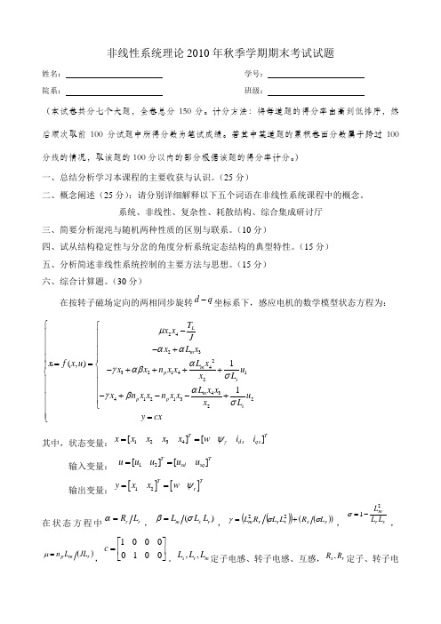
(30分)在按转子磁场定向的两相同步旋转d q -坐标系下,感应电机的数学模型状态方程为:2423243214124341213221(,)1L m m p sm p p s T x x Jx L x L x xf x u x x n x x u x L L x x x n x x n x x u x L y cx μαααγαβσαγβσ⎧⎧-⎪⎪⎪⎪-+⎪⎪⎪⎪==⎪⎨-++++⎨⎪⎪⎪⎪⎪-+--+⎪⎪⎩⎪⎪=⎩其中,状态变量:1234[][]TTd s q s x x x x x wi i γψ==输入变量: 12[][]TTsdsq u u u u u ==输出变量:[][]12TTr y x x wψ==在状态方程中r rR L α=,()m s r L L L βσ=,()()()()s srs rm L RL LR L σσγ+=22,sr m L L L 21-=σ,)r mp JL L n =μ,1000010c ⎡⎤=⎢⎥⎣⎦。
,,s r m L L L 定子电感、转子电感、互感,rs R R ,定子、转子电阻,pn 转子极对数,r ψ转子磁通幅值,qsds i i ,两相同步旋转坐标系d 、q 轴定子电流,qsds u u ,两相同步旋转坐标系d 、q 轴定子电压,w 机械角速度。
具连续分布滞量的偶数阶中立型阻尼偏微分方程解的振动准则
文考虑具有 阻 尼项 和 连续 分 布滞 量 的偶 数 阶 中立 型偏微分方程 :
1 n
h
[(, +∑ ) + xt ) ()(,()]
—
,+∞
J‘ 0
一
J‘ O
( 3 ep 一I()sd = ∞; H )I x( sd)t + b
第1 期
蔡江涛等 :具连续 分布滞 量的偶 数阶中立型阻尼偏微分 方程解 的振动准则
具 中
数 日=日(,) 于 函数 类 , t 属 记 ∈ , 如果 日∈
( 2 ( t 0 ∈a B ) , ): ,
c D, )满 足 日(,)=0 H(,) ( R+ , tf , ts ≠0对 t 5 >≥ t, 。并且在 D上有偏导数 O  ̄ r H O 使 得 H o 和O / s
(2 P() ( +R ) ∑P( M ) t ∈C R , + , f )<1 ,
收稿 日期 :0 8— 6—2 20 0 4
基金项 目: 湖南省 自然科学基金 (6J0 1 和湖南省教育厅科研基金 (6 19 资助项 目 0 J50 ) 0 C8 ) 作者简介 : 蔡江涛 (9 3 )男 , 17 一 , 讲师 , 主要从事微分方程振动理论研究
关键词 : 中立型 ; 连续分布滞量 ; 偏微分方程 ; 振动性
中图分类号 : 15 4 0 7 . 文献标志码 : A 文章编号 :0 1— 35 2 l ) l一 00— 5 10 89 (oo o 0 5 0
d |1 .99j i n 10 — 3 52 1. 10 1 o:03 6/.s .0 1 8 9 .00 O . 1 s
21 00年 1月
带时变时滞的不确定离散奇异系统鲁棒稳定性分析

收稿 日期 : 0 20 —6 作者简 介:翁发禄( 98 )男 , 2 1 -61 . 17 一 , 博士生 ; 毛维杰( 联系人)男 , , 博士 , 教授 , 博士生导师 , j o i .j.d .a w ma@ic z eu c . p u 基金项 目:国家 自然科学基金资助项 目( 17 0 5 6 7 16 ) 60 4 4 , 0 20 2 . 引文格式 :翁发禄 , 毛维杰 带时变时滞 的不确定离 散奇异 系统鲁棒稳 定性分 析 [ ] 东南大学 学报 : J. 自然科学 版 ,0 2,2( 1 :2—9 21 4 S )9 7
摘 要 :为 了降低 不确定 离散 奇异 时变 时滞 系统 稳定 性条 件 的保 守性 , 先 , 首 采用 时滞分 割方 法 , 获 得 了新 的时滞 系统描述 方 法 , 并通 过 综 合考 虑 各 时滞分 割子 区 间, 出 了分 割子 区间依 赖 型 提
L au o y p n v函数 .其 次 , 用 时滞依赖 线性 矩 阵不 等 式技 术 ,将研 究结 果描 述 成 易 于求 解 的严 格 采 线性矩 阵不 等式形 式.通过 Ma a t b工具 箱求解 线 性 矩 阵不 等 式 , l 即可 获得 标 称 系统 正 则 、因果
条件 比时滞 依赖 型条 件具有 更 大 的保 守性 .
奇异 系统 , 又称 为描述 系统 、 隐式 系统 、 广义 状 态空 间系统 、 分 代数 系 统 及 半状 态 系 统 , 泛 存 差 广 在 于许多 实际 系统 中 , 如 工 程领 域 系统 , 会 经 例 社
的成果 大致 可 以分 为两 类 : 时滞 不依 赖 型条 件
Absr c t a t:I r e o d c e s he c ns r a im ft e sa l y c ndto o n e ti ic ee sn n 0 d rt e r a e t o e v ts o tbi t o i nsf ru c ran d s r t i . h i i g l rs t m swi n e a i e v r i g d ly,a d l y p ri o n e h i u se p o e o o t i u a yse t i tr ltm — a y n e a h v ea a tt nig tc n q e i m l y d t b a n a i n w e c p i n o e sn ulrs se r t n e s b n e v ld pe d n a u v f ci n li e d s r to ft ig a y t m f s ,a d a n w u i tr a - e n e tLy p no un to a s i h i c n tu t d i o p e e i e c nsd r t n o l s b n e a s Th n. b s d o e d l y d p n e t o sr ce n c m r h nsv o i e ai fa 1 u i tr l. o v e a e n t ea . e e d n h
合肥工业大学 信号与系统试卷2010
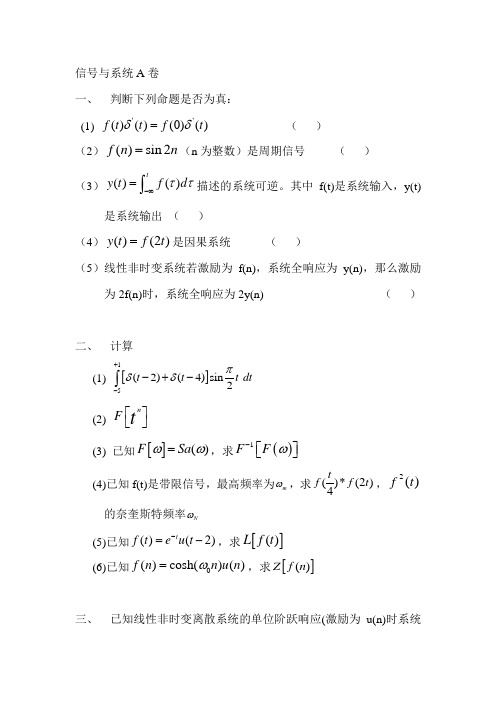
信号与系统A 卷一、 判断下列命题是否为真:(1) ''()()(0)()f t t f t δδ= ( )(2)()sin 2f n n =(n 为整数)是周期信号 ( )(3)()()ty t f d ττ-∞=⎰描述的系统可逆。
其中f(t)是系统输入,y(t)是系统输出 ( )(4)()(2)y t f t =是因果系统 ( )(5)线性非时变系统若激励为f(n),系统全响应为y(n),那么激励为2f(n)时,系统全响应为2y(n) ( )二、 计算(1) []15(2)(4)sin2t t t dt πδδ+--+-⎰(2) n F t ⎡⎤⎣⎦(3) 已知[]()F Sa ωω=,求()1F F ω-⎡⎤⎣⎦(4)已知f(t)是带限信号,最高频率为m ω,求()*(2)4t f f t ,2()f t的奈奎斯特频率N ω(5)已知()(2)t f t e u t -=-,求[]()L f t (6)已知0()cosh()()f n n u n ω=,求[]()Z f n三、 已知线性非时变离散系统的单位阶跃响应(激励为u(n)时系统的零状态响应),1()()2ng n u n ⎛⎫= ⎪⎝⎭,求该系统的单位冲激响应。
四、 绘出下列系统的仿真框图 (1)21002()()()()d y t dy t a a y t b f t dt dt ++= (2) ()3(1)2(2)()y n y n y n f n --+-=五、 如图所示系统()jnt n f t e +∞=-∞=∑,4,|| 1.5/()0j rad s H e πωωω-⎧<⎪⎪=⎨⎪⎪⎩试画出A 、B 、C 三点的频谱(傅里叶变换),并求出信号y(t)。
六、 电路如图所示,激励i(t),响应为电感上电流i1(t),(1) 试求转移函数1()()()zs s H s I s I =,并判断系统的稳定性; (2) 用矢量图方法分析该系统的频响特性,画出频响特性曲线。
数学英语词汇
圆锥面cone顶点vertex旋转单叶双曲面revolution hyperboloids of one sheet旋转双叶双曲面revolution hyperboloids of two sheets柱面cylindrical surface ,cylinder圆柱面cylindrical surface准线directrix抛物柱面parabolic cylinder二次曲面quadric surface椭圆锥面dlliptic cone椭球面ellipsoid单叶双曲面hyperboloid of one sheet双叶双曲面hyperboloid of two sheets旋转椭球面ellipsoid of revolution椭圆抛物面elliptic paraboloid旋转抛物面paraboloid of revolution双曲抛物面hyperbolic paraboloid马鞍面saddle surface椭圆柱面elliptic cylinder双曲柱面hyperbolic cylinder抛物柱面parabolic cylinder空间曲线space curve空间曲线的一般方程general form equations of a space curve空间曲线的参数方程parametric equations of a space curve螺转线spiral螺矩pitch投影柱面projecting cylinder投影projection平面的点法式方程pointnorm form eqyation of a plane法向量normal vector平面的一般方程general form equation of a plane两平面的夹角angle between two planes点到平面的距离distance from a point to a plane空间直线的一般方程general equation of a line in space方向向量direction vector直线的点向式方程pointdirection form equations of a line方向数direction number直线的参数方程parametric equations of a line两直线的夹角anglebetween two lines垂直perpendicular直线与平面的夹角angle between a line and a planes平面束pencil of planes平面束的方程equation of a pencil of planes行列式determinant系数行列式coefficient determinant第八章多元函数微分法及其应用Chapter8 Differentiation of Functions of Severa l Variables and Its Application一元函数function of one variable多元函数function of several variables内点interior point外点exterior point边界点frontier point,boundary point聚点point of accumulation开集openset闭集closed set连通集connected set开区域open region闭区域closed region有界集bounded set无界集unbounded setn维空间n-dimentional space二重极限double limit多元函数的连续性continuity of function of seveal连续函数continuous function不连续点discontinuity point一致连续uniformly continuous偏导数partial derivative对自变量x的偏导数partial derivative with respect to independent variable x高阶偏导数partial derivative of higher order二阶偏导数second order partial derivative混合偏导数hybrid partial derivative全微分total differential偏增量oartial increment偏微分partial differential全增量total increment可微分differentiable必要条件necessary condition充分条件sufficient condition叠加原理superpostition principle全导数total derivative中间变量intermediate variable隐函数存在定理theorem of the existence of implicit function曲线的切向量tangent vector of a curve法平面normal plane向量方程vector equation向量值函数vector-valued function切平面tangent plane法线normal line方向导数directional derivative梯度gradient数量场scalar field梯度场gradient field向量场vector field势场potential field引力场gravitational field引力势gravitational potential曲面在一点的切平面tangent plane to a surface at a point曲线在一点的法线normal line to a surface at a point无条件极值unconditional extreme values条件极值conditional extreme values拉格朗日乘数法Lagrange multiplier method拉格朗日乘子Lagrange multiplier经验公式empirical formula最小二乘法method of least squares均方误差mean square error第九章重积分Chapter9 Multiple Integrals二重积分double integral可加性additivity累次积分iterated integral体积元素volume element三重积分triple integral直角坐标系中的体积元素volume element in rectangular coordinate system柱面坐标cylindrical coordinates柱面坐标系中的体积元素volume element in cylindrical coordinate system球面坐标spherical coordinates球面坐标系中的体积元素volume element in spherical coordinate system反常二重积分improper double integral曲面的面积area of a surface质心centre of mass静矩static moment密度density形心centroid转动惯量moment of inertia参变量parametric variable第十章曲线积分与曲面积分Chapter10 Line(Curve)Integrals and Surface Integrals对弧长的曲线积分line integrals with respect to arc hength第一类曲线积分line integrals of the first type对坐标的曲线积分line integrals with respect to x,y,and z第二类曲线积分line integrals of the second type有向曲线弧directed arc单连通区域simple connected region复连通区域complex connected region格林公式Green formula第一类曲面积分surface integrals of the first type对面的曲面积分surface integrals with respect to area有向曲面directed surface对坐标的曲面积分surface integrals with respect to coordinate elements第二类曲面积分surface integrals of the second type有向曲面元element of directed surface高斯公式gauss formula拉普拉斯算子Laplace operator格林第一公式Green’s first formula通量flux散度divergence斯托克斯公式Stokes formula环流量circulation旋度rotation,curl第十一章无穷级数Chapter11 Infinite Series一般项general term部分和partial sum余项remainder term等比级数geometric series几何级数geometric series公比common ratio调和级数harmonic series柯西收敛准则Cauchy convergence criteria, Cauchy criteria for convergence正项级数series of positive terms达朗贝尔判别法D’Alembert test柯西判别法Cauchy test交错级数alternating series绝对收敛absolutely convergent条件收敛conditionally convergent柯西乘积Cauchy product函数项级数series of functions发散点point of divergence收敛点point of convergence收敛域convergence domain和函数sum function幂级数power series幂级数的系数coeffcients of power series阿贝尔定理Abel Theorem收敛半径radius of convergence收敛区间interval of convergence泰勒级数Taylor series麦克劳林级数Maclaurin series二项展开式binomial expansion近似计算approximate calculation舍入误差round-off error,rounding error欧拉公式Euler’s formula魏尔斯特拉丝判别法Weierstrass test三角级数trigonometric series振幅amplitude角频率angular frequency初相initial phase矩形波square wave谐波分析harmonic analysis直流分量direct component基波fundamental wave二次谐波second harmonic三角函数系trigonometric function system傅立叶系数Fourier coefficient傅立叶级数Forrier series周期延拓periodic prolongation正弦级数sine series余弦级数cosine series奇延拓odd prolongation偶延拓even prolongation傅立叶级数的复数形式complex form of Fourier series第十二章微分方程Chapter12 Differential Equation解微分方程solve a dirrerential equation常微分方程ordinary differential equation偏微分方程partial differential equation,PDE微分方程的阶order of a differential equation微分方程的解solution of a differential equation微分方程的通解general solution of a differential equation初始条件initial condition微分方程的特解particular solution of a differential equation初值问题initial value problem微分方程的积分曲线integral curve of a differential equation可分离变量的微分方程variable separable differential equation隐式解implicit solution隐式通解inplicit general solution衰变系数decay coefficient衰变decay齐次方程homogeneous equation一阶线性方程linear differential equation of first order非齐次non-homogeneous齐次线性方程homogeneous linear equation非齐次线性方程non-homogeneous linear equation常数变易法method of variation of constant暂态电流transient stata current稳态电流steady state current伯努利方程Bernoulli equation全微分方程total differential equation积分因子integrating factor高阶微分方程differential equation of higher order悬链线catenary高阶线性微分方程linera differential equation of higher order自由振动的微分方程differential equation of free vibration强迫振动的微分方程differential equation of forced oscillation串联电路的振荡方程oscillation equation of series circuit二阶线性微分方程second order linera differential equation线性相关linearly dependence线性无关linearly independce二阶常系数齐次线性微分方程second order homogeneour lineardifferential equation withconstant coefficient二阶变系数齐次线性微分方程second order homogeneous linear differential equation with variable coefficient特征方程characteristic equation无阻尼自由振动的微分方程differential equation of free vibration with zero damping固有频率natural frequency简谐振动simple harmonic oscillation,simple harmonic vibration微分算子differential operator待定系数法method of undetermined coefficient共振现象resonance phenomenon欧拉方程Euler equation幂级数解法power series solution数值解法numerial solution勒让德方程Legendre equation微分方程组system of differential equations常系数线性微分方程组system of linera differential equations with constant coefficient。
2010-基于Karush_Kuhn_Tucker最优条件的电网可疑参数辨识与估计
第34卷第1期电网技术V ol. 34 No. 1 2010年1月Power System Technology Jan. 2010 文章编号:1000-3673(2010)01-0056-06 中图分类号:TM 734 文献标志码:A 学科代码:470·4051基于Karush-Kuhn-Tucker最优条件的电网可疑参数辨识与估计曾兵,吴文传,张伯明(电力系统及发电设备控制和仿真国家重点实验室(清华大学电机工程与应用电子技术系),北京市海淀区 100084)A Method to Identify and Estimate Network Parameter Errors Based onKarush-Kuhn-Tucker ConditionZENG Bing, WU Wen-chuan, ZHANG Bo-ming(State Key Laboratory of Control and Simulation of Power Systems and Generation Equipment (Department of Electrical Engineering, Tsinghua University), Haidian District, Beijing 100084, China)ABSTRACT: Network parameter errors may strongly deteriorate the accuracy of state estimation results and affect both reliability and accuracy of other applications, thus state estimation program should possess the function to recognize and estimate element parameters. In this paper, firstly, based on Lagrangian algorithm an iterative method to identify incorrect parameters is proposed to generate branch parameter set to be modified; then a parameter estimation method based on the sensitivity of parameter to objective function, which represents how the parameters affect the quality of the state estimation solution, is researched, and for the chosen distrustful branch this method calculate the sensitivity of parameters of distrustful branch to objective function of state estimation; finally, the variable step-size successive approximation method is used to estimate the parameters of distrustful branch. This method eschews the numerical stability in traditional methods, so it is practicable. The results of IEEE 14-bus system and IEEE 30-bus systems show that the proposed method is corrective.KEY WORDS: network parameter errors identification; network parameter estimation; Karush-Kuhn-Tucker (KKT) condition摘要:电网元件参数的误差会导致能量管理系统的状态估计结果不准确,从而影响其他应用结果的可靠性和精确性,因此状态估计程序应当具有辨识和估计元件参数的功能。
复杂网络
Home Search Collections Journals About Contact us My IOPscienceMapping Koch curves into scale-free small-world networksThis article has been downloaded from IOPscience. Please scroll down to see the full text article.2010 J. Phys. A: Math. Theor. 43 395101(/1751-8121/43/39/395101)View the table of contents for this issue, or go to the journal homepage for moreDownload details:IP Address: 219.220.208.31The article was downloaded on 21/10/2010 at 07:26Please note that terms and conditions apply.IOP P UBLISHING J OURNAL OF P HYSICS A:M ATHEMATICAL AND T HEORETICAL J.Phys.A:Math.Theor.43(2010)395101(16pp)doi:10.1088/1751-8113/43/39/395101Mapping Koch curves into scale-free small-world networksZhongzhi Zhang1,2,Shuyang Gao1,2,Lichao Chen3,Shuigeng Zhou1,2,Hongjuan Zhang2,4and Jihong Guan51School of Computer Science,Fudan University,Shanghai200433,People’s Republic of China2Shanghai Key Lab of Intelligent Information Processing,Fudan University,Shanghai200433,People’s Republic of China3Electrical Engineering Department,University of California,Los Angeles,CA90024,USA4Department of Mathematics,College of Science,Shanghai University,Shanghai200444,People’s Republic of China5Department of Computer Science and Technology,Tongji University,4800Cao’an Road,Shanghai201804,People’s Republic of ChinaE-mail:zhangzz@,sgzhou@ and jhguan@Received8June2010,infinal form7July2010Published1September2010Online at /JPhysA/43/395101AbstractThe class of Koch fractals is one of the most interesting families of fractals,andthe study of complex networks is a central issue in the scientific community.In this paper,inspired by the famous Koch fractals,we propose a mappingtechnique converting Koch fractals into a family of deterministic networkscalled Koch networks.This novel class of networks incorporates somekey properties characterizing a majority of real-life networked systems—apower-law distribution with exponent in the range between2and3,a highclustering coefficient,a small diameter and average path length and degreecorrelations.Besides,we enumerate the exact numbers of spanning trees,spanning forests and connected spanning subgraphs in the networks.All thesefeatures are obtained exactly according to the proposed generation algorithm ofthe networks considered.The network representation approach could be usedto investigate the complexity of some real-world systems from the perspectiveof complex networks.PACS numbers:89.75.Hc,05.10.−a,89.75.Fb,61.43.Hv(Somefigures in this article are in colour only in the electronic version)1.IntroductionThe past decade has witnessed a great deal of activity devoted to complex networks by the scientific community,since many systems in the real world can be described and characterized 1751-8113/10/395101+16$30.00©2010IOP Publishing Ltd Printed in the UK&the USA1by complex networks[1–4].Prompted by the computerization of data acquisition and the increased computing power of computers,researchers have done a lot of empirical studies on diverse real networked systems,unveiling the presence of some generic properties of various natural and manmade networks:power-law degree distribution P(k)∼k−γwith the characteristic exponentγin the range between2and3[5],small-world effect including a large clustering coefficient and small average distance[6],and degree correlations[7,8].The empirical studies have inspired researchers to construct network models with the aim to reproduce or explain the striking common features of real-life systems[1,2].In addition to the seminal Watts–Strogatz’s(WS)small-world network model[6]and Barab´a si–Albert’s (BA)scale-free network model[5],a considerable number of models and mechanisms have been developed to mimic real-world systems,including initial attractiveness[9],aging and cost[10],fitness model[11],duplication[12],weight or traffic driven evolution[13,14], geographical constraint[15],accelerating growth[16,17],coevolution[18]and visibility graph[19],to list a few.Although significant progress has been made in thefield of network modeling and has led to a significant improvement in our understanding of complex systems,it is still a fundamental task and of current interest to construct models mimicking real networks and reproducing their generic properties from different angles[20].In this paper,enlightened by the famous class of Koch fractals,we propose a family of deterministic mathematical networks,called Koch networks,which integrates the observed properties of real networks in a single framework.We derive analytically exact scaling laws for degree distribution,clustering coefficient,diameter,average distance or average path length (APL),degree correlations,even for spanning trees,spanning forests and connected spanning subgraphs.The obtained precise results show that Koch networks have rich topological features:they obey a power-law degree distribution with the exponent lies between2and3; they have a large clustering coefficient and their diameter and APL grow logarithmically with the total number of nodes;and they may be either disassortative or uncorrelated.This work unfolds an alternative perspective in the study of complex networks.Instead of searching generation mechanisms for real networks,we explore deterministic mathematical networks that exhibit some typical properties of real-world systems.As the classical Koch fractals are important for the understanding of geometrical fractals in real systems[21],we believe that Koch networks could provide valuable insights into real-world systems.work constructionIn order to define the networks,wefirst introduce a classical fractal—Koch curve,which was proposed by von Koch[22].The Koch curve,denoted as S1(t)after t generations,can be constructed in a recursive way.To produce this well-known fractal,we begin with an equilateral triangle and let this initial configuration be S1(0).In thefirst generation,we perform the following operations:firstly,we trisect each side of the initial equilateral triangle; secondly,on the middle segment of each side,we construct new equilateral triangles whose interiors lie external to the region enclosed by the base triangle;thirdly,we remove the three middle segments of the base triangle,upon which new triangles were established.Thus,we get S1(1).In the second generation,for each line segment in S1(1),we repeat the above procedure of three operations to obtain S1(2).This process is then repeated for successive generations. As t tends to infinite,the Koch curve is obtained,and its Hausdorff dimension is d f=2ln2ln3 [23].Figure1depicts the structure of S1(2).The Koch curve can be easily generalized to other dimensions by introducing a parameter m(a positive integer)[23,24].The generalization after t generations is denoted by S m(t),which is constructed as follows[23]:start with an equilateral triangle as the initial configuration 2Figure1.Thefirst two generations of the construction for the Koch curve.S m(0).In thefirst generation,we perform the following operations similar to those described in the last paragraph:partition each side of the initial triangle into2m+1segments,which are consecutively numbered1,2,...,2m,2m+1from one endpoint of the side to the other; construct a new small equilateral triangle on each even-numbered segment so that the interiors of the new triangles lie in the exterior of the base triangle;remove the segments upon which triangles were constructed.In this way we obtain S m(1).Analogously,we can get S m(t) from S m(t−1)by repeating recursively the procedure of the above three operations for each existing line segment in generation t−1.In the infinite t limit,the Hausdorff dimension ofthe generalized Koch curves d f=ln(4m+1)ln(2m+1)[23].Figure2shows the structure of S2(2).The generalized Koch curves can be used as a basis of a new class of networks: sides(excluding those deleted)of the triangles of the Koch curves constructed at arbitrary generations are mapped to nodes,which are connected to one another if their corresponding sides in the Koch curves are in contact.For uniformity,the three sides of the initial equilateral triangle of S m(0)also correspond to three different nodes.We shall call the resultant networks Koch networks.Note that after establishing each side of a triangle constructed at a given generation of the Koch curves,although some segments of it will be removed at subsequent steps,we look at its remaining segments as a whole and map it to only one node.Figures3 and4show two networks corresponding to S1(2)and S2(2),respectively.Obviously,Koch networks have an infinite number of nodes.But in what follows we shall generally consider the network characteristics after afinite number of generations in the development of complete Koch networks.From our analytical results,we can quickly obtain the characteristics of the complete networks by taking the limit of large t.However,the numerical results are necessarily limited to networks withfinite order(number of all nodes).3.Generation algorithmAccording to the construction process of the generalized Koch curves and the proposed method of mapping from Koch curves to Koch networks,we can introduce an iterative algorithm with3Figure2.Thefirst two generations of the construction for the generalized Koch curve in the caseof m=2.Figure3.The network derived from S1(2).ease to create Koch networks,denoted by K m,t after t generation evolutions.The algorithm is as follows:initially(t=0),K m,0consists of three nodes forming a triangle.For t 1, K m,t is obtained from K m,t−1by adding m groups of nodes for each of the three nodes of every existing triangle in K m,t−1.Each node group has two nodes.These two new nodes and their‘mother’nodes are linked to one another shaping a new triangle.In other words,to obtain K m,t from K m,t−1,we replace each of the existing triangles of K m,t−1by the connected clusters on the rightmost side offigure5.Figures3and4illustrate the growing process of the networks for two particular cases of m=1and m=2,respectively.Note that in the peculiar case of m=1,the networks under consideration reduce to the one previously studied in[25].Let us compute the order and size(number of all edges)of the Koch networks K m,t.To this end,wefirst consider the total number of triangles L (t)that exist at step t.By construction 4Figure4.The network corresponding to S2(2).Figure5.Iterative construction method for the Koch networks.(seefigure5),this quantity increases by a factor of3m+1,i.e.L (t)=(3m+1)L (t−1). Considering L (0)=1,we have L (t)=(3m+1)t.Denote L v(t)and L e(t)as the numbers of nodes and edges created at step t,respectively.Note that each triangle in K m,t−1 will give rise to6m new nodes and9m new edges at step t;then one can easily obtain L v(t)=6m L (t−1)=6m(3m+1)t−1and L e(t)=9m L (t−1)=9m(3m+1)t−1,both of which hold for arbitrary t>0.Then,the total numbers of nodes N t and edges E t present at step t areN t=tt i=0L v(t i)=2(3m+1)t+1(1)andE t=tt i=0L e(t i)=3(3m+1)t,(2)respectively.Thus,the average degree isk =2E tN t =6(3m+1)t2(3m+1)t+1,(3)5which is approximately3for large t,showing that Koch networks are sparse as most real-life networks[1–4].4.Topological propertiesNow we study some relevant characteristics of the Koch networks K m,t,focusing on degree distribution,clustering coefficient,diameter,average distance,degree correlations,spanning trees,spanning forests and connected spanning subgraphs.We emphasize that this is the first analytical study for counting spanning trees,spanning forests and connected spanning subgraphs in scale-free networks.4.1.Degree distributionLet k i(t)be the degree of node i at time t.When node i enters the network at step t i(t i 0), it has a degree of2,namely k i(t i)=2.To determine k i(t),wefirst consider the number of triangles involving node i at step t that is denoted by L (i,t).These triangles will give rise to new nodes linked to node i at step t+1.Then at step t i,L (i,t i)=1.By construction, for any triangle involving node i at a given step,it will lead to m new triangles passing by node i at a next step.Thus,L (i,t)=(m+1)L (i,t−1).Considering the initial condition L (i,t i)=1,we have L (i,t)=(m+1)t−t i.On the other hand,each triangle passing by node i contains two links connected to i;therefore,we have k i(t)=2L (i,t).Then we obtaink i(t)=2L (i,t)=2(m+1)t−t i.(4) In this way,at time t the degree of the arbitrary node i of Koch networks has been computed explicitly.From equation(4),it is easy to see that at each step the degree of a node increases m times,i.e.k i(t)=(m+1)k i(t−1).(5) Equation(4)shows that the degree spectrum of Koch networks is discrete.Thus,we can get the degree distribution P(k)of the Koch networks via the cumulative degree distribution [3]given byP cum(k)=1N tτ t iL v(τ)=2×(3m+1)t i+12×(3m+1)+1.(6)Substituting t i=t−ln(k2)ln(m+1)in this expression givesP cum(k)=2×(3m+1)t×k2−ln(3m+1)ln(m+1)+12×(3m+1)t+1.(7)In the infinite t limit,we obtainP cum(k)=2ln(3m+1)ln(m+1)×k−ln(3m+1)ln(m+1).(8) So the degree distribution follows a power-law form P(k)∼k−γwith the exponentγ=1+ln(3m+1)ln(m+1)belonging to the interval[2,3].When m increases from1to infinite,γdecreases from3to2.It should be stressed that the exponent of degree distribution of most real scale-free networks also lies in the same range between2and3.6Figure6.Semilogarithmic plot of the average clustering coefficient C t versus the networkorder N t.4.2.Clustering coefficientBy definition,the clustering coefficient[6]of a node i with degree k i is the ratio between thenumber of triangles e i that actually exist among the k i neighbors of node i and the maximumpossible number of triangles involving i,k i(k i−1)/2,namely C i=2e i/[k i(k i−1)].For Koch networks,we can obtain the exact expression of the clustering coefficient C(k)for asingle node with degree k.By construction,for any given node having a degree k,there are juste=k2triangles connected with this node;see also equation(4).Hence there is a one-to-onecorresponding relation between the clustering coefficient of a node and its degree:for a node of degree k,C(k)=1k−1,(9)which shows a power-law scaling C(k)∼k−1in the large limit of k,in agreement with the behavior observed in a variety of real-life systems[26].After t step growth,the average clustering coefficient C t of the whole network K m,t, defined as the mean of Cis over all nodes in the network,is given byC t=1N ttr=01G r−1×L v(r),(10)where the sum runs over all the nodes of all generations and G r is the degree of those nodes created at step r,which is given by equation(4).In the limit of large N t,equation(10) converges to a nonzero value C,as reported infigure6.For m=1,2and3,C is0.82008, 0.88271and0.91316,respectively.As m approaches infinite,C converges to1.Thus,C increases with m:when m grows from1to infinite,C increases form0.82008to1.Therefore, for the full range of m,the the average clustering coefficient of Koch networks is very high.74.3.DiameterMost real networks are small-world,i.e.their average distance grows logarithmically with network order or slower.Here the average distance means the minimum number of edges connecting a pair of nodes,averaged over all node pairs.For a general network,it is not easy to derive a closed formula for its average distance.However,the whole family of Koch networks has a self-similar structure,allowing for analytically calculating the average distance,which approximately increases as a logarithmic function of the network order.We leave the detailed exact derivation about the average distance to the next subsection.Here we provide the exact result of the diameter of K m,t denoted by Diam(K m,t)for all parameters m,which is defined as the maximum of the shortest distances between all pairs of nodes.Small diameter is consistent with the concept of small-world.The obtained diameter also scales logarithmically with the network order.The computation details are presented as follows.Clearly,at step t=0,Diam(K m,0)is equal to1.At each step t 1,we call newly created nodes at this step as active nodes.Since all active nodes are attached to those nodes existing in K m,t−1,so one can easily see that the maximum distance between any active node and those nodes in K m,t−1is not more than Diam(K m,t−1)+1and that the maximum distance between any pair of active nodes is at most Diam(K m,t−1)+2.Thus,at any step,the diameter of the network increases by2at most.Then we get2(t+1)as the diameter of Diam(K m,t). Equation(1)indicates that the logarithm of the order of Diam(K m,t)is proportional to t in the large limit t.Thus the diameter Diam(K m,t)grows logarithmically with the network order, showing that the Koch networks are small-world.4.4.Average path lengthUsing a method similar to but different from those in the literature[27,28],we now study analytically the average path length d t of the Koch networks K m,t.It follows thatd t=D tot(t)N t(N t−1)/2,(11)where D tot(t)is the total distance between all couples of nodes,i.e.D tot(t)=i∈K m,t,j∈K m,t,i=jd ij(t),(12)where d ij(t)is the shortest distance between nodes i and j in the networks K m,t.Note that Koch networks have a self-similar structure,which allows us to address D tot(t) analytically.This self-similar structure is obvious from an equivalent network construction method:to obtain K m,t,one can make3m+1copies of K m,t−1and join them at the hubs (namely nodes with largest degree).As shown infigure7,the network K m,t+1may be obtained by the juxtaposition of3m+1copies of K m,t,which are labeled as K1m,t,K2m,t,...,K3m m,t,andK3m+1m,t ,respectively.We continue by exhibiting the procedure of the determination of the total distance and present the recurrence formula,which allows us to obtain D tot(t+1)of the t+1generation from D tot(t)of the t generation.From the obvious self-similar structure of Koch networks,it is easy to see that the total distance D tot(t+1)satisfies the recursion relationD tot(t+1)=(3m+1)D tot(t)+ t,(13) 8Figure7.Second construction method of Koch networks that highlights self-similarity.Thegraph after t+1construction steps,K m,t+1,consists of3m+1copies of K m,t denoted as Kθm,t(θ=1,2,3,...,3m,3m+1),which are connected to one another as above.where t is the sum over all shortest paths whose endpoints are not in the same Kθm,t branch. The solution of equation(13)isD tot(t)=(3m+1)t−1D tot(1)+t−1τ=1(3m+1)t−τ−1 τ.(14)All the paths contributing to t must go through at least one of the three edge nodes(i.e.the gray nodes X,Y and Z infigure7)at which the different Kθm,t branches are connected.The analytical expression for t,called the length of crossing paths,is found below.Let α,βt be the sum of the lengths of all shortest paths with endpoints in Kαm,t and Kβm,t. Based on whether or not two branches are adjacent,we sort the crossing path length α,βt into two classes:if Kαm,t and Kβm,t meet at an edge node, α,βt rules out the paths where either endpoint is that shared edge node.For example,each path contributed to 1,2t should not end at node X.If Kαm,t and Kβm,t do not meet, α,βt excludes the paths where either endpoint is any edge node.For instance,each path contributed to 2,m+2tshould not end at node X or Y.We can easily compute that the numbers of the two types of crossing paths are3m2+3m2and3m2,respectively.On the other hand,any two crossing paths belonging to the same class have identical length.Thus,the total sum t is given byt=3m2+3m21,2t+3m2 2,m+2t.(15)In order to determine 1,2t and 2,m+2t,we defines t=i∈K m,t,i=Xd iX(t).(16)Considering the self-similar network structure,we can easily know that at time t+1,the quantity s t+1evolves recursively ass t+1=(m+1)s t+2m[s t+(N t−1)]=(3m+1)s t+4m(3m+1)t.(17)9Using s0=2,we haves t=(4mt+6m+2)(3m+1)t−1.(18) Having obtained s t,the next step is to compute the quantities 1,2t and 2,m+2tgiven by 1,2t=i∈K1m,t,j∈K2m,ti,j=Xd ij(t+1)=i∈K1m,t,j∈K2m,ti,j=X[d iX(t+1)+d jX(t+1)]=(N t−1)i∈K1m,ti=X d iX(t+1)+(N t−1)j∈K2m,tj=Xd jX(t+1)=2(N t−1)i∈K1m,ti=Xd iX(t+1)=2(N t−1)s t,(19) and2,m+2t =i∈K2m,t,i=Xj∈K m+2m,t,j=Yd ij(t+1)=i∈K2m,t,i=Xj∈K m+2m,t,j=Y[d iX(t+1)+d XY(t+1)+d jY(t+1)]=2(N t−1)s t+(N t−1)2,(20)where d XY(t+1)=1has been used.Substituting equations(19)and(20)into equation(15), we obtaint=(9m2+3m)(N t−1)s t+3m2(N t−1)2=12m(2mt+4m+1)(3m+1)2t.(21) Inserting equations(21)for τinto equation(14),and using D tot(1)=48m2+21m+3,we can exactly obtain the expression for D tot(t)asD tot(t)=(3m+1)t−13[3m+5+(24mt+24m+4)(3m+1)t].(22)By inserting equation(22)into equation(11),one can obtain the analytical expression for d t:d t=3m+5+(24mt+24m+4)(3m+1)t3(3m+1)[2(3m+1)t+1],(23)which approximates4mt3m+1in the infinite t,implying that the APL shows a logarithmic scalingwith network order.This again shows that the Koch networks exhibit a small-world behavior. We have checked our analytic result for d t given in equation(23)against numerical calculations for different m and various t.In all the cases we obtain complete agreement between our theoretical formula and the results of numerical investigation,seefigure8.10Figure8.Average path length d t versus network order N t on a semi-log scale.The solid lines areguides to the eyes.4.5.Degree correlationsDegree correlation is a particularly interesting subject in thefield of network science[7,8, 29–32]because it can give rise to some interesting network structure effects.An interesting quantity related to degree correlations is the average degree of the nearest neighbors for nodes with degree k,denoted as k nn(k),which is a function of the node degree k[30,31].When k nn(k)increases with k,it means that nodes have a tendency to connect to the nodes with a similar or larger degree.In this case the network is defined as assortative[7,8].In contrast, if k nn(k)is decreasing with k,which implies that the nodes of large degree are likely to have near neighbors with small degree,then the network is said to be disassortative.If correlations are absent,k nn(k)=const.We can exactly calculate k nn(k)for Koch networks using equations(4)and(5)to work out how many links are made at a particular step to nodes with a particular degree.By construction,we have the following expression:k nn(k)=1L v(t i)k(t i,t)ti=t i−1ti=0m L v(t i)k(t i,t i−1)k(t i,t)+ti=tti=t i+1m L v(t i)k(t i,t i−1)k(t i,t)+1(24)for k=2(m+1)t−t i.Here thefirst sum on the right-hand side accounts for the links made tonodes with a larger degree(i.e.ti <t i)when the node was generated at t i.The second sumdescribes the links made to the current smallest degree nodes at each step ti >t i.The last term1accounts for the link connected to the simultaneously emerging node.In order to compute equation(24),we distinguish two cases according to the parameter m:m=1and m 2.When m=1,we havek nn(k)=t+2.(25)11Thus,in the case of m=1,the networks show the absence of correlations in the full range of t.From equations(25)and(1)we can easily see that for large t,k nn(k)is approximately a logarithmic function of the network order N t,namely k nn(k)∼ln N t,exhibiting a similar behavior as that of the BA model[31]and the two-dimensional random Apollonian network [32].When m 2,equation(24)is simplified tok nn(k)=3m+1)m−1(m+1)23m+1t i−m+3m−1+2mm+1(t−t i).(26)Thus after the initial step k nn(k)grows linearly with time.Writing equation(26)in terms of k,it is straightforward to obtaink nn(k)=3m+1m−1(m+1)23m+1tk2−ln[(m+1)23m+1]ln(m+1)−m+3m−1+2mm+1lnk2ln(m+1).(27)Therefore,k nn(k)is approximately a power-law function of k with negative exponent,which shows that the networks are disassortative.Note that k nn(k)of the Internet exhibits a similar power-law dependence on the degree k nn(k)∼k−ω,withω=0.5[30].4.6.Spanning trees,spanning forests and connected spanning subgraphsSpanning trees,spanning forests and connected spanning subgraphs are important quantities of networks,and the enumeration of these interesting quantities in networks is a fundamental issue[33–37].However,explicitly determining the numbers of these quantities in networks is a theoretical challenge[38].Fortunately,the peculiar construction of Koch networks makes it possible to derive exactly the three variables.4.6.1.Spanning trees.By definition,a spanning tree of any connected network is a minimal set of edges that connect every node.The problem of spanning trees is closely related to various aspects of networks,such as reliability[39,40],optimal synchronization[41]and random walks[42].Thus,it is of great interest to determine the exact number of spanning trees[43].In what follows we will examine the number of spanning trees in Koch networks.Note that in the Koch networks K m,t there are L (t)=(3m+1)t triangles,but there are no cycles of length more than3.For each of L (t)=(3m+1)t triangles,to assure that its three nodes are in one tree,only two edges of it must be present.Obviously,there are three possibilities for this.Thus,the total number of spanning trees in K m,t,denoted by N ST(t),isN ST(t)=3L (t)=3(3m+1)t.(28) We proceed to represent N ST(t)as a function of the network order N t,with the aim to provide the relation governing the two quantities.From equation(1),we have(3m+1)t=N t−12. This expression allows one to write N ST(t)in terms of N t asN ST(t)=3(N t−1)/2.(29)Thus,the number of spanning trees in K m,t increases exponentially with the network order N t,which means that there exists a constant E ST,called as the entropy of spanning trees, describing this exponential growth[34]:E ST=limN t→∞ln N ST(t)N t=12ln3.(30)In addition to the above analytical computation,according to the previously known result [44],one can also obtain numerically but exactly the number of spanning trees,N ST(t),by 12computing the nonzero eigenvalues of the Laplacian matrix associated with the networks K m,t asN ST(t)=1N ti=N t−1i=1λi(t),(31)whereλi(t)(i=1,2,...,N t−1)are the N t−1nonzero eigenvalues of the Laplacian matrix, denoted by L t,for the networks K m,t,which is defined as follows:its non-diagonal element l ij(t)(i=j)is−1(or0)if nodes i and j are(or not)directly linked to each other,while the diagonal entry l ii(t)is exactly the degree of node i.Using equation(31),we have calculated directly the number of spanning trees in the networks K m,t,and the results from equation(31)are fully consistent with those obtained from equation(28),showing that our analytical formula is right.It should be stressed that although expression(31)seems compact,it is involved in the computation of the eigenvalues of a matrix of order N t×N t,which makes heavy demands on time and computational resources. Thus,it is not acceptable for large networks.In particular,by virtue of the eigenvalue method it is difficult and even impossible to obtain the entropy E ST.Our analytical computation can get around the two difficulties,but is only applicable to peculiar networks.4.6.2.Spanning forests.To define spanning forests,wefirst recall the definition for a spanning subgraph.A spanning subgraph of a network is a subgraph having the same node as of the network but having partial or all edges of the original graph.A spanning forest of a network is a spanning graph of it that is a disjoint union of trees(here an isolated node is consider as a tree),i.e.a spanning graph without any cycle.The enumeration of spanning forests is very interesting since it corresponds to the partition function of the q-state Potts model[45]in the limit of q→0.For a general network,it is very hard to count the number of its spanning subgraphs.But below we will show that for the Koch networks K m,t,the number of spanning subgraphs,N SF(t),can be obtained explicitly.Analogous to the enumeration of spanning trees,for each triangle in K m,t,to guarantee the absence of cycle among its three nodes,at least one edge must be removed.And there are total seven possibilities for deleting the edges of a triangle.Then the number of spanning forests in K m,t isN SF(t)=7L (t)=7(3m+1)t,(32) which can be rewritten as a function of the network order N t asN SF(t)=7(N t−1)/2.(33) Therefore,N SF(t)also grows exponentially in N t,which allows for defining the entropy of the spanning forests of Koch networks as the limiting value[46]:E SF=limN t→∞ln N SF(t)N t=12ln7.(34)Thus,we have obtained the rigorous results for the number of spanning forests in Koch networks and its entropy.4.6.3.Connected spanning subgraphs.As the name suggests,a connected spanning subgraph of a connected network is a spanning subgraph of the network,which remains connected.By applying a method similar to that given above,we can compute the number of connected spanning subgraphs in the Koch networks K m,t,which is denoted by N CSS(t).For any triangle in K m,t,to ensure the connectedness of its three nodes,at most one edge can be13。
【计算机应用】_差分方程_期刊发文热词逐年推荐_20140725
2009年 序号 1 2 3 4
科研热词 鲁棒控制 混合h2/h∞控制 差分进化算法 多面体不确定性
推荐指数 1 1 1 1
2010年 序号 1 2 3 4 5 6 7 8 9 10 11 12 13 14 15
科研热词 推荐指数 收敛性 2 高阶交错网格有限差分法 1 静态场边值问题 1 误差估计 1 等价弹性波动方程 1 稳定性 1 波场分离 1 有限差分法 1 有限体积元方法 1 延迟抛物微分方程 1 完全匹配层吸收边界条件 1 交替方向方法 1 二维粘性波动方程 1 matlab 1 crank-nicolson差分格式 1
2012年 序号 1 2 3 4 5 6 7 8 9 10 11 12 13 14 15 16 17 18 19 20 21 22 23 24 25
科研热词 解的存在唯一性 紧致差分格式 收敛性 有限差分 高精度紧致差分格式 高精度
推荐指数 3 3 3 2 1 1 1 非线性schroedinger方程 1 非线性schr(o)dinger方程 1 非线性 1 紧致交错网格 1 格子波尔兹曼方法 1 广义分布函数 1 对流扩散方程 1 完全匹配层 1 交替方向隐式格式 1 井间地震 1 二维波动方程 1 一维burgers守恒型方程 1 weno差分格式 1 unique solvability 1 tti介质 1 nonlinear schrsdinger equation1 linearized compact difference 1 scheme convergence 1
2013年 序号 1 2 3 4 5 6 7 8 9 10 11 12 13 14 15 16 17 18 19 20 21 22 23
科研热词 推荐指数 阶梯效应 1 能量泛函 1 联合紧致差分格式 1 紧致差分格式 1 稳定性 1 直接法 1 水平集 1 有限差分法 1 显式差分 1 收敛性 1 广义极小剩余法 1 巴黎期权特性 1 定价模型 1 图像去噪 1 图像分割 1 唯一性 1 可转债 1 全变分模型 1 richardson外推 1 helmholtz方程 1 gpu 1 euler-lagrange分裂格式 1 black-scholes方程 1
水力过渡计算
with the of
with, it is accuracy. amount
some of the necessary physical description
at the time of running and need a great
On the other hand, certain
are only known with limited
such a detailed
would be very time-consuming
computer resources. Thus, even though it is possible to develop a computer model representing the system in an exact way, the needs of time and resources would override the objective of accuracy. Some idealizations and simplifications render the problem more manageable, without compromising, in any case, the validity of the results, to neglect from an engineering point of view. In many instances, see [2], it is even acceptable the rigid model or mass oscillation. the elastic effects and use a more simple model,
1. I N T R O D U C T I O N