MATLAB单相机校准程序中文
MATLAB汉化指南
MATLAB汉化指南MATLAB汉化指南作者:junziyang Email:**************一、汉化原理简介MATLAB的界面是用JA V A语言实现的(从6.5版以后),其源文件位于MATLAB安装目录下的java\jar 文件夹中的.jar包中。
为了便于MATLAB的本地化(Localization),MATLAB中的一些字符信息(例如,菜单、提示信息等等)没有直接写到JA V A代码中,而是被分离了出来,保存在一种扩展名为.properties 的文件中。
在.properties文件中,每条信息被赋予了一个键值,通过在JA V A程序中调用这些键值,就可以使用键值对应的字符信息。
因此,如果把键值对应的字符信息翻译成不同的语言,不用修改JA V A代码,就可以改变程序中显示的字符的语言。
JA V A程序运行时会根据计算机的“区域和语言选项”中的设置,来自动选择本地语言。
感兴趣的朋友可以试着在“区域和语言选项”中,将语言和位置分别设置为“日语”和“日本”然后启动MATLAB 看看会有什么变化。
设置方法:“开始”-“控制面板”-“日期、时间、语言和区域设置”-“区域和语言设置”-在区域设置选项卡中,上面的下拉框中选“日语”,下面的选“日本”。
如果不出意外,你会发现你的MATLAB变成日文版的了。
现在可能会有人问了,为什么选“中文”和“中国”时MATLAB不是中文版的呢?原因是.jar包中没有中文对应的.properties文件。
JA V A通过.properties文件名中的语言和国家代码来选择合适的.properties文件,例如:*_ja_JP.properties 对应日文版,*_zh_CN.properties对应中文版,没有语言和国家代码的默认为英文版。
当找不到本地版本时,默认会调用英文版的.properties文件。
由于.jar 包中有日文版的.properties文件,所以上面修改区域和语言设置后MATLAB会变为日文版。
多相机标定 matlab

多相机标定 matlab多相机标定是计算机视觉中的一个重要问题,它涉及到了多个相机的内参和外参的标定。
在Matlab中,你可以使用Computer Vision System Toolbox来进行多相机标定。
这个工具箱提供了一些函数和工具,可以帮助你完成多相机标定的任务。
在进行多相机标定时,首先需要收集一组已知的三维空间点的坐标和它们在各个相机中的投影坐标。
这些点通常是通过在实际场景中放置标定板或者其他已知形状的物体来获取的。
然后,你可以使用Matlab中的`stereocalibrate`函数来进行多相机标定。
这个函数可以根据已知的三维点和它们在相机中的投影坐标来计算出相机的内参和外参。
在使用`stereocalibrate`函数时,你需要将每个相机的内参矩阵、畸变系数以及相机之间的相对姿态作为输入。
这些参数可以通过单独对每个相机进行标定来获得。
一旦完成了多相机标定,你就可以使用`stereoParameters`对象来表示每对相机之间的标定结果,包括相机之间的旋转矩阵和平移向量等信息。
除了`stereocalibrate`函数,Matlab中的Computer VisionSystem Toolbox还提供了其他一些用于多相机标定的函数和工具,比如`extrinsics`函数用于计算相机之间的相对姿态,`stereoCameraCalibrator`应用程序用于交互式地进行多相机标定等。
总之,在Matlab中进行多相机标定需要收集好的标定数据,然后使用Computer Vision System Toolbox中提供的函数和工具来进行标定,最终得到每个相机的内参和外参信息,以及相机之间的相对姿态信息。
这些信息可以帮助你在后续的立体视觉和三维重建任务中准确地进行像素到实际世界坐标的转换,从而实现更精准的计算机视觉应用。
三点标定法 matlab

三点标定法是一种常用的标定相机内部参数和外部参数的方法,可以通过拍摄已知标定板的图像来计算相机的内部参数和外部参数。
在MATLAB 中,可以使用以下步骤进行三点标定法的标定:
1. 准备标定板:选择一个已知尺寸和标定信息的标定板,例如棋盘格标定板。
将标定板放在相机前,使其完全覆盖相机的成像区域。
2. 拍摄标定板图像:使用相机拍摄标定板图像,确保图像清晰、无畸变。
3. 提取标定板特征点:使用特征点检测算法(如SURF、SIFT、ORB 等)从图像中提取标定板的特征点。
4. 计算基础矩阵:使用FindFundamentalMat 函数计算相机和标定板之间的基础矩阵。
5. 计算本质矩阵:使用RANSAC 算法计算相机的本质矩阵。
6. 计算相机参数:使用本质矩阵和基础矩阵计算相机的内部参数和外部参数。
7. 可视化标定结果:将标定结果可视化为相机的内部参数矩阵和外部参数矩阵。
需要注意的是,三点标定法需要拍摄至少三张标定板的图像,以确保标定结果的准确性。
同时,在拍摄图像时需要保持相机的位置和朝向不变,避免因相机位置和朝向的变化导致标定结果不准确。
matlab相机定标工具箱程序的算法原理
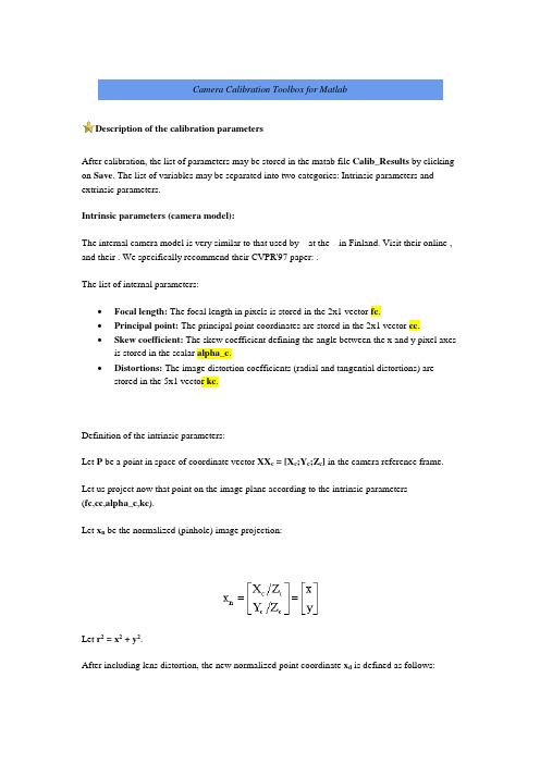
Camera Calibration Toolbox for MatlabDescription of the calibration parametersAfter calibration, the list of parameters may be stored in the matab file Calib_Results by clicking on Save. The list of variables may be separated into two categories: Intrinsic parameters and extrinsic parameters.Intrinsic parameters (camera model):The internal camera model is very similar to that used by at the in Finland. Visit their online , and their . We specifically recommend their CVPR'97 paper: .The list of internal parameters:•Focal length: The focal length in pixels is stored in the 2x1 vector fc.•Principal point: The principal point coordinates are stored in the 2x1 vector cc.•Skew coefficient: The skew coefficient defining the angle between the x and y pixel axes is stored in the scalar alpha_c.•Distortions: The image distortion coefficients (radial and tangential distortions) are stored in the 5x1 vector kc.Definition of the intrinsic parameters:Let P be a point in space of coordinate vector XX c = [X c;Y c;Z c] in the camera reference frame.Let us project now that point on the image plane according to the intrinsic parameters(fc,cc,alpha_c,kc).Let x n be the normalized (pinhole) image projection:Let r2 = x2 + y2.After including lens distortion, the new normalized point coordinate x d is defined as follows:where dx is the tangential distortion vector:Therefore, the 5-vector kc contains both radial and tangential distortion coefficients (observe that the coefficient of 6th order radial distortion term is the fifth entry of the vector kc).It is worth noticing that this distortion model was first introduced by Brown in 1966 and called "Plumb Bob" model (radial polynomial + "thin prism" ). The tangential distortion is due to "decentering", or imperfect centering of the lens components and other manufacturing defects in a compound lens. For more details, refer to Brown's original publications listed in the .Once distortion is applied, the final pixel coordinates x_pixel = [x p;y p] of the projection of P on the image plane is:Therefore, the pixel coordinate vector x_pixel and the normalized (distorted) coordinate vector x d are related to each other through the linear equation:where KK is known as the camera matrix, and defined as follows:In matlab, this matrix is stored in the variable KK after calibration. Observe that fc(1) and fc(2) are the focal distance (a unique value in mm) expressed in units of horizontal and vertical pixels. Both components of the vector fc are usually very similar. The ratio fc(2)/fc(1), often called "aspect ratio", is different from 1 if the pixel in the CCD array are not square. Therefore, the camera model naturally handles non-square pixels. In addition, the coefficient alpha_c encodes the angle between the x and y sensor axes. Consequently, pixels are even allowed to benon-rectangular. Some authors refer to that type of model as "affine distortion" model.In addition to computing estimates for the intrinsic parameters fc, cc, kc and alpha_c, the toolbox also returns estimates of the uncertainties on those parameters. The matlab variables containing those uncertainties are fc_error, cc_error, kc_error, alpha_c_error. For information, those vectors are approximately three times the standard deviations of the errors of estimation.Here is an example of output of the toolbox after optimization:In this case fc = [657.30254 ; 657.74391] and fc_error = [0.28487 ; 0.28937], cc = [302.71656 ; 242.33386], cc_error = [0.59115 ; 0.55710], ...Important Convention: Pixel coordinates are defined such that [0;0] is the center of the upper left pixel of the image. As a result, [nx-1;0] is center of the upper right corner pixel, [0;ny-1] is the center of the lower left corner pixel and [nx-1;ny-1] is the center of the lower right corner pixel where nx and ny are the width and height of the image (for the images of the first example,nx=640 and ny=480). One matlab function provided in the toolbox computes that direct pixel projection map. This function is project_points2.m. This function takes in the 3D coordinates of a set of points in space (in world reference frame or camera reference frame) and the intrinsic camera parameters (fc,cc,kc,alpha_c), and returns the pixel projections of the points on the image plane. See the information given in the function.The inverse mapping:The inverse problem of computing the normalized image projection vector x n from the pixel coordinate x_pixel is very useful in most machine vision applications. However, because of the high degree distortion model, there exists no general algebraic expression for this inverse map (also called normalization). In the toolbox however, a numerical implementation of inverse mapping is provided in the form of a function: normalize.m. Here is the way the function should be called: x n = normalize(x_pixel,fc,cc,kc,alpha_c). In that syntax, x_pixel and x n may consist of more than one point coordinates. For an example of call, see the matlab functioncompute_extrinsic_init.m.Reduced camera models:Currently manufactured cameras do not always justify this very general optical model. For example, it now customary to assume rectangular pixels, and thus assume zero skew (alpha_c=0). It is in fact a default setting of the toolbox (the skew coefficient not being estimated). Furthermore, the very generic (6th order radial + tangential) distortion model is often not considered completely. For standard field of views (non wide-angle cameras), it is often not necessary (and not recommended) to push the radial component of distortion model beyond the 4th order (i.e. keeping kc(5)=0). This is also a default setting of the toolbox. In addition, the tangential component of distortion can often be discarded (justified by the fact that most lenses currently manufactured do not have imperfection in centering). The 4th order symmetric radial distortion with no tangential component (the last three component of kc are set to zero) is actually the distortion model used by . Another very common distortion model for good optical systems or narrow field of view lenses is the second order symmetric radial distortion model. In that model, only the first component of the vector kc is estimated, while the other four are set to zero. This model is also commonly used when a few images are used for calibration (too little data to estimate a more complex model). Aside from distortions and skew, other model reductions are possible. For example, when only a few images are used for calibration (e.g. one, two or three images) the principal point cc is often very difficult to estimate reliably . It is known to be one of the most difficult part of the native perspective projection model to estimate (ignoring lens distortions). If this is the case, it is sometimes better (and recommended) to set the principal point at the center of the image (cc = [(nx-1)/2;(ny-1)/2]) and not estimate it further. Finally, in few rare instances, it may be necessary to reject the aspect ratio fc(2)/fc(1) from the estimation. Although this final model reduction step is possible with the toolbox, it is generally not recommended as the aspect ratio is often 'easy' to estimate very reliably. For more information on how to perform model selection with the toolbox, visit the .Correspondence with Heikkil䧳notation:In the original , the internal parameters appear with slightly different names. The following table gives the correspondence between the two notation schemes:A few comments on Heikkil䧳model:•Skew is not estimated (alpha_c=0). It may not be a problem as most cameras currently manufactured do not have centering imperfections.•The radial component of the distortion model is only up to the 4th order. This is sufficient for most cases.•The four variables (f,Du,Dv,su) replacing the 2x1 focal vector fc are in general impossible to estimate separately. It is only possible if two of those variables are known(for example the metric focal value f and the scale factor su). See for more information.Correspondence with Reg Willson's notation:In his original , uses a different notation for the camera parameters. The following table gives the correspondence between the two notation schemes:Willson uses a first order radial distortion model (with an additional constant kappa1) that does not have an easy closed-form corespondence with our distortion model (encoded with the coefficients kc(1),...,kc(5)). However, we included in the toolbox a function calledwillson_convert that converts the entire set of Willson's parameters into our parameters (including distortion). This function is called in another function willson_read that directly loads in a calibration result file generated by Willson's code and computes the set parameters (intrinsic and extrinsic) following our notation (to use that function, first set the matlab variable calib_file to the name of the original willson calibration file).A few extra comments on Willson's model:•Similarly to Heikkil䧳model, the skew is not included in the model (alpha_c=0).•Similarly to Heikkil䧳model, the four variables (f,sx,dpx,dpy) replacing the 2x1 focal vector fc are in general impossible to estimate separately. It is only possible if two ofthose variables are known (for example the metric focal value f and the scale factor sx).Extrinsic parameters:•Rotations: A set of n_ima 3x3 rotation matrices Rc_1, Rc_2,.., Rc_20 (assuming n_ima=20).•Translations: A set of n_ima 3x1 vectors Tc_1, Tc_2,.., Tc_20 (assuming n_ima=20).Definition of the extrinsic parameters:Consider the calibration grid #i (attached to the i th calibration image), and concentrate on the camera reference frame attahed to that grid.Without loss of generality, take i = 1. The following figure shows the reference frame (O,X,Y,Z) attached to that calibration gid.Let P be a point space of coordinate vector XX = [X;Y;Z] in the grid reference frame (reference frame shown on the previous figure).Let XX c = [X c;Y c;Z c] be the coordinate vector of P in the camera reference frame.Then XX and XX c are related to each other through the following rigid motion equation:XX c = Rc_1 * XX + Tc_1In particular, the translation vector Tc_1 is the coordinate vector of the origin of the grid pattern (O) in the camera reference frame, and the thrid column of the matrix Rc_1 is the surface normal vector of the plane containing the planar grid in the camera reference frame.The same relation holds for the remaining extrinsic parameters (Rc_2,Tc_2), (Rc_3,Tc_3), ... , (Rc_20,Tc_20).Once the coordinates of a point is expressed in the camera reference frame, it may be projected on the image plane using the intrinsic camera parameters.The vectors omc_1, omc_1, ... , omc_20 are the rotation vectors associated to the rotation matrices Rc_1, Rc_1, ... , Rc_20. The two are related through the rodrigues formula. For example, Rc_1 = rodrigues(omc_1).Similarly to the intrinsic parameters, the uncertainties attached to the estimates of the extrinsic parameters omc_i, Tc_i (i=1,...,n_ima) are also computed by the toolbox. Those uncertainties are stored in the vectors omc_error_1,..., omc_error_20, Tc_error_1,..., Tc_error_20 (assuming n_ima = 20) and represent approximately three times the standard deviations of the errors of estimation.。
基于Matlab的计算机视觉测量中摄像机标定方法研究

基于Matlab的计算机视觉测量中摄像机标定方法研究作者:张伟波等来源:《数字技术与应用》2014年第02期摘要:本文以视觉测量系统中的摄像机标定为研究对象,以物体在摄像机上所成的像与物体实际的形状之间具有一定的函数关系为基础,以获得该函数参数为目的用Matlab进行摄像机标定。
该方法利用了Matlab的工具箱及VC++6.0编译软件,设计标定方法及软件程序,方便准确的完成了单摄像头标定和双摄像头的立体标定,得出摄像机的内部参数和外部参数,简化了标定求解过程,提高了标定速率,并具有良好的移植性,适合于其他视觉测量系统。
关键词:摄像机标定视觉单目双目计算机应用测量中图分类号:TP391.41 文献标识码:A 文章编号:1007-9416(2014)02-0053-03Abstract:Between the actual shape of the object and it’s camera image formed a certain function,for the purpose of obtaining the function parameters,in this paper using Matlab to camera calibration for vision measurement system.The method uses the Matlab toolbox and VC + +6.0 compiler software,designed calibration methods and software programs, conveniently and accurately complete the calibration of single camera and the dual camera,and obtained internal and external parameters of the camera,simplify the calibration procedure,improves the calibration rate,and has good portability,suitable for other vision measurement system.Key Words:Camera calibration Computer vision Monocular camera Binocular camera Computer application Measurement在机器视觉应用中,我们选择的摄像机都会有图像畸变。
MapMatrix数码相机影像畸变差去除工具使用说明

MapMatrix数码相机影像畸变差去除工具使用说明1.启动方法在MapMatrix的bin文件夹中打开ImageCorrect.exe,即可打开MapMatrix数码相机影像畸变差去除工具进行畸变纠正。
如果已经打开了MapMatrix,可直接通过工具—数码相机影像纠正打开该工具。
2.界面说明打开去畸变工具之后,界面如下:上图给出的是校正参数以像素为单位,坐标原点为影像左上角的数码相机影像畸变去除工程。
1)坐标及单位定义若检校参数是以像素为单位则勾选“校正参数以像素为单位选项”,如果校正参数以mm为单位则不勾选即可。
在以像素为单位的情况下确认待纠正的影像的相机检校文件利用的坐标定义方式,如果是从左下角起算则勾选“像素坐标从左下角起算”选项,如果定义坐标原点为左上角则不选。
在以毫米为单位的情况下,软件默认为影像中心为原点。
校正公式2,应用于某比利时飞机。
一般情况下不勾选。
2)分辨率dx,dy分别对应x,y方向的扫描分辨率,单位是mm。
3)成像中心x0,y0分别对应成像中心在定义坐标系中的坐标,若定义以mm为单位,则此时以毫米为单位,将坐标换算到以影像中心为原点的坐标系中,即填入检校文件给出的主点偏移。
若定义以像素为单位,则此时以像素为单位,以左下角(左上角)为原点,检校文件若直接给出成像中心在坐标系中的像素坐标位置,则直接填入,若给出的是偏移的像素数,则加上像幅的一半之后填入。
4)校正参数注意:建议不要选择“从相机文件中导入参数”,可能会出现导入不全的现象。
手动输入畸变参数时,也要保证参数的单位与之前定义相同。
在相机检校文件中出现的径向畸变系数k0,k1,k2,k3分别对应工具中的k1,k3,k5,k7,偏心畸变系数p1,p2对应工具中的p1,p2,CCD非正方形比例系数α和CCD非正交性畸变系数β分别对应工具中的b1,b2。
注:k1 k2 k3是径向畸变p1 p2切向畸变b1(有的用α来表示),单像元xy方向大小非正型比例b2(有的用β来表示),ccdxy轴线非正型比例5)添加影像选择影像列表的添加影像,将待纠正的影像添加到影像列表。
实验三MATLAB图像处理基本操作及摄像机标定(DLT)
实验三 Matlab图像处理基本操作及摄像机标定(D L T)1、实验目的通过应用Matlab的图像处理基本函数,学习图像处理中的一些基础操作和处理。
理解摄像机标定(DLT)方法的原理,并利用程序实现摄像机内参数和外参数的估计。
2、实验内容:1)读取一幅图像并显示。
2)检查内存(数组)中的图像。
3)实现图像直方图均衡化。
4)读取图像中像素点的坐标值。
5)保存图像。
6)检查新生成文件的信息。
7)使用阈值操作将图像转换为二值图像。
8)根据RGB图像创建一幅灰度图像。
9)调节图像的对比度。
10)在同一个窗口内显示两幅图像。
11)掌握matlab命令及函数,获取标定块图像的特征点坐标。
12)根据摄像机标定(DLT)方法原理,编写Matlab程序,估计摄像机内参数和外参数。
3、实验要求:1)选取一幅图像,根据实验内容1)—10)给出结果。
2)根据给定的标定块图像及实验内容11),12)进行编程实验。
3)书写实验报告4、实验设备1)微机。
2)Matlab软件。
5、实验原理DLT变换:Abdal-Aziz和Karara于70年代初提出了直接线性变换像机定标的方法,他们从摄影测量学的角度深入的研究了像机图像和环境物体之间的关系,建立了像机成像几何的线性模型,这种线性模型参数的估计完全可以由线性方程的求解来实现。
直接线性变换是将像点和物点的成像几何关系在齐次坐标下写成透视投影矩阵的形式:其中 为图像坐标系下的点的齐次坐标, 为世界坐标系下的空间点的欧氏坐标, P 为3*4的透视投影矩阵, 为未知尺度因子。
消去S ,可以得到方程组:当已知N 个空间点和对应的图像上的点时,可以得到一个含有2*N 个方程的方程组:其中A 为(2N*12)的矩阵, L 为透视投影矩阵元素组成的向量:像机定标的任务就是寻找合适的L ,使得为 最小,即给出约束:L ‘为L 的前11个元素组成的向量, C 为A 前11列组成的矩阵, B 为A 前12列组成的向量。
在MATLAB中使用海康工业相机
在MATLAB中使用海康工业相机前言此文档介绍如何对MATLAB进行配置,从而使海康的GigE和USB相机可以在MATLAB 中进行使用。
介绍通过Image Acquisition Toolbox, Simulink, Sripts三种方式来对接相机,实现相机参数的配置和取流。
此文使用MATLAB R2015a (8.5.0.197613)64-bit版本为例,其他版本会有一些不同,具体操作请根据具体情况进行调整。
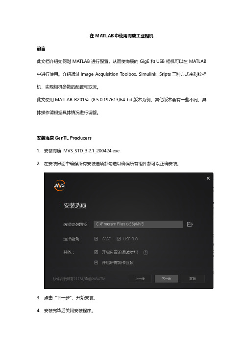
安装海康GenTL Producers1.安装海康MVS_STD_3.2.1_200424.exe2.在安装界面中确保所有安装选项都勾选以确保所有组件都可以正确安装。
3.点击“下一步”,开始安装。
4.安装完毕后关闭安装程序。
配置MATLAB GenTL 环境1.打开MATLAB,点击上方的APPS。
查看是否已安装了Image Acquisition app.2.如果Image Acquisition没有安装,需要回到Home页面打开Add-Ons->GetHardware Support Packages.3.选择Install from Internet.4.在列表中找到Image Acquisition进行安装。
5.确认是否已在MATLAB中安装了GenTL环境。
在MATLAB的Command Window中输入imaqhwinfo。
如果installedAdaptors中没有gentl,则需要安装gentl。
6.打开Home->Add-Ons->Get Hardware Support Packages.选择GenIcamInterface并安装。
在Image Acquisition中使用海康相机1.打开APPS->Image Acquisition。
所有可使用的GigE与USB相机都将会被显示在Hardware Browser中。
2.当展开相机后,相机中所支持的像素格式将会显示出来。