波浪的模拟方法
openfoam模拟波浪开了湍流模型计算总发散
openfoam模拟波浪开了湍流模型计算总发散OpenFOAM是一种自由开源的计算流体动力学(CFD)软件,被广泛用于模拟各种流体现象,包括波浪。
在波浪模拟中,湍流模型的选择对计算结果具有重要影响,其中开了湍流模型是一种被广泛使用的模型之一。
本文将从简单到复杂,由浅入深地介绍openfoam模拟波浪开了湍流模型计算总发散的相关内容。
1. 开了湍流模型简介在OpenFOAM中,湍流模型是用来模拟湍流流动的数学模型。
开了模型是一种常用的湍流模型,适用于各种湍流流动的模拟。
该模型通过求解雷诺平均的Navier-Stokes方程,考虑了湍流的能量输运和湍流粘度,并能够较准确地预测湍流流动的特性。
2. 模拟波浪中的开了模型在模拟波浪时,开了模型可以很好地捕捉湍流在波浪中的运动和变化。
通过在OpenFOAM中选择开了模型,可以对波浪的湍流特性进行准确的计算,包括湍流能量的传递、涡粘性和湍流尺度等。
这对于理解波浪的湍流行为和预测波浪的动态响应具有重要意义。
3. 开了模型计算总发散的影响在使用开了模型进行波浪模拟时,需要特别关注计算总发散的问题。
计算总发散是指在进行数值模拟计算时,由于数值不稳定性导致的计算结果发散的情况。
在使用开了模型时,由于湍流的不稳定性和复杂性,计算总发散的问题可能会显现出来。
需要对计算总发散进行深入分析和处理,以确保模拟结果的准确性和可靠性。
4. 解决计算总发散的方法为了解决计算总发散的问题,可以采取一些方法来提高模拟的稳定性和准确性。
可以对网格进行优化,提高网格的质量和分辨率,以减小数值误差;可以选择合适的时间步长和收敛准则,以确保计算过程的稳定性;另外,可以考虑使用其他湍流模型或调整开了模型的参数,以改善模拟结果的稳定性;可以通过对流场的后处理和分析,发现并纠正潜在的计算总发散问题。
总结:通过本文的介绍,我们了解了在OpenFOAM中模拟波浪开了湍流模型计算总发散的相关内容。
选择适当的湍流模型对于模拟波浪的湍流流动至关重要,而计算总发散的问题则需要引起我们的重视。
波浪理论的计算方法

波浪理论的计算方法波浪理论是用来描述海洋和湖泊中波浪的性质和行为的科学理论。
它是基于一系列基本方程和边界条件的数学模型,可以用来计算和预测波浪的高度、速度、周期等特性。
下面将介绍波浪理论的计算方法。
波浪的基本方程为水流动的欧拉方程和连续性方程,通过线性化和加入适当的边界条件,可以得到简化的一维波浪方程。
这个方程被称为波浪方程或爱舍尔-盖伊尔(Airy-Gay-Lussac)方程,是解决波浪传播和干涉问题最常用的工具。
波浪方程的一般形式如下:∂^2η/∂t^2=g∇^2η其中,∂^2η/∂t^2是波浪面随时间的加速度,g是重力加速度,∇^2是波浪面的拉普拉斯算子。
在一维情况下,波浪方程可以被进一步简化为:∂^2η/∂t^2=g∂^2η/∂x^2其中,x是水平方向的坐标。
求解这个波浪方程,可以得到波浪的解析表达式或数值解。
下面介绍几种常用的计算方法。
1. 艾尔金(Airy)线性理论:该方法假设波浪是以线性和无散动态传播的,适用于小振幅的波浪。
它利用波浪的线性性质,通过傅里叶级数展开和代数运算,可以得到波浪的频谱分布和波浪高度的概率分布。
2.快速海洋波浪传播(SWAN)模型:该模型是一种基于频谱方法的波浪模拟模型。
它将波浪场视作由多个波浪成分组成的矢量叠加,利用频谱分布和相干关系,通过解耦和复合波浪成分,可以计算出各个频段的波浪高度和方向。
3.深水波浪传播模型:该模型假设波浪在无限深水域传播,适用于大范围的波浪传播问题。
它利用波浪动能守恒和动量守恒原理,通过波浪的能量传递和波浪平衡状态的概念,可以计算出波浪随距离变化的特性。
4.海洋预报模型:该模型结合海洋动力学和波浪动力学,通过数值离散和积分方法求解波浪方程。
它将海洋和大气的相互作用考虑在内,可以计算出波浪与海流、风速等环境因素的相互作用,从而得到更准确的波浪预报结果。
这些方法都有各自的优缺点,选择适合的方法需要考虑波浪的性质、计算的精度要求和计算的效率等因素。
中科三代造浪说明书

中科三代造浪说明书一、引言中科三代造浪是一种先进的水波发生装置,能够模拟各种自然条件下的海浪,广泛应用于海洋工程、海洋科学研究、船舶设计等领域。
本说明书将详细介绍中科三代造浪的原理、结构、使用方法以及注意事项。
二、原理中科三代造浪是通过机械振荡产生波浪的装置。
其主要原理是利用悬挂在装置内部的振荡体产生机械振动,进而将振动传递给水体,形成波浪。
振荡体的振动频率、振幅和振动方式可以根据需要进行调节,从而实现不同条件下的波浪模拟。
三、结构中科三代造浪由振荡体、传动系统、控制系统和水槽组成。
振荡体是装置的核心部分,它通过传动系统与控制系统相连,将机械能转化为振动能。
传动系统通过传动轴将振动能传递给水槽中的水体,使其产生波浪。
控制系统可以调节振荡体的振动频率和振幅,从而实现不同波浪条件下的模拟。
四、使用方法1. 准备工作:检查中科三代造浪装置是否完好,确保各部分连接牢固。
2. 装置调试:根据实验需求,调整振荡体的振动频率和振幅,以及振动方式。
3. 水槽填充:将水槽填满水,确保水位稳定。
4. 启动装置:打开控制系统的电源,启动中科三代造浪装置。
5. 观测记录:观察水槽中的波浪情况,并记录相关数据。
6. 实验结束:关闭中科三代造浪装置,清理水槽及相关设备。
五、注意事项1. 在使用中科三代造浪装置前,务必熟悉操作手册,并由专业人员指导操作。
2. 使用时要注意安全,避免发生人身伤害或设备损坏。
3. 注意装置的维护保养,定期检查各部件的工作状态,及时更换损坏的零部件。
4. 使用中科三代造浪装置时,应根据实验需求调整振荡体的参数,以达到所需的波浪模拟效果。
5. 使用结束后,及时清理水槽,防止水质污染和设备损坏。
六、总结通过本说明书的介绍,我们了解了中科三代造浪的原理、结构、使用方法以及注意事项。
中科三代造浪作为一种先进的水波发生装置,具有广泛的应用前景和重要的实际意义。
相信在今后的研究和应用中,中科三代造浪将发挥更大的作用,为海洋工程、海洋科学研究等领域带来更多的突破和进展。
一种改进的基于FLUENT的三维波浪水槽模拟方法

在海洋和海岸港 口工程中 ,船舶 和海洋结构物 的 部分试验研究需要在波浪水槽 中进行 。随着数值计算 方法和硬件的发展进步 ,采用计算机模拟波浪水槽 的 方法研究波浪传播及其对船舶 和海洋结构物 的影响 已 变得越来越普遍。 国、内外学者针对数值波浪水槽 的 相关研究主要集 中在波浪的运动特征 和形态 、波浪对 结构物 的作用和造波模式等方面 ,并取得 了一定 的成 果 。在波浪数值模拟方面 ,通 常采用 的方程包括 :基 于势流理论 的 L a p l a c e 方 程 、综合 考虑折 射和绕 流 的 缓坡方 程 、B o u s s i n e s q方程 和 N — s方 程等 。 。由于 某些方程对流体黏性或忽略不计 ,或以能量耗散项 的 形式计人 ,在海浪模拟方面存 在一定 的失真 。而采用 黏性流体运动 的 N . s方程进行建模和分析 ,可以完全 考虑流体 的运动规律 ,更好地模拟海 浪的运 动 。
Ab s t r a c t :B y a n a l y z i n g t h e e x i s t i n g w a v e t a n k s i mu l a t i o n me t h o d, a n e n e r g y f u n c t i o n u s e d i n t h e w a v e a b s o r p t i o n a r e a w a s o f - f e r e d wh e n u s i n g F L U NE T t o s i mu l a t e t h e 3 - D t a n k .T h e e n e r g y f u n c t i o n wa s p u t i n t o t h e F L UE NT s o l v e r ,a n d t h e r e s u l t s w e r e t o m— p a r e d wi t h e x p e r i me n t a l r e s u l t s .T h e o p t i ma l wa v e a t t e n u a t i o n c o e ic f i e n t o f e n e r y g f u n c t i o n w a s d e c i d e d t h r o u g h t h e c o mp a r e .T h i s me t h o d c a n b e u s e d t o o p t i mi z e t h e 3 - D t a n k p e r f e c t l y ,a n d t h e s i mu l a t i o n r e s u l t i s s i mi l a r w i t h e x p e r i e n c e r e s u l t .
海面波浪模拟MATLAB
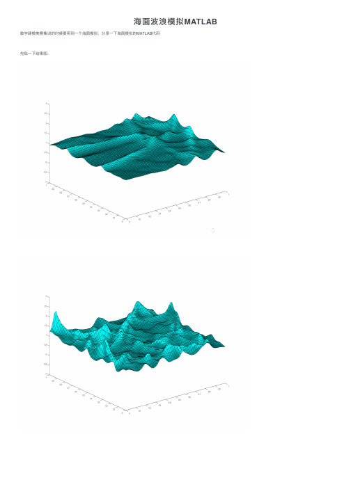
海⾯波浪模拟MATLAB 数学建模美赛集训的时候要⽤到⼀个海⾯模拟,分享⼀下海⾯模拟的MATLAB代码先贴⼀下结果图:下⾯是源代码~~~1function waterwave234n = 64; % grid size5g = 9.8; % gravitational constant6dt = 0.01; % hardwired timestep7dx = 1.0;8dy = 1.0;9nplotstep = 8; % plot interval10ndrops = 5; % maximum number of drops11dropstep = 500; % drop interval12D = droplet(1.5,21); % simulate a water drop1314% Initialize graphics1516[surfplot,top,start,stop] = initgraphics(n);1718% Outer loop, restarts.1920while get(stop,'value') == 021 set(start,'value',0)2223 H = ones(n+2,n+2); U = zeros(n+2,n+2); V = zeros(n+2,n+2);24 Hx = zeros(n+1,n+1); Ux = zeros(n+1,n+1); Vx = zeros(n+1,n+1);25 Hy = zeros(n+1,n+1); Uy = zeros(n+1,n+1); Vy = zeros(n+1,n+1);26 ndrop = ceil(rand*ndrops);27 nstep = 0;2829 % Inner loop, time steps.3031 while get(start,'value')==0 && get(stop,'value')==032 nstep = nstep + 1;3334 % Random water drops35 if mod(nstep,dropstep) == 0 && nstep <= ndrop*dropstep36 w = size(D,1);37i = ceil(rand*(n-w))+(1:w);38j = ceil(rand*(n-w))+(1:w);39H(i,j) = H(i,j) + rand*D;40 end4142 % Reflective boundary conditions43 H(:,1) = H(:,2); U(:,1) = U(:,2); V(:,1) = -V(:,2);44H(:,n+2) = H(:,n+1); U(:,n+2) = U(:,n+1); V(:,n+2) = -V(:,n+1); 45H(1,:) = H(2,:); U(1,:) = -U(2,:); V(1,:) = V(2,:);46H(n+2,:) = H(n+1,:); U(n+2,:) = -U(n+1,:); V(n+2,:) = V(n+1,:);4748% First half step4950 % x direction51 i = 1:n+1;52j = 1:n;5354% height55 Hx(i,j) = (H(i+1,j+1)+H(i,j+1))/2 - dt/(2*dx)*(U(i+1,j+1)-U(i,j+1));5657 % x momentum58 Ux(i,j) = (U(i+1,j+1)+U(i,j+1))/2 - ...59 dt/(2*dx)*((U(i+1,j+1).^2./H(i+1,j+1) + g/2*H(i+1,j+1).^2) - ...60 (U(i,j+1).^2./H(i,j+1) + g/2*H(i,j+1).^2));6162 % y momentum63 Vx(i,j) = (V(i+1,j+1)+V(i,j+1))/2 - ...64 dt/(2*dx)*((U(i+1,j+1).*V(i+1,j+1)./H(i+1,j+1)) - ...65 (U(i,j+1).*V(i,j+1)./H(i,j+1)));6667 % y direction68 i = 1:n;69j = 1:n+1;7071% height72 Hy(i,j) = (H(i+1,j+1)+H(i+1,j))/2 - dt/(2*dy)*(V(i+1,j+1)-V(i+1,j));7374 % x momentum75 Uy(i,j) = (U(i+1,j+1)+U(i+1,j))/2 - ...76 dt/(2*dy)*((V(i+1,j+1).*U(i+1,j+1)./H(i+1,j+1)) - ...77 (V(i+1,j).*U(i+1,j)./H(i+1,j)));78 % y momentum79 Vy(i,j) = (V(i+1,j+1)+V(i+1,j))/2 - ...80 dt/(2*dy)*((V(i+1,j+1).^2./H(i+1,j+1) + g/2*H(i+1,j+1).^2) - ...81 (V(i+1,j).^2./H(i+1,j) + g/2*H(i+1,j).^2));8283 % Second half step84 i = 2:n+1;85j = 2:n+1;8687% height88 H(i,j) = H(i,j) - (dt/dx)*(Ux(i,j-1)-Ux(i-1,j-1)) - ...89 (dt/dy)*(Vy(i-1,j)-Vy(i-1,j-1));90 % x momentum91 U(i,j) = U(i,j) - (dt/dx)*((Ux(i,j-1).^2./Hx(i,j-1) + g/2*Hx(i,j-1).^2) - ...92 (Ux(i-1,j-1).^2./Hx(i-1,j-1) + g/2*Hx(i-1,j-1).^2)) ...93 - (dt/dy)*((Vy(i-1,j).*Uy(i-1,j)./Hy(i-1,j)) - ...94 (Vy(i-1,j-1).*Uy(i-1,j-1)./Hy(i-1,j-1)));95 % y momentum96 V(i,j) = V(i,j) - (dt/dx)*((Ux(i,j-1).*Vx(i,j-1)./Hx(i,j-1)) - ...97 (Ux(i-1,j-1).*Vx(i-1,j-1)./Hx(i-1,j-1))) ...98 - (dt/dy)*((Vy(i-1,j).^2./Hy(i-1,j) + g/2*Hy(i-1,j).^2) - ...99 (Vy(i-1,j-1).^2./Hy(i-1,j-1) + g/2*Hy(i-1,j-1).^2));100101 % Update plot102 if mod(nstep,nplotstep) == 0103 C = abs(U(i,j)) + abs(V(i,j)); % Color shows momemtum104 t = nstep*dt;105tv = norm(C,'fro');106set(surfplot,'zdata',H(i,j),'cdata',C);107 set(top,'string',sprintf('t = %6.2f, tv = %6.2f',t,tv))108drawnow109 end110111 if all(all(isnan(H))), break, end % Unstable, restart112 end113end114close(gcf)115116% ------------------------------------117118function D = droplet(height,width)119% DROPLET 2D Gaussian120% D = droplet(height,width)121[x,y] = ndgrid(-1:(2/(width-1)):1);122 D = height*exp(-5*(x.^2+y.^2));123124% ------------------------------------125126function [surfplot,top,start,stop] = initgraphics(n);127% INITGRAPHICS Initialize graphics for waterwave.128% [surfplot,top,start,stop] = initgraphics(n)129% returns handles to a surface plot, its title, and two uicontrol toggles. 130131 clf132 shg133 set(gcf,'numbertitle','off','name','Shallow_water')134 x = (0:n-1)/(n-1);135surfplot = surf(x,x,ones(n,n),zeros(n,n));136grid off137 axis([0 1 0 1 -1 3])138 caxis([-1 1])139 shading faceted140 c = (1:64)'/64;141cyan = [0*c c c];142 colormap(cyan)143 top = title('Click start');144 start = uicontrol('position',[20 20 80 20],'style','toggle','string','start'); 145 stop = uicontrol('position',[120 20 80 20],'style','toggle','string','stop');。
Fluent二维波浪模拟教程
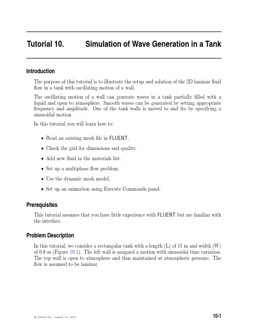
Tutorial10.Simulation of Wave Generation in a TankIntroductionThe purpose of this tutorial is to illustrate the setup and solution of the2D laminarfluid flow in a tank with oscillating motion of a wall.The oscillating motion of a wall can generate waves in a tank partiallyfilled with a liquid and open to atmosphere.Smooth waves can be generated by setting appropriate frequency and amplitude.One of the tank walls is moved to and fro by specifying a sinusoidal motion.In this tutorial you will learn how to:•Read an existing meshfile in FLUENT.•Check the grid for dimensions and quality.•Add newfluid in the materials list.•Set up a multiphaseflow problem.•Use the dynamic mesh model.•Set up an animation using Execute Commands panel.PrerequisitesThis tutorial assumes that you have little experience with FLUENT but are familiar with the interface.Problem DescriptionIn this tutorial,we consider a rectangular tank with a length(L)of15m and width(W) of0.8m(Figure10.1).The left wall is assigned a motion with sinusoidal time variation.The top wall is open to atmosphere and thus maintained at atmospheric pressure.The flow is assumed to be laminar.Simulation of Wave Generation in a TankFigure10.1:Problem SchematicPreparation1.Copy the meshfile,wave.msh and libudf folder to your working directory.2.Start the2D double precision solver of FLUENT.Setup and SolutionStep1:Grid1.Read the gridfile,wave.msh.File−→Read−→Case...FLUENT will read the meshfile and report the progress in the console window.2.Check the grid.Grid−→CheckThis procedure checks the integrity of the mesh.Make sure the reported minimumvolume is a positive number.3.Check the scale of the grid.Grid−→Scale...Simulation of Wave Generation in a Tank Check the domain extents to see if they correspond to the actual physical dimensions.If not,the grid has to be scaled with proper units.4.Display the grid(Figure10.2).Display−→Grid...(a)Click Colors....The Grid Colors panel opens.i.Under Options,enable Color by ID.ii.Click Close.(b)In the Grid Display panel,click Display(c)Zoom in near the moving-wall(Figure10.3).Simulation of Wave Generation in a TankFigure10.2:Grid DisplayFigure10.3:Grid Display(Close-up of moving-wall)Simulation of Wave Generation in a TankStep2:Models1.Specify the solver settings.Define−→Models−→Solver...(a)Under Time,enable Unsteady(b)Under Transient Controls,enable Non-Iterative Time Advancement.(c)Click OK.2.Enable VOF multiphase model.Define−→Models−→Multiphase...Simulation of Wave Generation in a Tank(a)Under Model,enable Volume of Fluid.The panel expands to show the other settings related to VOF model.Retainthe other settings as default.(b)Click OK.Step3:MaterialsDefine−→Materials...1.Add liquid water to the list offluid materials by copying it from the materialsdatabase.Simulation of Wave Generation in a Tank(a)Click Fluent Database....Fluent Database Materials panel opens.Simulation of Wave Generation in a Tanki.Select water-liquid(h2o<l>)from the Fluent Fluid Materials list.Scroll down to view water-liquid.ii.Click Copy and close the panel.(b)Click Change/Create and close the panel.Step4:PhasesDefine−→Phases...1.Set air as primary phase and water as secondary phase.(a)Under Phase,select phase-1.The Type will be shown as primary-phase.(b)Click Set....i.Change Name to air.ii.Select air in the Phase Material drop-down list.iii.Click OK.(c)Similarly,change the Name of phase-2to water and set its Type to water-liquid.(d)Close the Phases panel.Simulation of Wave Generation in a TankStep5:Operating ConditionsDefine−→Operating Conditions...1.Set the gravitational acceleration.(a)Enable Gravity.(b)Under Gravitational Acceleration,set Y to-9.81m/s2.As the tank bottom is perpendicular to Y axis,gravity points in the negativeY direction.2.Set the operating density.(a)Under Variable-Density Parameters,enable Specified Operating Density.(b)Retain the default density of1.225kg/m3.Set the operating density to the density of the lighter phase.This excludesthe build-up of hydrostatic pressure within the lighter phase,improving theround-offaccuracy for the momentum balance.3.Set the reference pressure location.(a)Under Reference Pressure Location,retain the default value of zero for both Xand Y.This location corresponds to a region where thefluid will always be100%ofone of the phases(water).If it is not,it is recommended to change the regionto a appropriate location where the pressure value does not change much overtime.This condition is essential for smooth and rapid convergence.4.Click OK to accept the settings and close the panel.Simulation of Wave Generation in a TankStep6:Boundary ConditionsFLUENT maintains zero velocity condition on all the walls.Also,the pressure condition for outlet boundary at the top is set by default to zero gauge(or atmospheric).Hence, there is no need to change the boundary conditions.Retain all the boundary conditions as default.Step7:UDF LibraryDefine−→User-Defined−→Functions−→Compiled...1.Click Load to load the UDF library.The sinusoidal wall motion will be assigned using user defined function.A compiledUDF library named libudf is created for this purpose.Step8:Dynamic Mesh Model1.Set the dynamic mesh parameters.Define−→Dynamic Mesh−→Parameters...(a)Under Models,enable Dynamic Mesh.The panel expands.(b)Under Mesh Methods,disable Smoothing and enable Layering.(c)Under the Layering tab,set Collapse Factor to0.4.(d)Click OK.2.Set the dynamic mesh zones.Define−→Dynamic Mesh−→Zones...(a)Under Zone Names,select moving-wall.(b)Under Type,retain the default selection of Rigid Body.(c)Under Meshing Options tab,set Cell Height to0.008m.This is the average size of the cell normal to the moving wall.(d)Click Create and close the panel.Step9:Solution1.Retain the default solution controls.Solve−→Controls−→Solution...Solve−→Initialize−→Initialize...(a)Click Init and close the panel.The complete domain is now initialized with air.The water level required at start(t=0)can be patched.3.Create a register marking the region of initial water level.Adapt−→Region...(a)Set X Max to be15m.(b)Set Y Max to be0.5m.(c)Click Mark and close the panel.FLUENT displays the following message in the console:8510cells marked for refinement,0cells marked for coarsening.4.Patch the initial water level.Solve−→Initialize−→Patch...(a)Under Registers to Patch,select hexahedron-r0.(b)Under Phase,select water.(c)Under Variable,select Volume Fraction.(d)Set Value to1.(e)Click Patch and close the panel.5.Display the zone motion to check the movement of moving-wall.(a)Display the grid(Figure10.4).Display−→Grid...i.Under Surfaces,deselect default-interior.Zoom-in the graphics window to get the view as shown in Figure10.4.ii.Click Display.Figure10.4:Grid Display Outline at t=0(b)Display the zone motion.Display−→Zone Motion...i.Under Motion History Integration,set Time Step to0.001.ii.Set Number of Steps to300.iii.Click Integrate.iv.Under Preview Controls,set Time Step to0.001.v.Set Number of Steps to300.vi.Click Preview to observe the wall motion.vii.Close the Zone Motion panel.6.View the contours of volume fraction for water(Figure10.5).Display−→Contours...(a)Select Phases...and Volume Fraction in the Contours of drop-down lists.(b)Under Phase,select water.(c)Under Options,enable Filled.(d)Click Display and close the panel.Figure10.5:Contours of Volume Fraction for Water7.Enable the plotting of residuals during the calculation.Solve−→Monitors−→Residuals...(a)Under Options,enable Plot.(b)Under Plotting,set Iterations to10.This will display residuals for only the last10iterations.(c)Click OK.8.Set hardcopy settings.File−→Hardcopy...(a)Under Format,select TIFF.(b)Under Coloring,select Color.(c)Click Apply.(d)Click Preview.The background of graphics window is changed to white.FLUENT will displaya question dialog box asking you whether to reset the window.(e)Click Yes in the Question dialog box.(f)Close the panel.9.Set the commands to capture the images of contours.You need to use Text User Interface(TUI)commands to achieve this.For most of the graphical commands,corresponding TUI commands are available.Solve−→Execute Commands...(a)Set the number of Defined Commands to3.(b)Enable On option for all the commands.(c)Under Every,set7for all the commands.(d)Under When,set Time Step for all the commands.(e)For command-1,specify the Command as:display set-window1This command will make the window-1active.(f)For command-2,specify the Command as:display contour water vof01This command will display the contours of water volume fraction in the activewindow.(g)For command-1,specify the Command as:display hard-copy"vof-%t.tif"This command will save the image in the TIF format.The%t option gets replaced with the time step number,when the imagefileis saved.The TIFfiles saved can then be used to create a movie.For theinformation on converting TIFfile to an animationfile,refer to/cfm/graphics01.htm(h)Click OK to accept the settings and close the panel.10.Set the surface monitors.Solve−→Monitors−→Surface...(a)Increase the number of Surface Monitors to1.(b)Enable Plot for monitor-1.(c)Under Every,select Time Step.(d)Click on Define...next to monitor-1.(e)Select Area Weighted Average in the Report Type drop-down list.(f)Select Grid and X-Coordinate in the Report of drop-down list.(g)Under Surfaces,select moving-wall.(h)Click OK to close both the panels.11.Save the case and datafiles(wave-init.cas.gz and wave-init.dat.gz).File−→Write−→Case&Data...Retain the default Write Binary Files option so that you can write a binaryfile.The .gz extension will save zippedfiles on both,Windows and UNIX platforms.12.Start the calculation.Solve−→Iterate...(a)Set the Time Step Size as0.001s(b)Set Number of Time Steps to4000.(c)Click Iterate.Figure10.6:Scaled Residuals13.Save the case and datafiles(wave-4000.cas.gz and wave-4000.dat.gz).Figure10.7:Monitor Plot of Area Weighted Average on moving-wallStep10:Postprocessing1.Displayfilled contours of static pressure(Figure10.8).Display−→Contours...(a)Select Pressure...and Static Pressure in the Contours of drop-down lists.(b)Click Display.The pressure at the bottom of the tank is maximum and goes on decreasingtowards the top.This shows the variation of hydrostatic pressure due to theheight of the liquid.Figure10.8:Contours of Static PressureSummaryThe dynamic mesh model is used to apply periodic sinusoidal motion to the wall.This generates a wave in thefluid.The VOF model is used to track the air-water interface and consequently the wave motion.Non-iterative time advancement(NITA)was used to reduce the run time of transient simulation.Images displaying contours of water phase were captured to visualize the transient effects.References1.Flow Around the Itsukushima Gate,an example from Fluent Inc.Marketing Cata-log,2003.Exercises/Discussions1.Run the simulation for longerflow time to check the wave pattern.2.Try running the simulation without non-iterative time advancement(NITA)option.(a)Are theflow patterns different?(b)Compare the wall clock time taken to reach the sameflow time.3.Run the simulation using variable time step option.4.Try different motions to the wall and observe wave patterns.This will need specific C compiler to create UDF library from the source code.5.What other situation can be simulated using the same meshfile?Links for Further Reading•http://www.prads2004.de/pdf/027.pdf•http://www.prads2004.de/pdf/138.pdf•http://www.math.rug.nl/∼veldman/preprints/OMAE2004-51084.pdf。
c4d波浪效果的公式
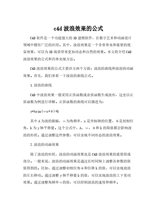
c4d波浪效果的公式C4D软件是一个功能强大的3D建模软件,在数字艺术和动画设计领域中拥有广泛的应用。
其中,波浪效果是一个非常常见和重要的视觉效果,可以为3D场景带来更加动态和自然的效果。
本文将介绍C4D 波浪效果的公式和具体实现方法。
C4D波浪效果的公式主要涉及两个方面:波浪的曲线和波浪的动画效果。
首先,我们来看一下波浪的曲线公式。
1.波浪的曲线C4D中波浪效果一般采用正弦函数或余弦函数生成波形,这里以正弦函数为例进行讲解。
正弦函数的曲线可以描述为:y=Asin(ωx+φ)+k其中A为波的振幅,ω为角频率,x是坐标轴的位置,φ是初相位角,k为y轴平移量。
这个公式中,A、ω、φ和k的取值都会影响波浪的形状。
通过调整这些参数,可以实现不同形态的波浪效果。
2.波浪的动画效果除了波浪的形状,波浪的动画效果也是C4D波浪效果的重要组成部分。
一般来说,波浪的动画效果是通过在时间轴上调整各参数的取值得到的。
比如,通过调整初相位角φ和位移k的值,可以实现波浪的左右移动。
通过调整y轴平移量k的值,可以实现波浪的上下晃动效果。
通过调整角频率ω的值,可以控制波浪的速度和频率。
除了以上两个方面的公式,还有一个重要的部分是具体的实现方法。
下面将详细介绍C4D波浪效果的实现方法。
1.新建一个平面对象,设置其细分格数2.插入一个位图材质,选择合适的波浪图片3.在材质贴图中设置偏移量和缩放比例4.将该材质应用到平面对象上5.在材质编辑器中选择“纹理工具”,调整位移和缩放的数值6.进行动画效果的制作:选择平面对象,点击“模拟帧”按钮,在时间轴中选择开始帧和结束帧,调整参数,生成动画效果以上是C4D波浪效果的具体实现方法。
通过以上步骤,可以轻松制作出各种不同形态和动画效果的波浪。
需要注意的是,在实际制作过程中,还需要不断调整参数,尝试不同的取值组合,才能达到最佳的效果。
综上所述,C4D波浪效果是一个非常常见和重要的视觉效果,其公式涉及波浪的曲线和动画效果,还需要具体的实现方法。
波浪模型试验规程

波浪模型试验规程什么是波浪模型试验?波浪模型试验是海洋航行中预测船舶航行阻力的一种测试方法,它由模型船只所拟仿的洋流以及模拟波浪组成。
这种方法可以准确地反映船舶在不同环境条件下的行为,从而给船舶设计和海上安全提供支持。
波浪模型试验的目的是通过对模型船行为的测量来获得关于船舶设计性能的准确数据。
它能够仔细研究船舶的耐久性,安全性,稳定性和机动性,从而提高船舶设计和海上安全性。
此外,波浪模型测试还可以应用于评估船舶阻力和受力、能量损失以及船体噪声、振动的测量。
通过对模型船的多参量检验,可以深入了解船舶的状态变化,提高船舶的设计和操作水平。
因此,波浪模型试验是设计和使用船舶的必要环节,被认为是海洋航行的核心技术。
本文就如何进行波浪模型试验并得出有用结论给出介绍。
一、实施波浪模型试验的准备工作1)波浪模型试验的模型选择:需要根据模型船的实际海洋环境条件选择合适的模型。
通常,应该考虑模型船的总体形状、体积、尺寸和重量等因素。
2)模型内部布置:模型实验室一般提供合适的研究空间,基本上应该包括船舶设备,通风及空调系统,电气设备,水文和水力设备,以及研究所需的有关设备。
在模型实验室中,应该考虑设备的安全性,舒适性和可操作性,以便尽可能地减少实验的误差。
3)水池准备:水池也是实验的重要组成部分。
它应该具有足够的洗涤能力,可以满足不同任务要求,并可以模拟真实海洋环境。
在使用大水池时,应确保池壁和底板清洁,设备稳定,以确保实验结果的可靠性。
4)模型准备:模型的准备应考虑模型的总体结构、重量分布和装配细节等因素,确保准确无误。
此外,还应考虑模型的表面处理,力学实验仪器和仪器仪表设备设置,以确保测量准确。
二、波浪模型试验步骤及其应用1)模型安装:模型安装是实验中最重要的一步,应确保模型正确地安装在水池中,并且与水池壁吻合,不能有任何松动,否则实验结果会受到影响。
2)流量精度调整:波浪模型的流量精度是实验的重要参数,它影响着实验的准确性,也是模型实验的关键环节,应该确保它的精度和可靠性。
- 1、下载文档前请自行甄别文档内容的完整性,平台不提供额外的编辑、内容补充、找答案等附加服务。
- 2、"仅部分预览"的文档,不可在线预览部分如存在完整性等问题,可反馈申请退款(可完整预览的文档不适用该条件!)。
- 3、如文档侵犯您的权益,请联系客服反馈,我们会尽快为您处理(人工客服工作时间:9:00-18:30)。
T ()
3. 产生不规则波 造波板控制信号的计算:
N
不规则波波面: (t) an cos(n t n ) n 1
造波板的运动:
stroke(t )
N 1
an
T (n )
sin(n t
n )
an 2s()
an 各个组成波的振幅 s() 波浪的频谱 n 波浪的随机初始相位
T1 ( )
e
R()
e 造波板运动 R(): 控制造波板信号幅值(电压)
可通过标定的方式确定 ,近似为线性关系。
(2)造波机水动力传递函数:
T2
()
a0 e
a0 造波板前波浪的振幅 e: 造波板运动幅值
通过波浪理论推导确定,对于推板式造波机:
T2 ()
4sinh2 (kh) 2kh sinh(2kh)
实验室产生海浪的理论方法
1. 确定造波机的传递函数:
造波机的传递函数:表示所产生的波浪 a与造波板运动e之间的关系:
T () a
e
T1() T2 () T3 ()
T1(): 造波机系统的机械传递函数 T2(): 水动力传递函数 T3(): 波浪传播变形函数
(1) 造波机系统的机械传递函数::
k 波浪的波数;h 水深。
(3)波浪传播变形函数:
T3 ()
a a0
a 模型断面波浪振幅
a0 造波板前波浪的振幅
可通过波浪传播理论计算确定。
造波机产生波浪的控制过程中只考 虑水动力传递函数:
T () T2 ()
2. 产生规则波 造波板控制信号的计算:
规则波波面: (t) a cos(t 0 ) 造波板的运动: stroke(t) E sin(t 0 )