2002The influence of different irradiation sources on the treatment of nitrobenzene - 副本

合集下载

医学研究生学报

第17卷　第4期医学研究生学报 Vol.17　No.4　2004年4月 Journal of Medical Postgraduates Apr.2004・综述・放射性核素近距离治疗肿瘤的研究新进展高立宁综述,　杜明华审校(东南大学附属中大医院核医学科,江苏南京210009)摘要:　放射性粒子组织间近距离治疗肿瘤虽已取得成功,但仍有许多问题尚未解决。

该文回顾性综述了近距离治疗肿瘤的最新研究成果,包括放射性核素的选择、不同源的形式对剂量学分布的影响、治疗质量的保证、近距离治疗在空腔脏器肿瘤治疗中的应用以及近距离治疗的新趋势和展望。

关键词:　放射性核素;　近距离治疗;　肿瘤中图分类号:　R730.55 文献标识码:　A 文章编号:　100828199(2004)0420373203ΞNew progress in the research of radionuclides for tumor brachytherapyG AO Li2ning review i ng,DU Ming2hua checki ng(Depart ment of N uclear Medici ne,ZhongDa Hospital A f f iliated Southeast U niversity,N anji ng 210009,Jiangsu,Chi na)Abstract:　Interstitial brachytherapy with radionuclide seeds has been successfully used for the treat2 ment of cancer.But there are some problems remain to be solved.This review focus on some recent advances in the study of brachytherapy,including the option of radionuclides,the influence of dosage distribution by using different sources,the quality assurance,the application of brachytherapy in hol2 low visceral neoplasm,and new trends in brachytherapy.K ey w ords:　Radionuclide;　Brachytherapy;　Tumor0　引言近年来,随着科学技术的进步和医学生命科学的发展,新的放射性核素(如125I、198Au、103Pd、241Am、252C f)研究成功并用于治疗;同时新的技术也如雨后春笋般涌现出来,使得放射性核素组织间种植近距离治疗肿瘤的技术日臻完善。

放疗技术的发展历史

放疗技术的发展历史
放疗技术的发展历史可以追溯到19 世纪末期。

以下是放疗技术发展的历程：
1、1895 年：德国物理学家威廉·康拉德·伦琴发现了X 射线，这为放疗技术的发展奠定了基础。

2、1902 年：居里夫妇发现了镭元素，并发明了用于治疗肿瘤的镭放射疗法。

3、20 世纪30 年代：直线加速器的出现使得放疗能够治疗深部肿瘤。

4、20 世纪50 年代：钴-60 放射性同位素的应用使得放疗更加安全和方便。

5、20 世纪70 年代：计算机技术的发展使得放疗可以更精确地瞄准肿瘤，减少对正常组织的伤害。

6、20 世纪80 年代：三维适形放疗技术的出现，进一步提高了放疗的精度和效果。

7、21 世纪初：调强放疗和质子放疗等先进技术的应用，使放疗更加个体化和精准。

随着科技的不断进步，放疗技术仍在不断发展和完善，为癌症治疗提供了重要的手段。

ASTM_A262-2002a(硝酸全浸65%)

Designation:A262–02a An American National Standard Standard Practices forDetecting Susceptibility to Intergranular Attack in Austenitic Stainless Steels1This standard is issued under theﬁxed designation A262;the number immediately following the designation indicates the year oforiginal adoption or,in the case of revision,the year of last revision.A number in parentheses indicates the year of last reapproval.Asuperscript epsilon(e)indicates an editorial change since the last revision or reapproval.This standard has been approved for use by agencies of the Department of Defense.1.Scope*1.1These practices cover the followingﬁve tests:1.1.1Practice A—Oxalic Acid Etch Test for Classiﬁcation of Etch Structures of Austenitic Stainless Steels(Sections3to 7,inclusive),1.1.2Practice B—Ferric Sulfate–Sulfuric Acid Test for Detecting Susceptibility to Intergranular Attack in Austenitic Stainless Steels(Sections8to14,inclusive),1.1.3Practice C—Nitric Acid Test for Detecting Suscepti-bility to Intergranular Attack in Austenitic Stainless Steels (Sections15to21,inclusive),1.1.4Practice E—Copper–Copper Sulfate–Sulfuric Acid Test for Detecting Susceptibility to Intergranular Attack in Austenitic Stainless Steels(Sections22to31,inclusive),and 1.1.5Practice F—Copper–Copper Sulfate–50%Sulfuric Acid Test for Detecting Susceptibility to Intergranular Attack in Molybdenum-Bearing Cast Austenitic Stainless Steels(Sec-tions32to38,inclusive).1.2The following factors govern the application of these practices:1.2.1Susceptibility to intergranular attack associated with the precipitation of chromium carbides is readily detected in all six tests.1.2.2Sigma phase in wrought chromium-nickel-molybdenum steels,which may or may not be visible in the microstructure,can result in high corrosion rates only in nitric acid.1.2.3Sigma phase in titanium or columbium stabilized alloys and cast molybdenum-bearing stainless alloys,which may or may not be visible in the microstructure,can result in high corrosion rates in both the nitric acid and ferric sulfate-–sulfuric acid solutions.1.3The oxalic acid etch test is a rapid method of identify-ing,by simple etching,those specimens of certain stainless steel grades that are essentially free of susceptibility to intergranular attack associated with chromium carbide precipi-tates.These specimens will have low corrosion rates in certain corrosion tests and therefore can be eliminated(screened)from testing as“acceptable.”1.4The ferric sulfate–sulfuric acid test,the copper–copper sulfate–50%sulfuric acid test,and the nitric acid test are based on weight loss determinations and,thus,provide a quantitative measure of the relative performance of specimens evaluated.In contrast,the copper–copper sulfate–16%sulfuric acid test is based on visual examination of bend specimens and,therefore, classiﬁes the specimens only as acceptable or nonacceptable.1.5In most cases either the24-h copper–copper sul-fate–16%sulfuric acid test or the120-h ferric sulfate–sulfuric acid test,combined with the oxalic acid etch test,will provide the required information in the shortest time.All stainless grades listed in the accompanying table may be evaluated in these combinations of screening and corrosion tests,except those specimens of molybdenum-bearing grades(for example 316,316L,317,and317L),which represent steel intended for use in nitric acid environments.1.6The240-h nitric acid test must be applied to stabilized and molybdenum-bearing grades intended for service in nitric acid and to all stainless steel grades that might be subject to end grain corrosion in nitric acid service.1.7Only those stainless steel grades are listed in Table1for which data on the application of the oxalic acid etch test and on their performance in various quantitative evaluation tests are available.1.8Extensive test results on various types of stainless steels evaluated by these practices have been published in Ref(1).2 1.9The values stated in SI units are to be regarded as standard.The inch-pound equivalents are in parentheses and may be approximate.1.10This standard does not purport to address all of the safety problems,if any,associated with its use.It is the responsibility of the user of this standard to establish appro-priate safety and health practices and determine the applica-bility of regulatory limitations prior to use.(Speciﬁc precau-tionary statements are given in5.6,11.1.1,11.1.9,and35.1.)1These practices are under the jurisdiction of ASTM Committee A01on Steel, Stainless Steel and Related Alloys and are the direct responsibility of Subcommittee A01.14on Methods of Corrosion Testing.Current edition approved Nov.10,2002.Published December2002.Originally approved st previous edition approved in2002as A262–02.2The boldface numbers in parentheses refer to the list of references found at the end of these practices.1*A Summary of Changes section appears at the end of this standard. Copyright©ASTM International,100Barr Harbor Drive,PO Box C700,West Conshohocken,PA19428-2959,United States.2.Referenced Documents 2.1ASTM Standards:A 370Test Methods and Deﬁnitions for Mechanical Testing of Steel Products 32.2ISO Standard:ISO 5651-2Determination of Resistance to Intergranular Corrosion of Stainless Steels—Part 2:Ferritic,Austenitic,and Ferritic-Austenitic (Duplex)Stainless Steels—Corrosion Test in Media Containing Sulfuric Acid 4PRACTICE A—OXALIC ACID ETCH TEST FOR CLASSIFICATION OF ETCH STRUCTURES OFAUSTENITIC STAINLESS STEELS 23.Scope3.1The oxalic acid etch test is used for acceptance of material but not for rejection of material.This may be used in connection with other evaluation tests to provide a rapid method for identifying those specimens that are certain to be free of susceptibility to rapid intergranular attack in these other tests.Such specimens have low corrosion rates in the various hot acid tests,requiring from 4to 240h of exposure.These specimens are identiﬁed by means of their etch structures,which are classiﬁed according to the following criteria:3.2The oxalic acid etch test may be used to screen specimens intended for testing in Practice B—Ferric Sulfate-–Sulfuric Acid Test,Practice C—Nitric Acid Test,Practice E—Copper–Copper Sulfate–16%Sulfuric Acid Test,and Practice F—Copper–Copper Sulfate–50%Sulfuric Acid Test.3.2.1Each practice contains a table showing which classi-ﬁcations of etch structures on a given stainless steel grade are equivalent to acceptable,or possibly nonacceptable perfor-mance in that particular test.Specimens having acceptable etch structures need not be subjected to the hot acid test.Specimens having nonacceptable etch structures must be tested in the speciﬁed hot acid solution.3.3The grades of stainless steels and the hot acid tests for which the oxalic acid etch test is applicable are listed in Table 2.3.4Extra-low–carbon grades,and stabilized grades,such as 304L,316L,317L,321,and 347,are tested after sensitizing heat treatments at 650to 675°C (1200to 1250°F),which is the range of maximum carbide precipitation.These sensitizing treatments must be applied before the specimens are submitted to the oxalic acid etch test.The most commonly used sensitiz-ing treatment is 1h at 675°C (1250°F).4.Apparatus4.1Source of Direct Current —Battery,generator,or recti-ﬁer capable of supplying about 15V and 20A.4.2Ammeter —Range 0to 30A (Note 1).4.3Variable Resistance (Note 1).4.4Cathode —A cylindrical piece of stainless steel or,preferably,a 1-qt (0.946-L)stainless steel beaker.4.5Large Electric Clamp —To hold specimen to be etched.4.6Metallurgical Microscope —For examination of etched microstructures at 250to 500diameters.3Annual Book of ASTM Standards ,V ol 01.03.4Available from International Organization for Standardization (ISO),1,rue de Varembé,Case postale 56CH-1211Geneva 20,Switzerland.TABLE 1Application of Evaluation Tests for Detecting Susceptibility to Intergranular Attack in Austenitic Stainless SteelsN OTE 1—For each corrosion test,the types of susceptibility to intergranular attack detected are given along with the grades of stainless steels in which they may be found.These lists may contain grades of steels in addition to those given in the rectangles.In such cases,the acid corrosion test is applicable,but not the oxalic acid etch test.N OTE 2—The oxalic acid etch test may be applied to the grades of stainless steels listed in the rectangles when used in connection with the test indicated by the arrow.OXALIC ACID ETCH TEST↓↓↓↓↓AISI A:304,304L AISI:304,304L,316,316L,317,317L AISI:201,202,301,304,304L,304H,316,316L,316H,317,317L,321,347ACI:CF-3M,CF-8M,ACI B :CF-3,CF-8ACI:CF-3,CF-8,CF-3M,CF-8MNitric Acid Test C (240h inboiling solution)Ferric Sulfate–Sulfuric Acid Test (120h in boiling solution)Copper–Copper Sulfate–Sulfuric Acid Test (24h in boiling solution)Copper–Copper Sulfate–50%Sulfuric Acid Testing Boiling Solution Chromium carbide in:304,304L,CF-3,CF-8Chromium carbide and sigma phase in:D 316,316L,317,317L,321,347,CF-3M,CF-8MEnd-grain in:all gradesChromium carbide in:304,304L,316,316L,317,317L,CF-3,CF-8Chromium carbide and sigma phase in:321,CF-3M,CF-8M EChromium carbide in:201,202,301,304,304L,316,316L,317,317L,321,347Chromium carbide in:CF-3M,CF-8MA AISI:American Iron and Steel Institute designations for austenitic stainless steels.BACI:Alloy Casting Institute designations.CThe nitric acid test may be also applied to AISI 309,310,348,and AISI 410,430,446,and ACI CN-7M.DMust be tested in nitric acid test when destined for service in nitric acid.ETo date,no data have been published on the effect of sigma phase on corrosion of AISI 347in thistest.4.7Electrodes of the Etching Cell —The specimen to be etched is made the anode,and a stainless steel beaker or a piece of stainless steel as large as the specimen to be etched is made the cathode.4.8Electrolyte——Oxalic acid,(H 2C 2O 4·2H 2O),reagent grade,10weight %solution.N OTE 1—The variable resistance and the ammeter are placed in the circuit to measure and control the current on the specimen to be etched.5.Preparation of Test Specimens5.1Cutting —Sawing is preferred to shearing,especially on the extra-low–carbon grades.Shearing cold works adjacent metal and affects the response to subsequent sensitization.Microscopical examination of an etch made on a specimen containing sheared edges,should be made on metal unaffected by shearing.A convenient specimen size is 25by 25mm (1by 1in.).5.2The intent is to test a specimen representing as nearly as possible the surface of the material as it will be used in service.Therefore the preferred sample is a cross section including the surface to be exposed in service.Only such surface ﬁnishing should be performed as is required to remove foreign material and obtain a standard,uniform ﬁnish as described in 5.3.For very heavy sections,specimens should be machined to repre-sent the appropriate surface while maintaining reasonable specimen size for convenient testing.Ordinarily,removal of more material than necessary will have little inﬂuence on the test results.However,in the special case of surface carburiza-tion (sometimes encountered,for instance,in tubing or castings when lubricants or binders containing carbonaceous materials are employed)it may be possible by heavy grinding or machining to completely remove the carburized surface.Such treatment of test specimens is not permissible,except in tests undertaken to demonstrate such effects.5.3Polishing —On all types of materials,cross sectional surfaces should be polished for etching and microscopical examination.Specimens containing welds should include base plate,weld heat-affected zone,and weld metal.Scale should be removed from the area to be etched by grinding to an 80-or 120-grit ﬁnish on a grinding belt or wheel without excessive heating and then polishing on successively ﬁner emery papers,No.1,1⁄2,1⁄0,2⁄0,and 3⁄0,or ﬁner.This polishing operation can be carried out in a relatively short time since all large scratches need not be removed.Whenever practical,a polished area of 1cm 2or more is desirable.If any cross-sectional dimension is less than 1cm,a minimum length of 1cm should be polished.When the available length is less than 1cm,a full cross section should be used.5.4Etching Solution —The solution used for etching is prepared by adding 100g of reagent grade oxalic acid crystals(H 2C 2O 4·2H 2O)to 900mL of distilled water and stirring until all crystals are dissolved.5.5Etching Conditions —The polished specimen should be etched at 1A/cm 2for 1.5min.To obtain the correct current density:5.5.1The total immersed area of the specimen to be etched should be measured in square centimetres,and5.5.2The variable resistance should be adjusted until the ammeter reading in amperes is equal to the total immersed area of the specimen in square centimetres.5.6Etching Precautions :5.6.1Caution —Etching should be carried out under a ventilated hood.Gas,which is rapidly evolved at the electrodes with some entrainment of oxalic acid,is poisonous and irritating to mucous membranes.5.6.2A yellow-green ﬁlm is gradually formed on the cathode.This increases the resistance of the etching cell.When this occurs,the ﬁlm should be removed by rinsing the inside of the stainless steel beaker (or the steel used as the cathode)with an acid such as 30%HNO 3.5.6.3The temperature of the etching solution gradually increases during etching.The temperature should be kept below 50°C by alternating two beakers.One may be cooled in tap water while the other is used for etching.The rate of heating depends on the total current (ammeter reading)passing through the cell.Therefore,the area etched should be kept as small as possible while at the same time meeting the require-ments of desirable minimum area to be etched.5.6.4Immersion of the clamp holding the specimen in the etching solution should be avoided.5.7Rinsing —Following etching,the specimen should be thoroughly rinsed in hot water and in acetone or alcohol to avoid crystallization of oxalic acid on the etched surface during drying.5.8On some specimens containing molybdenum (AISI 316,316L,317,317L),which are free of chromium carbide sensitization,it may be difficult to reveal the presence of step structures by electrolytic etching with oxalic acid.In such cases,an electrolyte of a 10%solution of ammonium persul-fate,(NH 4)2S 2O 8,may be used in place of oxalic acid.An etch of 5or 10min at 1A/cm 2in a solution at room temperature readily develops step structures on such specimens.6.Classiﬁcation of Etch Structures6.1The etched surface is examined on a metallurgical microscope at 2503to 5003for wrought steels and at about 2503for cast steels.6.2The etched cross-sectional areas should be thoroughly examined by complete traverse from inside to outside diam-eters of rods and tubes,from face to face on plates,and acrossTABLE 2Applicability of Etch TestAISI Grade No.ACI Grade No.Practice B—Ferric Sulfate–Sulfuric Acid Test 304,304L,316,316L,317,317L CF-3,CF-8,CF-3M,CF-8M Practice C—Nitric Acid Test304,304LCF-8,CF-3Practice E—Copper–Copper Sulfate–16%Sulfuric Acid Test 201,202,301,304,304L,304H,316,316L,316H,317,317L,321,347...Practice F—Copper–Copper Sulfate–50%SulfuricAcidTest...CF-8M,CF-3Mall zones such as weld metal,weld-affected zones,and base plates on specimens containing welds.6.3The etch structures are classiﬁed into the following types (Note 2):6.3.1Step Structure (Fig.1)—Steps only between grains,no ditches at grain boundaries.6.3.2Dual Structure (Fig.2)—Some ditches at grain boundaries in addition to steps,but no single grain completely surrounded by ditches.6.3.3Ditch Structure (Fig.3)—One or more grains com-pletely surrounded by ditches.6.3.4Isolated Ferrite (Fig.4)—Observed in castings and welds.Steps between austenite matrix and ferrite pools.6.3.5Interdendritic Ditches (Fig.5)—Observed in castings and welds.Deep interconnected ditches.6.3.6End-Grain Pitting I (Fig.6)—Structure contains a few deep end-grain pits along with some shallow etch pits at 5003.(Of importance only when nitric acid test is used.)6.3.7End-Grain Pitting II (Fig.7)—Structure contains numerous,deep end-grain pits at 5003.(Of importance only when nitric acid test is used.)N OTE 2—All photomicrographs were made with specimens that were etched under standard conditions:10%oxalic acid,room temperature,1.5min at 1A/cm 2.6.4The evaluation of etch structures containing steps only and of those showing grains completely surrounded by ditches in every ﬁeld can be carried out relatively rapidly.In cases that appear to be dual structures,more extensive examination is required to determine if there are any grains completely encircled.If an encircled grain is found,the steel should be evaluated as a ditch structure.Areas near surfaces should be examined for evidence of surface carburization.6.4.1On stainless steel castings (also on weld metal),the steps between grains formed by electrolytic oxalic acid etchingtend to be less prominent than those on wrought materials or are entirely absent.However,any susceptibility to intergranular attack is readily detected by pronounced ditches.6.5Some wrought specimens,especially from bar stock,may contain a random pattern of pits.If these pits are sharp and so deep that they appear black (Fig.7)it is possible that the specimen may be susceptible to end grain attack in nitric acid only.Therefore,even though the grain boundaries all have step structures,specimens having as much or more end grain pitting than that shown in Fig.7cannot be safely assumed to have low nitric acid rates and should be subjected to the nitric acid testFIG.3Ditch Structure (5003)(One or more grains completelysurrounded byditches)A 262–02a4whenever it is speciﬁed.Such sharp,deep pits should not be confused with the shallow pits shown in Fig.1and Fig.6. e of Etch Structure Classiﬁcations7.1The use of these classiﬁcations depends on the hot acidcorrosion test for which stainless steel specimens are being screened by etching in oxalic acid and is described in each of the practices.Important characteristics of each of these tests are described below.7.2Practice B—Ferric Sulfate–Sulfuric Acid Test is a 120-h test in boiling50%solution that detects susceptibility to intergranular attack associated primarily with chromium car-bide precipitate.It does not detect susceptibility associated with sigma phase in wrought chromium-nickel-molybdenum stainless steels(316,316L,317,317L),which is known to lead to rapid intergranular attack only in certain nitric acid environ-ments.It does not detect susceptibility to end grain attack,which is also found only in certain nitric acid environments. The ferric sulfate-sulfuric acid test does reveal susceptibility associated with a sigma-like phase constituent in stabilized stainless steels,AISI321and347,and in cast chromium-nickel-molybdenum stainless steels(CF-8M,CF-3M,C6-8M, and CG-3M).7.3Practice C—Nitric Acid Test is a240-h test in boiling, 65%nitric acid that detects susceptibility to rapid intergranu-lar attack associated with chromium carbide precipitate and with sigma-like phase precipitate.The latter may be formed in molybdenum-bearing and in stabilized grades of austenitic stainless steels and may or may not be visible in the micro-structure.This test also reveals susceptibility to end grain attack in all grades of stainless steels.7.4Practice E—Copper–Copper Sulfate–16%Sulfuric Acid Test is a24-h test in a boiling solution containing16% sulfuric acid and6%copper sulfate with the test specimen embedded in metallic copper shot or grindings,which detects susceptibility to intergranular attack associated with the pre-cipitation of chromium-rich carbides.It does not detect sus-ceptibility to intergranular attack associated with sigma phase or end-grain corrosion,both of which have been observed to date only in certain nitric acid environments.7.5Practice F—Copper–Copper Sulfate–50%Sulfuric Acid Test is a120-h test in a boiling solution that contains 50%sulfuric acid,copper sulfate,and metallic copper and that detects susceptibility to intergranular attack associated with the precipitation of chromium-rich carbides.It does not detect susceptibility to attack associated with sigma phase.PRACTICE B—FERRIC SULFATE–SULFURIC ACID TEST FOR DETECTING SUSCEPTIBILITY TO INTERGRANULAR ATTACK IN AUSTENITICSTAINLESS STEELS(3)8.Scope8.1This practice describes the procedure for conducting the boiling120-h ferric sulfate–50%sulfuric acid test(Note3) which measures the susceptibility of stainless steels to inter-granular attack.The presence or absence of intergranular attack in this test is not necessarily a measure of the performance of the material in other corrosive environments.The test does not provide a basis for predicting resistance to forms of corrosion other than intergranular,such as general corrosion,pitting,or stress-corrosion cracking.N OTE3—See Practice A for information on the most appropriate of the several test methods available for the evaluation of speciﬁc grades of stainless steel.8.1.1The ferric sulfate–sulfuric acid test detects suscepti-bility to intergranular attack associated with the precipitation of chromium carbides in unstabilized austenitic stainless steels.It does not detect susceptibility to intergranular attack associated with sigma phase in wrought austenitic stainless steels contain-ing molybdenum,such as Types316,316L,317,and317L. The ferric sulfate–sulfuric acid test will detect intergranular corrosion associated with sigma phase in the cast stainless steels CF-3M and CF-8M.N OTE4—To detect susceptibility to intergranular attack associated with sigma phase in austenitic stainless steels containing molybdenum,the nitric acid test,Practice C,should be used.8.2In stabilized stainless steel,Type321(and perhaps347) and cast austenitic stainless steels containing molybdenum such as Types CF-8M,CF-3M,CG-8M,and CG-3M,the ferric sulfate–sulfuric acid test detects susceptibility associated with precipitated chromium carbides and with a sigma phase that may be invisible in the microstructure.8.3The ferric sulfate–sulfuric acid test may be used to evaluate the heat treatment accorded as-received material.It may also be used to check the effectiveness of stabilizing columbium or titanium additions and of reductions in carbon content in preventing susceptibility to rapid intergranular attack.It may be applied to wrought products(including tubes), castings,and weld metal.8.4Specimens of extra low carbon and stabilized grades are tested after sensitizing heat treatments at650to675°C(1200to 1250°F),which is the range of maximum carbide precipitation. The length of time of heating used for this sensitizing treatment determines the maximum permissible corrosion rate for such grades in the ferric sulfate–sulfuric acid test.The most com-monly used sensitizing treatment is1h at675°C(1250°F).9.Rapid Screening Test9.1Before testing in the ferric sulfate sulfuric acid test, specimens of certain grades of stainless steels(see Table3) may be given a rapid screening test in accordance with procedures given in Practice A,Oxalic Acid Etch Test for Classiﬁcation of Etch Structures of Austenitic Stainless Steels. Preparation,etching,and the classiﬁcation of etch structures are described therein.The use of etch structure evaluations in connection with the ferric sulfate–sulfuric acid test is speciﬁed in Table3.9.1.1Corrosion test specimens having acceptable etch structures in the oxalic acid etch test will be essentially free of intergranular attack in the ferric sulfate-sulfuric acid test.Such specimens are acceptable without testing in the ferric sulfate-sulfuric acid test.All specimens having nonacceptable etch structures must be tested in the ferric sulfate-sulfuric acid test.10.Apparatus10.1The apparatus(Note6)is illustrated in Fig.8. TABLE3Use of Etch Structure Classiﬁcations from the Oxalic Acid Etch Test with Ferric Sulfate–Sulfuric Acid TestN OTE1—Grades AISI321and347cannot be screened because these grades may contain a type of sigma phase which is not visible in the etch structure but which may cause rapid corrosion in the ferric sulfate-sulfuric acid test.Grade Acceptable EtchStructuresNonacceptableEtch Structures AAISI304Step,dual,end grain,I&II DitchAISI304L Step,dual,end grain,I&II DitchAISI316Step,dual,end grain,I&II DitchAISI316L Step,dual,end grain,I&II DitchAISI317Step,dual,end grain,I&II DitchAISI317L Step,dual,end grain,I&II DitchAISI321None...ACI CF-3Step,dual,isolated ferrite pools Ditch,interdendritic ditches ACI CF-8Step,dual,isolated ferrite pools Ditch,interdendritic ditches ACI CF-3M Step,dual,isolated ferrite pools Ditch,interdendritic ditches ACI CF-8M Step,dual,isolated ferrite pools Ditch,interdendritic ditches A Specimens having these structuresmust be tested in the ferric sulfate-sulfuric acid test.10.1.1An Allihn or Soxhlet condenser with a minimum of four bulbs and with a45/50ground glass joint.Overall length: about330mm(13in.),condensing section,91⁄2in.(241mm).10.1.2A1-L Erlenmeyerﬂask with a45/50ground glass joint.The ground glass opening is somewhat over38mm(11⁄2 in.)wide.10.1.3The glass cradle(Note5)can be supplied by a glass-blowing shop.To pass through the ground glass joint on the Erlenmeyerﬂask,the width of the cradle should not exceed 38mm(11⁄2in.),and the front-to-back distance must be such that the cradle willﬁt the34-mm(11⁄3-in.)diameter opening.It should have three or four holes to increase circulation of the testing solution around the specimen.N OTE5—Other equivalent means of specimen support,such as glass hooks or stirrups,may also be used.10.1.4Boiling chips must be used to prevent bumping. 10.1.5A silicone grease5is recommended for the ground glass joint.10.1.6During testing,there is some deposition of iron oxides on the upper part of the Erlenmeyerﬂask.This can be readily removed,after test completion,by boiling a solution of 10%hydrochloric acid in theﬂask.10.1.7A device such as an electrically heated hot plate that provides heat for continuous boiling of the solution.10.1.8An analytical balance capable of weighing to the nearest0.001g.N OTE6—No substitutions for this equipment may be used.The cold-ﬁnger type of condenser with standard Erlenmeyerﬂasks may not be used.11.Ferric Sulfate–Sulfuric Acid Test Solution11.1Prepare600mL of50%(49.4to50.9%)solution as follows:11.1.1Caution—Protect the eyes and use rubber gloves for handling acid.Place the testﬂask under a hood.11.1.2First,measure400.0mL of distilled water in a 500-mL graduate and pour into the Erlenmeyerﬂask.11.1.3Then measure236.0mL of reagent-grade sulfuric acid of a concentration that must be in the range from95.0to 98.0%by weight in a250-mL graduate.Add the acid slowly to the water in the Erlenmeyerﬂask to avoid boiling by the heat evolved.N OTE7—Loss of vapor results in concentration of the acid.11.1.4Weigh25g of reagent-grade ferric sulfate(contains about75%Fe2(SO4)3)and add to the sulfuric acid solution.A trip balance may be used.11.1.5Drop boiling chips into theﬂask.11.1.6Lubricate ground glass joint with silicone grease. 11.1.7Coverﬂask with condenser and circulate cooling water.11.1.8Boil solution until all ferric sulfate is dissolved(see Note7).11.1.9Caution—It has been reported that violent boiling resulting in acid spills can occur.It is important to ensure that the concentration of acid does not become more concentrated and that an adequate number of boiling chips(which are resistant to attack by the test solution)are present.612.Preparation of Test Specimens12.1A specimen having a total surface area of5to20cm2 is recommended.Specimens containing welds should be cut so that no more than13-mm(1⁄2-in.)width of base metal is included on either side of the weld.12.2The intent is to test a specimen representing as nearly as possible the surface of the material as used in service.Only such surfaceﬁnishing should be performed as is required to remove foreign material and obtain a standard,uniformﬁnish as speciﬁed.For very heavy sections,specimens should be machined to represent the appropriate surface while maintain-ing reasonable specimen size for convenience in testing. Ordinarily,removal of more material than necessary will have little inﬂuence on the test results.However,in the special case of surface carburization(sometimes encountered,for instance, in tubing or castings when lubricants or binders containing carbonaceous materials are employed)it may be possible by heavy grinding or machining to remove the carburized surface completely.Such treatment of test specimens is not permis-sible,except in tests undertaken to demonstrate such surface effects.12.3When specimens are cut by shearing,the sheared edges should be reﬁnished by machining or grinding prior to testing.5Dow Corning Stopcock Grease has been found satisfactory for this purpose.6Amphoteric alundum granules,Hengar Granules,from the Hengar Co., Philadelphia,PA have been found satisfactory for this purpose.。

基于康普顿成像系统的碳离子治疗剂量监测研究

第３５卷第４期２０２２年８月同　位　素ＪｏｕｒｎａｌｏｆＩｓｏｔｏｐｅｓＶｏｌ．３５　Ｎｏ．４Ａｕｇ．２０２２基于康普顿成像系统的碳离子治疗剂量监测研究黄　川１，２，文　婧１，裴昌旭１，张庆华１，李英帼１，徐治国２，尹永智１，彭海波１（１．兰州大学核科学与技术学院，甘肃兰州　７３００００；２．中国科学院近代物理研究所，甘肃兰州　７３００００）摘要：为实现碳离子治疗的精准放疗，精确监测患者体内的三维剂量分布，本文设计一种双层康普顿成像系统和简单反投影算法，利用Ｇｅａｎｔ４仿真软件优化探测系统的结构，评估探测系统的探测效率、成像性能，分析２００ＭｅＶ／μ的碳离子束轰击有机玻璃（ＰＭＭＡ）靶的三维剂量分布。

此外，还使用四对像素１．５ｍｍ×１．５ｍｍ×１０．０ｍｍ、１２×１２阵列型的硅酸钇镥（ＬＹＳＯ）晶体对直径约为３ｍｍ的２２Ｎａ点源进行康普顿成像实验，并对影响三维剂量监测精度因素进行分析。

结果表明，对于０．８４７ＭｅＶ的γ点源，重建图像在横截面上半高宽（ＦＷＨＭ）增加至２．３８ｍｍ、冠状面上扩展至７．０２ｍｍ。

康普顿成像系统通过探测碳离子束轰击ＰＭＭＡ靶产生的４．４３９ＭｅＶ瞬发γ射线，重建的三维剂量分布与真实三维剂量分布偏差为９．３％。

利用ＬＹＳＯ康普顿成像系统样机的２２Ｎａ点源成像实验，得到半高宽为４．０５ｍｍ的重建图像，验证了康普顿成像方法的实用性。

关键词：碳离子治疗；Ｇｅａｎｔ４模拟；三维剂量监测；康普顿成像中图分类号：ＴＬ８１４文献标志码：Ａ文章编号：１０００７５１２（２０２２）０４０２４８０９收稿日期：２０２１０９２３；修回日期：２０２１１１２４基金项目：国家自然科学基金面上项目（１１８７５１５６）；兰州大学中央高校基本科研业务费专项资金资助（ｌｚｕｊｂｋｙ２０２１ｃｔ０２）通信作者：尹永智犱狅犻：１０．７５３８／ｔｗｓ．２０２１．ｙｏｕｘｉａｎ．０８１犆狅犿狆狋狅狀犐犿犪犵犻狀犵犛狔狊狋犲犿犳狅狉犇狅狊犲犕狅狀犻狋狅狉犻狀犵犻狀犆犪狉犫狅狀犻狅狀犜犺犲狉犪狆狔ＨＵＡＮＧＣｈｕａｎ１，２，ＷＥＮＪｉｎｇ１，ＰＥＩＣｈａｎｇｘｕ１，ＺＨＡＮＧＱｉｎｇｈｕａ１，ＬＩＹｉｎｇｇｕｏ１，ＸＵＺｈｉｇｕｏ２，ＹＩＮＹｏｎｇｚｈｉ１，ＰＥＮＧＨａｉｂｏ１（１．犛犮犺狅狅犾狅犳犖狌犮犾犲犪狉犛犮犻犲狀犮犲犪狀犱犜犲犮犺狀狅犾狅犵狔，犔犪狀狕犺狅狌犝狀犻狏犲狉狊犻狋狔，犔犪狀狕犺狅狌７３００００，犆犺犻狀犪；２．犐狀狊狋犻狋狌狋犲狅犳犕狅犱犲狉狀犘犺狔狊犻犮狊，犆犺犻狀犲狊犲犃犮犪犱犲犿狔狅犳犛犮犻犲狀犮犲狊，犔犪狀狕犺狅狌７３００００，犆犺犻狀犪）犃犫狊狋狉犪犮狋：　Ｔｏｏｂｔａｉｎａｃｃｕｒａｔｅｒａｄｉｏｔｈｅｒａｐｙｆｏｒｃａｒｂｏｎｔｈｅｒａｐｙ，ｉｔｉｓｃｒｉｔｉｃａｌｔｏａｃｃｕｒａｔｅｌｙｍｏｎｉｔｏｒｔｈｅｔｈｒｅｅｄｉｍｅｎｓｉｏｎａｌ（３Ｄ）ｄｏｓｅｄｉｓｔｒｉｂｕｔｉｏｎｏｆｐａｔｉｅｎｔｓ．ＴｈｉｓｐａｐｅｒｄｅｓｉｇｎｓａｄｏｕｂｌｅｌａｙｅｒＣｏｍｐｔｏｎｉｍａｇｉｎｇｓｙｓｔｅｍａｎｄａｓｉｍｐｌｅｂａｃｋｐｒｏｊｅｃｔｉｏｎａｌｇｏｒｉｔｈｍ．ＵｓｉｎｇｔｈｅＧｅａｎｔ４ｔｏｏｌｋｉｔ，ｔｈｅｓｔｒｕｃｔｕｒｅｏｆｔｈｅＣｏｍｐｔｏｎｉｍａｇｉｎｇｓｙｓｔｅｍｉｓｏｐｔｉｍｉｚｅｄ，ｔｈｅｄｅｔｅｃｔｉｏｎｅｆｆｉｃｉｅｎｃｙａｎｄｉｍａｇｉｎｇｐｅｒｆｏｒｍａｎｃｅｏｆｔｈｅＣｏｍｐｔｏｎｉｍａｇｉｎｇｓｙｓｔｅｍａｒｅｅｖａｌｕａｔｅｄ，ａｎｄｔｈｅ３Ｄｄｏｓｅｄｉｓｔｒｉｂｕｔｉｏｎｏｆ２００ＭｅＶ／μｃａｒｂｏｎｉｏｎｂｅａｍｂｏｍｂａｒｄｉｎｇＰＭＭＡｔａｒｇｅｔｉｓａｎａｌｙｚｅｄ．Ｉｎａｄｄｉｔｉｏｎ，ｆｏｕｒｐａｉｒｓｏｆＬＹＳＯｃｒｙｓｔａｌｓｗｉｔｈ１．５ｍｍ×１．５ｍｍ×１０．０ｍｍａｎｄ１２×１２ｐｉｘｅｌｓｗｅｒｅｕｓｅｄｔｏｐｅｒｆｏｒｍＣｏｍｐｔｏｎｉｍａｇｉｎｇｅｘｐｅｒｉｍｅｎｔｓｏｎａ２２Ｎａｐｏｉｎｔｓｏｕｒｃｅｗｉｔｈａｄｉａｍｅｔｅｒｏｆａｂｏｕｔ３ｍｍ．ＤｕｅｔｏｔｈｅｄｅｖｉａｔｉｏｎｏｆｔｈｅｒｅｃｏｎｓｔｒｕｃCopyright ©博看网. All Rights Reserved.ｔｅｄｄｏｓｅｄｉｓｔｒｉｂｕｔｉｏｎ，ｆａｃｔｏｒｓａｆｆｅｃｔｉｎｇｔｈｅｐｒｅｃｉｓｉｏｎｏｆ３Ｄｄｏｓｅｍｏｎｉｔｏｒｉｎｇａｒｅａｌｓｏａｎａｌｙｓｅｄ．Ｆｏｒｔｈｅ０．８４７ＭｅＶγｐｏｉｎｔｓｏｕｒｃｅ，ｔｈｅｒｅｃｏｎｓｔｒｕｃｔｅｄｉｍａｇｅｈａｓａｎＦＷＨＭｉｎｃｒｅａｓｅｄｔｏ２．３８ｍｍｏｎｔｈｅｃｒｏｓｓｓｅｃｔｉｏｎａｎｄ７．０２ｍｍｏｎｔｈｅｃｏｒｏｎａｌｐｌａｎｅ．Ｔｈｅｃｏｍｐｔｏｎｉｍａｇｉｎｇｓｙｓｔｅｍｄｅｔｅｃｔｓｔｈｅ４．４３９ＭｅＶｐｒｏｍｐｔγ ｒａｙｓｇｅｎｅｒａｔｅｄｂｙｃａｒｂｏｎｉｏｎｂｅａｍｂｏｍｂａｒｄｍｅｎｔｏｆＰＭＭＡｔａｒｇｅｔ，ａｎｄｔｈｅｄｅｖｉａｔｉｏｎｏｆｔｈｅｒｅｃｏｎｓｔｒｕｃｔｅｄ３Ｄｄｏｓｅｄｉｓｔｒｉｂｕｔｉｏｎｆｒｏｍｔｈｅｒｅａｌ３Ｄｄｏｓｅｄｉｓｔｒｉｂｕｔｉｏｎｉｓ９．３％．Ｕｓｉｎｇｔｈｅ２２ＮａｐｏｉｎｔｓｏｕｒｃｅｉｍａｇｉｎｇｅｘｐｅｒｉｍｅｎｔｏｆｔｈｅＬＹＳＯＣｏｍｐｔｏｎｉｍａｇｉｎｇｓｙｓｔｅｍｐｒｏｔｏｔｙｐｅ，ａｒｅｃｏｎｓｔｒｕｃｔｅｄｉｍａｇｅｗｉｔｈａＦＷＨＭｏｆ４．０５ｍｍｗａｓｏｂｔａｉｎｅｄ，ｗｈｉｃｈｖｅｒｉｆｉｅｄｔｈｅｐｒａｃｔｉｃａｂｉｌｉｔｙｏｆｔｈｅｃｏｍｐｔｏｎｉｍａｇｉｎｇｍｅｔｈｏｄ．犓犲狔狑狅狉犱狊：ｃａｒｂｏｎｉｏｎｔｈｅｒａｐｙ；Ｇｅａｎｔ４ｓｉｍｕｌａｔｉｏｎ；３Ｄｄｏｓｅｍｏｎｉｔｏｒｉｎｇ；ｃｏｍｐｔｏｎｉｍａｇｉｎｇ随着多数癌症通过手术、光子（电子）放疗、化疗等方式获得了成功，人们对攻克癌症的方法产生了巨大的兴趣。

不同采血管以及标本存放时间对神经元特异性烯醇化酶(NSE)检测结果的影响

２００１，１０（２）：６９－７１．ＦＡＮＧＪＱ，ＨＡＯＹＴ．Ｄｅｓｉｇｎａｎｄｉｍｐｌｅｍｅｎｔａｔｉｏｎｏｆｑｕａｌｉｔｙｏｆｌｉｆｅｒｅｓｅａｒｃｈ［Ｊ］．ＣｈｉｎｅｓｅＣａｎｃｅｒ，２００１，１０（２）：６９－７１．［１２］　汪向东，王希林，马弘．心理卫生评定量表手册［Ｍ］．北京：中国心理卫生杂志社，１９９９：２８４－２８７．ＷＡＮＧＸＤ，ＷＡＮＧＸＬ，ＭＡＨ．Ｍｅｎｔａｌｈｅａｌｔｈｒａｔｉｎｇｓｃａｌｅｍａｎｕａｌ［Ｍ］．Ｂｅｉｊｉｎｇ：ＣｈｉｎｅｓｅＪｏｕｒｎａｌｏｆＭｅｎｔａｌＨｅａｌｔｈ，１９９９：２８４－２８７．［１３］　ＧＲＡＮＥＫＬ，ＮＡＫＡＳＨＯ，ＡＲＩＡＤＳ，ｅｔａｌ．Ｏｎｃｏｌｏｇｙｈｅａｌｔｈｃａｒｅｐｒｏｆｅｓｓｉｏｎａｌｓｐｅｒｓｐｅｃｔｉｖｅｓｏｎｔｈｅｃａｕｓｅｓｏｆｍｅｎｔａｌｈｅａｌｔｈｄｉｓｔｒｅｓｓｉｎｃａｎｃｅｒｐａｔｉｅｎｔｓ［Ｊ］．Ｐｓｙｃｈｏ－ｏｎｃｏｌｏｇｙ，２０１９，２８（８）：１６９５－１７０１．［１４］　宋玉梅．内科住院患者孤独情绪的特点分析及对策［Ｊ］．护理学报，２００９，１６（０５）：７５－７６．ＳＯＮＧＹＭ．Ｃｈａｒａｃｔｅｒｉｓｔｉｃｓａｎｄｃｏｕｎｔｅｒｍｅａｓｕｒｅｓｏｆｌｏｎｅｌｉｎｅｓｓｉｎｍｅｄｉｃａｌｉｎｐａｔｉｅｎｔｓ［Ｊ］．ＪｏｕｒｎａｌｏｆＮｕｒｓｉｎｇ，２００９，１６（０５）：７５－７６．［１５］　方娜娜．心理护理对妇科恶性肿瘤化疗期间患者焦虑情绪和生活质量的影响［Ｊ］．现代医学与健康研究电子杂志，２０１８，２（１８）：８２，８４．ＦＡＮＧＮＮ．Ｅｆｆｅｃｔｏｆｐｓｙｃｈｏｌｏｇｉｃａｌｎｕｒｓｉｎｇｏｎａｎｘｉｅｔｙａｎｄｑｕａｌｉｔｙｏｆｌｉｆｅｏｆｐａｔｉｅｎｔｓｗｉｔｈｇｙｎｅｃｏｌｏｇｉｃａｌｍａｌｉｇｎａｎｔｔｕｍｏｒｓｄｕｒｉｎｇｃｈｅｍｏｔｈｅｒａｐｙ［Ｊ］．ＪｏｕｒｎａｌｏｆＭｏｄｅｒｎＭｅｄｉｃｉｎｅａｎｄＨｅａｌｔｈＲｅｓｅａｒｃｈ，２０１８，２（１８）：８２，８４．［１６］　韦怀远．当前新型农村合作医疗制度建设存在的问题及对策［Ｊ］．中小企业管理与科技（上旬刊），２０１０（０４）：１０２．ＷＥＩＨＹ．Ｐｒｏｂｌｅｍｓａｎｄｃｏｕｎｔｅｒｍｅａｓｕｒｅｓｉｎｔｈｅｃｏｎｓｔｒｕｃｔｉｏｎｏｆｎｅｗｒｕｒａｌｃｏｏｐｅｒａｔｉｖｅｍｅｄｉｃａｌｓｙｓｔｅｍ［Ｊ］．ＳＭＥＭａｎａｇｅｍｅｎｔａｎｄＴｅｃｈｎｏｌｏｇｙ（ＦｉｒｓｔＩｓｓｕｅ），２０１０（０４）：１０２．［１７］　邓利虹，柯雄．基于医患关系视角的医疗服务模式优化［Ｊ］．中国卫生产业，２０１８，１５（２５）：１９６－１９８．ＤＥＮＧＬＨ，ＫＥＸ．Ｏｐｔｉｍｉｚａｔｉｏｎｏｆｍｅｄｉｃａｌｓｅｒｖｉｃｅｍｏｄｅｌｂａｓｅｄｏｎｔｈｅｐｅｒｓｐｅｃｔｉｖｅｏｆｄｏｃｔｏｒ－ｐａｔｉｅｎｔｒｅｌａｔｉｏｎｓｈｉｐ［Ｊ］．ＣｈｉｎａＨｅａｌｔｈＩｎｄｕｓｔｒｙ，２０１８，１５（２５）：１９６－１９８．［１８］　ＨＩＬＬＥＭ．Ｉｎｔｏｌｅｒａｎｃｅｏｆｕｎｃｅｒｔａｉｎｔｙ，ｓｏｃｉａｌｓｕｐｐｏｒｔ，ａｎｄｌｏｎｅｌｉｎｅｓｓｉｎｒｅｌａｔｉｏｎｔｏａｎｘｉｅｔｙａｎｄｄｅｐｒｅｓｓｉｖｅｓｙｍｐｔｏｍｓａｍｏｎｇｗｏｍｅｎｄｉａｇｎｏｓｅｄｗｉｔｈｏｖａｒｉａｎｃａｎｃｅｒ［Ｊ］．Ｐｓｙｃｈｏ－ｏｎｃｏｌｏｇｙ，２０１９，２８（３）：５５３－５６０．［１９］　张静．心理护理干预对恶性肿瘤住院化疗患者焦虑和抑郁情绪的影响［Ｊ］．中国保健营养，２０１３，２３（２）：７２９．ＺＨＡＮＧＪ．Ｅｆｆｅｃｔｏｆｐｓｙｃｈｏｌｏｇｉｃａｌｎｕｒｓｉｎｇｉｎｔｅｒｖｅｎｔｉｏｎｏｎａｎｘｉｅｔｙａｎｄｄｅｐｒｅｓｓｉｏｎｉｎｈｏｓｐｉｔａｌｉｚｅｄｐａｔｉｅｎｔｓｗｉｔｈｍａｌｉｇｎａｎｔｔｕｍｏｒｓ［Ｊ］．ＣｈｉｎａＨｅａｌｔｈＮｕｔｒｉｔｉｏｎ，２０１３，２３（２）：７２９．［２０］　汤观秀，王云，雷俊．恶性肿瘤患者自杀意念的研究进展［Ｊ］．中国全科医学，２０１３，１６（１２）：４１１０－４１１２．ＴＡＮＧＧＸ，ＷＡＮＧＹ，ＬＥＩＪ．Ｐｒｏｇｒｅｓｓｉｎｒｅｓｅａｒｃｈｏｎｓｕｉｃｉｄａｌｉｄｅａｔｉｏｎｉｎｐａｔｉｅｎｔｓｗｉｔｈｍａｌｉｇｎａｎｔｔｕｍｏｒｓ［Ｊ］．ＣｈｉｎｅｓｅＧｅｎｅｒａｌＰｒａｃｔｉｃｅ，２０１３，１６（１２）：４１１０－４１１２．（编校：谈静）不同采血管以及标本存放时间对神经元特异性烯醇化酶（ＮＳＥ）检测结果的影响崔玉秀１，马少林２ＥｆｆｅｃｔｓｏｆｄｉｆｆｅｒｅｎｔｖａｃｕｕｍｔｕｂｅｓａｎｄｓａｍｐｌｅｓｔｏｒａｇｅｔｉｍｅｏｎｔｈｅｄｅｔｅｃｔｉｏｎｒｅｓｕｌｔｓｏｆｎｅｕｒｏｎｓｐｅｃｉｆｉｃｅｎｏｌａｓｅＣＵＩＹｕｘｉｕ１，ＭＡＳｈａｏｌｉｎ２１ＤｅｐａｒｔｍｅｎｔｏｆＣｌｉｎｉｃａｌＬａｂｏｒａｔｏｒｙ；２ＤｅｐａｒｔｍｅｎｔｏｆＯｎｃｏｌｏｇｙ，ＳｅｃｏｎｄＣｅｎｔｒａｌＨｏｓｐｉｔａｌｏｆＢａｏｄｉｎｇ，ＨｅｂｅｉＢａｏｄｉｎｇ０７２７５０，Ｃｈｉｎａ．【Ａｂｓｔａｃｔ】　Ｏｂｊｅｃｔｉｖｅ：Ｔｏｅｘｐｌｏｒｅｔｈｅｅｆｆｅｃｔｓｏｆｄｉｆｆｅｒｅｎｔｖａｃｕｕｍｔｕｂｅｓａｎｄｓａｍｐｌｅｓｔｏｒａｇｅｔｉｍｅｏｎｔｈｅｄｅｔｅｃｔｉｏｎｒｅｓｕｌｔｓｏｆｎｅｕｒｏｎｓｐｅｃｉｆｉｃｅｎｏｌａｓｅ（ＮＳＥ）．Ｍｅｔｈｏｄｓ：ＩｎＯｃｔｏｂｅｒ２０１７，ｔｏｔａｌｌｙ８０ｐｅｒｓｏｎｓｗｅｒｅｓｅｌｅｃｔｅｄｆｒｏｍＢａｏｄｉｎｇＳｅｃｏｎｄＣｅｎｔｒａｌＨｏｓｐｉｔａｌ．Ｔｈｅｖｅｎｏｕｓｂｌｏｏｄｏｆｅａｃｈｐａｔｉｅｎｔｗａｓｓｐｉｌｉｎｔｏ４ｎｏｒｍａｌｔｕｂｅｓａｎｄ４ｈｅｐａｒｉｎｔｕｂｅｓ．ＮＳＥｗａｓｔｈｅｎｍｅａｓｕｅｒｅｄｂｙＲｏｃｈｅＥ６０１．ＮＳＥｏｆｅａｃｈｔｕｂｅｗａｓｄｅｔｅｃｔｅｄａｆｔｅｒ１，２，４，２４ｈｏｆｂｌｏｏｄｓｅｐａｒａｔｉｎｇ．Ｒｅｓｕｌｔｓ：ＴｈｅｒｅｗａｓｎｏｓｉｇｎｉｆｉｃａｎｔｄｉｆｆｅｒｅｎｃｅｉｎｔｈｅＮＳＥｏｆ１ｈａｎｄ２ｈｆｏｒｔｗｏｄｉｆｆｅｒｅｎｔｔｕｂｅｓ（Ｐ＞０．０５）．ＴｈｅｒｅｗａｓｓｔａｔｉｓｔｉｃａｌｄｉｆｆｅｒｅｎｃｅｉｎｔｈｅＮＳＥｏｆ４ｈａｎｄ１ｈ，２４ｈａｎｄ１ｈ（Ｐ＜０．０５）．Ｔｏｔｗｏｔｕｂｅｓ，ｃｏｎｃｅｎｔｒａｔｉｏｎａｎｄｐｏｓｉｔｉｖｅｒａｔｅｏｆ１ｈ，４ｈ，２４ｈｆｏｒＮＳＥｗｅｒｅｓｉｇｎｉｆｉｃａｎｔｄｉｆｆｅｒｅｎｃｅｓ（Ｐ＜０．０５）．Ｔｈｅｒｅｗｅｒｅｓｉｇｎｉｆｉｃａｎｔｄｉｆｆｅｒｅｎｃｅｓｂｅｔｗｅｅｎ４ｈａｎｄ２４ｈ（Ｐ＜０．０５），【收稿日期】　２０１９－０９－０２【基金项目】　保定市科技计划项目（编号：１９５１ＺＦ０３０）【作者单位】　１保定市第二中心医院检验科；２肿瘤科，河北　保定　０７２７５０【作者简介】　崔玉秀（１９８０－），女，河北人，硕士，副主任医师，主要从事感染免疫和肿瘤免疫的检验工作与研究。

不同材料内植物对放射治疗影响的体外研究

２０１０年０８月　生物骨科材料与临床研究　ＯＲＴＨＯＰＡＥＤＩＣ　ＢＩＯＭＥＣＨＡＮＩＣＳ　ＭＡＴＥＲＩＡＬＳ　ＡＮＤ　ＣＬＩＮＩＣＡＬ　ＳＴＵＤＹ　９　苤Ｚ鲞箜墨塑　

ｄｏｔ：１　０．３９６９／Ｉ．Ｉｓｓｎ．１　６７２－５９７２．２０１　０．０４．００３　文章编号：ｓｗｇｋ２０１０—０５－００６２　

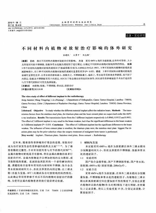
不同材料内植物对放射治疗影响的体外研究　宋建民　王勇平　刘志强　【摘要】　目的探讨不同材料内植物对放射治疗的影响。方法采用６ＭＶ－ｘ线作为放射源，在体外对形状、大小　及厚度相同的不锈钢板、钛板和骨水泥板的透射因子进行测定，以确定不同材料内植物对射线的阻挡情况。结果　３种不同材料内植物对射线的透射因子（衰减系数）分别为：０．８９６０，０．９５５２，０．９９５１，３种不同材料内植物对射线的衰　减影响很小，但３种不同材料内植物对射线的衰减有显著性差异（尸ｃ　Ｏ．０５）。结论３种不同材料内植物对射线的　衰减有显著性差异，以骨水泥的影响最小，钛板次之，不锈钢板最大，临床上，骨水泥常用来填充骨缺损，而不用于　内固定，钛板及不锈钢板常用于内固定，同时由于钛金属良好的组织相容性，因此恶性骨肿瘤保肢手术治疗选用骨　与关节替代材料时可优先选择钛板。　【关键词】内植物：钛板：不锈钢板；骨水泥；放射治疗　【中图分类号ｌ　Ｒ３１８．０８　【文献标识码ｌＡ　

Ｔｈｅ　ｖｉｔｒｏ　ｓｔｕｄｙ　ｏｆ　ｅｆｆｅｃｔ　ｏｆ　ｄｉｆｅｒｅｎｔ　ｉｍｐｌａｎｔ　ｔｏ　ｔｈｅ　ｒａｄｉｏｔｈｅｒａｐｙ　ＳｏｎｇＪｉａｎｍｉｎ１．Ｗａｎｇ　ＹｏｎｇｐｉｎｇＩ　ＬｉｕＺｈｉｑｉａｎｇ２，ｌ　ＤｅｐａｒｔｍｅｎｔｏｆＯｒｔｈｏｐｅｄｉｃｓ，Ｇａｎｓｕ　ＴｕｍｏｒＨｏｓｐｉｔａｌ，Ｌａｎｚｈｏｕ　７３００５０，　ＧａｎｓｕＰｒｏｖｉｎｃｅ，Ｃｈｉｎａ　２ＤｅｐａｒｔｍｅｎｔｏｆＲａｄｉａｔｉｏｎ　Ｏｎｃｏｌｏｇｙ，Ｇａｎｓｕ　ＴｕｍｏｒＨｏｓｐｉｔａｌ，Ｌａｎｚｈｏｕ　７３００５０，ＧａｎｓｕＰｒｏｖｉｎｃｅ，　Ｃｈｉｎａ　ＩＡｂｓｔｒａｃｔ】０ｂｊｅｅｔｉｖｅ　Ｔｏ　ｓｔｕｄｙ　ｗｈｅｔｈｅｒ　ｔｈｅ　ｄｉｆｅｒｅｎｔ　ｍａｔｅｒｉａｌ　ｉｍｐｌａｎｔ　ａｆｆｅｃｔ　ｔｈｅ　ｒａｄｉａｔｉｏｎ　ｂｅａｍ．Ｍｅｔｈｏｄｓ　Ｔｈｅ　ｔｒａｎｓ—　ｍｉｓｓｉｏｎ　ｆａｃｔｏｒｓ　ｆｒｏｍ　ｔｈｅ　ｓｔａｉｎｌｅｓｓ　ｓｔｅｅｌ　ｐｌａｔｅ．ｔＩｌｅ　ｔｉｔａｎｉｕｍ　ｐｌａｔｅ　ａｎｄ　ｔｈｅ　ｂｏｎｅ　ｃｅｍｅｎｔ　ｐｌａｔｅ　ａｒｅ　ｓｕｐｅｒｖｉｓｅｄ　ｕｎｄｅｒ　ｔｈｅ　６ＭＶ－　Ｘ　ｒａｙ　ｉｒｒａｄｉａｔｉｏｎ．Ｒｅｓｕｌｔｓ　Ｔｈｅ　ｔｒａｎｓｍｉｓｓｉｏｎ　ｆａｃｔｏｒ　ｆｒｏｍ　ｔｈｅ　３　ｄｉｆｅｒｅｎｔ　ｉｍｐｌａｎｔｓ　ｒｅｓｐｅｃｔｉｖｅｌｙ　ｉｓ　Ｏ．８９６０．Ｏ．９５５２　ａｎｄ　Ｏ．９９５　１．　Ｔｈｅ　ｅｆｆｅｃｔｏｆ３　ｄｉｆｆｅｒｅｎｔｉｍｐｌａｎｔｉｓｖｅｒｙ　ｓｍａｌｌｔｏｔｈｅｂｅａｍｗｅａｋｅｎ，ｂｕｔｉｔｈａｓｔｈｅ　ｓｉｇｎｉｆｉｃａｎｔｄｉｆｅｒｅｎｃｅｔｏｔｈｅｂｅａｍｗｅａｋｅｎ　ｉｎ３ｄｉｆｆｅｒｅｎｔｉｍｐｌａｎｔｓｆ／，＜Ｏ．０５）．Ｃｏｎｃｌｕｓｉｏｎ　Ｔｈｅｅｆｆｅｃｔｏｆ３　ｄｉｆｅｒｅｎｔｉｍｐｌａｎｔｈａｓｔｈｅ　ｓｉｇｎｉｆｉｃａｎｔｄｉｆｆｅｒｅｎｃｅｔｏｔｈｅｂｅａｍ　ｗｅａｋｅｎ．Ｔｈｅ　ｉｎｆｌｕｅｎｃｅ　ｏｆ　ｂｏｎｅ　ｃｅｍｅｎｔ　ｐｌａｔｅ　ｉｓ　ｓｍａｌｌｅｓｔ，ｔｈｅ　ｔｉｔａｎｉｕｍ　ｐｌａｔｅ　ｎｅｘｔ，ｔｈｅ　ｓｔａｉｎｌｅｓｓ　ｓｔｅｅｌ　ｐｌａｔｅ　ｂｉｇｇｅｓｔ．Ｔｈｅ　ｔｉｔ—　ａｎｉｕｍ　ｐｌａｔｅ　ｍａｙ　ｂｅ　ｔｈｅ　ｐｒｉｏｒ　ｓｅｌｅｃｔｉｏｎ　ｗｈｅｎ　ｔｈｅ　ｓｕｒｇｅｒｙ　ｔｒｅａｔｍｅｎｔ　ｏｆｍａｌｉｇｎａｎｔ　ｂｏｎｅ　ｔｕｍｏｒ　ｉｓ　ｐｅｒｆｏｒｍｅｄ．　ＩＫｅｙ　ｗｏｒｄｓＪ　Ｉｍｐｌａｎｔ；Ｔｉｔａｎｉｕｍ　ｐｌａｔｅ；Ｓｔａｉｎｌｅｓｓ　ｓｔｅｅｌ　ｐｌａｔｅ；Ｂｏｎｅ　ｃｅｍｅｎｔ；Ｒａｄｉｏｔｈｅｒａｐｙ　

近距离放射治疗

近距离放射治疗近距离放射治疗简史1898年居里夫妇宣布发现了一种称为镭的放射性物质。

1901年物理学家Becquera 在实验中意外受到镭的灼伤。

1903年由Goldberg等首先用镭盐管直接贴近皮肤表面治疗皮肤基底细胞癌，并取得了人们意想不到的疗效。

1913年镭首次用于宫颈癌的治疗。

1914年Failla收集了镭蜕变时释放的气体—氡，装入小型的容器中，植入瘤体做永久性植入，开始了组织间放射治疗。

1921年Sievert提出了点源、线源的剂量计算公式并一直延用至今。

由于近距离放疗时操作人员受量过大以及误认为外照射可以应付一切，使近距离放疗的应用受到一定的限制，主要只用于妇科肿瘤。

为了解决放射防护问题，自上世纪60年代初，在英国、瑞士……等国的几个医疗中心分别研制了“后装式”腔内放疗机，提出了后装技术。

上世纪80年代中期，应用程控步进马达驱动高活度微型放射源，辅以严谨的安全连锁系统的计算机控制后装机的出现，使近距离放疗技术得以迅速发展，扩展至全身多种肿瘤的治疗，它与外照射配合，体现了放疗发展的新趋势。

近距离放射治疗定义近距离放疗是指将封闭的放射源直接放置在人体内或体表需要治疗的部位进行放射治疗。

近距离放疗的特点放射源的强度较小，有效治疗距离短，射线能量大部分被组织吸收。

剂量分布遵循平方反比定律，它是近距离放射治疗剂量学最基本最重要的特点，即放射源周围的剂量分布，是按照与放射源之间距离的平方而下降。

在近距离照射条件下，平方反比定律是影响放射源周围剂量分布的主要因素，基本不受辐射能量的影响。

因此在治疗范围内，剂量不可能均匀，近源处剂量高，随距离增加剂量快速下降。

剂量率效应：根据参考点剂量率划分为低剂量率、中剂量率（4~12Gy/h）和高剂量率。

放射源近距离放射治疗使用放射性同位素源，除镭-226外，均为人工合成放射性同位素。

镭-226是天然放射性同位素，半衰期为1590年，先衰变为放射性气体氡，后者在衰变为稳定的同位素铅。

EPA 353.2

DETERMINATION OF NITRATE-NITRITE NITROGEN BY AUTOMATEDCOLORIMETRYEdited by James W. O'DellInorganic Chemistry BranchChemistry Research DivisionRevision 2.0August 1993ENVIRONMENTAL MONITORING SYSTEMS LABORATORYOFFICE OF RESEARCH AND DEVELOPMENTU.S. ENVIRONMENTAL PROTECTION AGENCYCINCINNATI, OHIO 45268353.2-1DETERMINATION OF NITRATE-NITRITE NITROGEN BY AUTOMATEDCOLORIMETRY1.0SCOPE AND APPLICATION1.1This method covers the determination of nitrite singly, or nitrite and nitratecombined in drinking, ground, surface, domestic and industrial wastes.1.2The applicable range is 0.05-10.0 mg/L nitrate-nitrite nitrogen. The range maybe extended with sample dilution.2.0SUMMARY OF METHOD2.1 A filtered sample is passed through a column containing granulated copper-cadmium to reduce nitrate to nitrite. The nitrite (that was originally presentplus reduced nitrate) is determined by diazotizing with sulfanilamide andcoupling with N-(1-naphthyl)-ethylenediamine dihydrochloride to form ahighly colored azo dye which is measured colorimetrically. Separate, ratherthan combined nitrate-nitrite, values are readily obtained by carrying out theprocedure first with, and then without, the Cu-Cd reduction step.2.2Reduced volume versions of this method that use the same reagents and molarratios are acceptable provided they meet the quality control and performancerequirements stated in the method.2.3Limited performance-based method modifications may be acceptable providedthey are fully documented and meet or exceed requirements expressed inSection 9.0, Quality Control.3.0DEFINITIONS3.1Calibration Blank (CB) -- A volume of reagent water fortified with the samematrix as the calibration standards, but without the analytes, internalstandards, or surrogate analytes.3.2Calibration Standard (CAL) -- A solution prepared from the primary dilutionstandard solution or stock standard solutions and the internal standards andsurrogate analytes. The CAL solutions are used to calibrate the instrumentresponse with respect to analyte concentration.3.3Instrument Performance Check Solution (IPC) -- A solution of one or moremethod analytes, surrogates, internal standards, or other test substances usedto evaluate the performance of the instrument system with respect to a definedset of criteria.353.2-23.4Laboratory Fortified Blank (LFB) -- An aliquot of reagent water or other blankmatrices to which known quantities of the method analytes are added in thelaboratory. The LFB is analyzed exactly like a sample, and its purpose is todetermine whether the methodology is in control, and whether the laboratoryis capable of making accurate and precise measurements.3.5Laboratory Fortified Sample Matrix (LFM) -- An aliquot of an environmentalsample to which known quantities of the method analytes are added in thelaboratory. The LFM is analyzed exactly like a sample, and its purpose is todetermine whether the sample matrix contributes bias to the analytical results.The background concentrations of the analytes in the sample matrix must bedetermined in a separate aliquot and the measured values in the LFMcorrected for background concentrations.3.6Laboratory Reagent Blank (LRB) -- An aliquot of reagent water or other blankmatrices that are treated exactly as a sample including exposure to allglassware, equipment, solvents, reagents, internal standards, and surrogatesthat are used with other samples. The LRB is used to determine if methodanalytes or other interferences are present in the laboratory environment, thereagents, or the apparatus.3.7Linear Calibration Range (LCR) -- The concentration range over which theinstrument response is linear.3.8Material Safety Data Sheet (MSDS) -- Written information provided byvendors concerning a chemical's toxicity, health hazards, physical properties,fire, and reactivity data including storage, spill, and handling precautions.3.9Method Detection Limit (MDL) -- The minimum concentration of an analytethat can be identified, measured and reported with 99% confidence that theanalyte concentration is greater than zero.3.10Quality Control Sample (QCS) -- A solution of method analytes of knownconcentrations that is used to fortify an aliquot of LRB or sample matrix. TheQCS is obtained from a source external to the laboratory and different fromthe source of calibration standards. It is used to check laboratory performancewith externally prepared test materials.3.11Stock Standard Solution (SSS) -- A concentrated solution containing one ormore method analytes prepared in the laboratory using assayed referencematerials or purchased from a reputable commercial source.4.0INTERFERENCES4.1Build up of suspended matter in the reduction column will restrict sampleflow. Since nitrate and nitrite are found in a soluble state, samples may bepre-filtered.353.2-34.2Low results might be obtained for samples that contain high concentrations ofiron, copper or other metals. EDTA is added to the samples to eliminate thisinterference.4.3Residual chlorine can produce a negative interference by limiting reductionefficiency. Before analysis, samples should be checked and if required,dechlorinated with sodium thiosulfate.4.4Samples that contain large concentrations of oil and grease will coat thesurface of the cadmium. This interference is eliminated by pre-extracting thesample with an organic solvent.4.5Method interferences may be caused by contaminants in the reagent water,reagents, glassware, and other sample processing apparatus that bias analyteresponse.5.0SAFETY5.1The toxicity or carcinogenicity of each reagent used in this method have notbeen fully established. Each chemical should be regarded as a potential healthhazard and exposure should be as low as reasonably achievable. Cautions areincluded for known extremely hazardous materials or procedures.5.2Each laboratory is responsible for maintaining a current awareness file ofOSHA regulations regarding the safe handling of the chemicals specified inthis method. A reference file of Material Safety Data Sheets (MSDS) should bemade available to all personnel involved in the chemical analysis. Thepreparation of a formal safety plan is also advisable.5.3The following chemicals have the potential to be highly toxic or hazardous,consult MSDS.5.3.1Cadmium (Section 7.1)5.3.2Phosphoric acid (Section 7.5)5.3.3Hydrochloric acid (Section 7.6)5.3.4Sulfuric acid (Section 7.8)5.3.5Chloroform (Sections 7.10 and 7.11)6.0EQUIPMENT AND SUPPLIES6.1Balance -- Analytical, capable of accurately weighing to the nearest 0.0001 g.6.2Glassware -- Class A volumetric flasks and pipets as required.353.2-46.3Automated continuous flow analysis equipment designed to deliver and reactsample and reagents in the required order and ratios.6.3.1Sampling device (sampler)6.3.2Multichannel pump6.3.3Reaction unit or manifold6.3.4Colorimetric detector6.3.5Data recording device7.0REAGENTS AND STANDARDS7.1Granulated cadmium: 40-60 mesh (CASRN 7440-43-9). Other mesh sizes maybe used.7.2Copper-cadmium: The cadmium granules (new or used) are cleaned withdilute HCl (Section 7.6) and copperized with 2% solution of copper sulfate(Section 7.7) in the following manner:7.2.1Wash the cadmium with HCl (Section 7.6) and rinse with distilledwater. The color of the cadmium so treated should be silver.7.2.2Swirl 10 g cadmium in 100 mL portions of 2% solution of coppersulfate (Section 7.7) for five minutes or until blue color partially fades,decant and repeat with fresh copper sulfate until a brown colloidalprecipitate forms.7.2.3Wash the copper-cadmium with reagent water (at least 10 times) toremove all the precipitated copper. The color of the cadmium sotreated should be black.7.3Preparation of reduction column. The reduction column is a U-shaped, 35 cmlength, 2 mm I.D. glass tube (Note 1). Fill the reduction column with distilledwater to prevent entrapment of air bubbles during the filling operations.Transfer the copper-cadmium granules (Section 7.2) to the reduction columnand place a glass wool plug in each end. To prevent entrapment of airbubbles in the reduction column, be sure that all pump tubes are filled withreagents before putting the column into the analytical system.Note: Other reduction tube configurations, including a 0.081 I.D. pump tube,can be used in place of the 2 mm glass tube, if checked as in Section 10.1.7.4Reagent water: Because of possible contamination, this should be prepared bypassage through an ion exchange column comprised of a mixture of bothstrongly acidic-cation and strongly basic-anion exchange resins. The353.2-5regeneration of the ion exchange column should be carried out according tothe manufacturer's instructions.7.5Color reagent: To approximately 800 mL of reagent water, add, while stirring,100 mL conc. phosphoric acid (CASRN 7664-38-2), 40 g sulfanilamide (CASRN63-74-1) and 2 g N-1-naphthylethylenediamine dihydrochloride (CASRN 1465-25-4). Stir until dissolved and dilute to 1 L. Store in brown bottle and keep inthe dark when not in use. This solution is stable for several months.7.6Dilute hydrochloric acid, 6N: Add 50 mL of conc. HCl (CASRN 7647-01-0) toreagent water, cool, and dilute to 100 mL.7.7Copper sulfate solution, 2%: Dissolve 20 g of CuSO5H O (CASRN 7758-99-8)42in 500 mL of reagent water and dilute to 1 L.7.8Wash solution: Use reagent water for unpreserved samples. For samplespreserved with H SO, use 2 mL H SO (CASRN 7764-93-9), per liter of wash2424water.7.9Ammonium chloride-EDTA solution: Dissolve 85 g of reagent gradeammonium chloride (CASRN 12125-02-9) and 0.1 g of disodiumethylenediamine tetracetate (CASRN 6381-92-6) in 900 mL of reagent water.Adjust the pH to 9.1 for preserved or 8.5 for non-preserved samples with conc.ammonium hydroxide (CASRN 1336-21-6) and dilute to 1 L. Add 0.5 mL Brij-35 (CASRN 9002-92-0).7.10Stock nitrate solution: Dissolve 7.218 g KNO (CASRN 7757-79-1) and dilute to31 L in a volumetric flask with reagent water. Preserve with2 mL ofchloroform (CASRN 67-66-3) per liter. Solution is stable for six months. 1 mL= 1.0 mg NO-N.37.11Stock nitrite solution: Dissolve 6.072 g KNO in 500 mL of reagent water and2dilute to 1 L in a volumetric flask. Preserve with 2 mL of chloroform and keepunder refrigeration. 1.0 mL = 1.0 mg NO-N.27.12Standard nitrate solution: Dilute 1.0 mL of stock nitrate solution (Section 7.10)to 100 mL. 1.0 mL = 0.01 mg NO-N. Preserve with .2 mL of chloroform.3Solution is stable for six months.7.13Standard nitrite solution: Dilute 10.0 mL of stock nitrite (Section 7.11) solutionto 1000 mL. 1.0 mL = 0.01 mg NO-N. Solution is unstable; prepare as2required.8.0SAMPLE COLLECTION, PRESERVATION AND STORAGE8.1Samples should be collected in plastic or glass bottles. All bottles must bethoroughly cleaned and rinsed with reagent water. Volume collected should353.2-6be sufficient to insure a representative sample, allow for replicate analysis (ifrequired), and minimize waste disposal.8.2Samples must be preserved with H SO to a pH <2 and cooled to 4°C at the24time of collection.8.3Samples should be analyzed as soon as possible after collection. If storage isrequired, preserved samples are maintained at 4°C and may be held for up to28 days.8.4Samples to be analyzed for nitrate or nitrite only should be cooled to 4°C andanalyzed within 48 hours.9.0QUALITY CONTROL9.1Each laboratory using this method is required to operate a formal qualitycontrol (QC) program. The minimum requirements of this program consist ofan initial demonstration of laboratory capability and the periodic analysis oflaboratory reagent blanks, fortified blanks, and other laboratory solutions as acontinuing check on performance. The laboratory is required to maintainperformance records that define the quality of the data that are generated.9.2INITIAL DEMONSTRATION OF PERFORMANCE9.2.1The initial demonstration of performance is used to characterizeinstrument performance (determination of LCR and analysis of QCS)and laboratory performance (determination of MDLs) prior toperforming analyses by this method.9.2.2Linear Calibration Range (LCR) -- The LCR must be determinedinitially and verified every six months or whenever a significant changein instrument response is observed or expected. The initialdemonstration of linearity must use sufficient standards to insure thatthe resulting curve is linear. The verification of linearity must use aminimum of a blank and three standards. If any verification dataexceeds the initial values by ±10%, linearity must be reestablished. Ifany portion of the range is shown to be nonlinear, sufficient standardsmust be used to clearly define the nonlinear portion.9.2.3Quality Control Sample (QCS) -- When beginning the use of thismethod, on a quarterly basis or as required to meet data-quality needs,verify the calibration standards and acceptable instrument performancewith the preparation and analyses of a QCS. If the determinedconcentrations are not within ±10% of the stated values, performance ofthe determinative step of the method is unacceptable. The source ofthe problem must be identified and corrected before either proceedingwith the initial determination of MDLs or continuing with on-goinganalyses.353.2-79.2.4Method Detection Limit (MDL) -- MDLs must be established for allanalytes, using reagent water (blank) fortified at a concentration of two(6)to three times the estimated instrument detection limit. To determineMDL values, take seven replicate aliquots of the fortified reagent waterand process through the entire analytical method. Perform allcalculations defined in the method and report the concentration valuesin the appropriate units. Calculate the MDL as follows:where,t =Student's t value for a 99% confidence level and astandad deviation estimate with n-1 degrees offreedom [t = 3.14 for seven replicates]S = standard deviation of the replicate analyses MDLs should be determined every six months, when a new operatorbegins work, or whenever there is a significant change in thebackground or instrument response.9.3ASSESSING LABORATORY PERFORMANCE9.3.1Laboratory Reagent Blank (LRB) -- The laboratory must analyze at leastone LRB with each batch of samples. Data produced are used to assesscontamination from the laboratory environment. Values that exceed theMDL indicate laboratory or reagent contamination should be suspectedand corrective actions must be taken before continuing the analysis.9.3.2Laboratory Fortified Blank (LFB) -- The laboratory must analyze at leastone LFB with each batch of samples. Calculate accuracy as percentrecovery (Section 9.4.2). If the recovery of any analyte falls outside therequired control limits of 90-110%, that analyte is judged out of control,and the source of the problem should be identified and resolved beforecontinuing analyses.9.3.3The laboratory must use LFB analyses data to assess laboratoryperformance against the required control limits of 90-110%. Whensufficient internal performance data become available (usually aminimum of 20-30 analyses), optional control limits can be developedfrom the percent mean recovery (x) and the standard deviation (S) ofthe mean recovery. These data can be used to establish the upper andlower control limits as follows:UPPER CONTROL LIMIT = x + 3SLOWER CONTROL LIMIT = x - 3SThe optional control limits must be equal to or better than the requiredcontrol limits of 90-110%. After each five to ten new recoverymeasurements, new control limits can be calculated using only the mostrecent 20-30 data points. Also, the standard deviation (S) data shouldbe used to established an on-going precision statement for the level ofconcentrations included in the LFB. These data must be kept on fileand be available for review.9.3.4Instrument Performance Check Solution (IPC) -- For all determinationsthe laboratory must analyze the IPC (a mid-range check standard) anda calibration blank immediately following daily calibration, after every10th sample (or more frequently, if required), and at the end of thesample run. Analysis of the IPC solution and calibration blankimmediately following calibration must verify that the instrument iswithin ±10% of calibration. Subsequent analyses of the IPC solutionmust verify the calibration is still within ±10%. If the calibration cannotbe verified within the specified limits, reanalyze the IPC solution. If thesecond analysis of the IPC solution confirms calibration to be outsidethe limits, sample analysis must be discontinued, the cause determinedand/or in the case of drift, the instrument recalibrated. All samplesfollowing the last acceptable IPC solution must be reanalyzed. Theanalysis data of the calibration blank and IPC solution must be kept onfile with the sample analyses data.9.4ASSESSING ANALYTE RECOVERY AND DATA QUALITY9.4.1Laboratory Fortified Sample Matrix (LFM) -- The laboratory must add aknown amount of analyte to a minimum of 10% of the routine samples.In each case, the LFM aliquot must be a duplicate of the aliquot usedfor sample analysis. The analyte concentration must be high enough tobe detected above the original sample and should not be less than fourtimes the MDL. The added analyte concentration should be the sameas that used in the laboratory fortified blank.9.4.2Calculate the percent recovery for each analyte, corrected forconcentrations measured in the unfortified sample, and compare thesevalues to the designated LFM recovery range 90-110%. Percentrecovery may be calculate using the following equation:where,R =percent recoveryC =fortified sample concentrationsC = sample background concentrations = concentration equivalent of analyte added tosample9.4.3If the recovery of any analyte falls outside the designated LFM recoveryrange and the laboratory performance for that analyte is shown to be incontrol (Section 9.3), the recovery problem encountered with the LFM isjudged to be either matrix or solution related, not system related.9.4.4Where reference materials are available, they should be analyzed toprovide additional performance data. The analysis of reference samplesis a valuable tool for demonstrating the ability to perform the methodacceptably.10.0CALIBRATION AND STANDARDIZATION10.1Prepare a series of at least three standards, covering the desired range, and ablank by diluting suitable volumes of standard nitrate solution (Section 7.12).At least one nitrite standard should be compared to a nitrate standard at thesame concentration to verify the efficiency of the reduction column.10.2Set up manifold as shown in Figure 1. Care should be taken not to introduceair into the reduction column.10.3Place appropriate standards in the sampler in order of decreasingconcentration and perform analysis.10.4Prepare standard curve by plotting instrument response against concentrationvalues. A calibration curve may be fitted to the calibration solutionsconcentration/response data using computer or calculator based regressioncurve fitting techniques. Acceptance or control limits should be establishedusing the difference between the measured value of the calibration solutionand the "true value" concentration.10.5After the calibration has been established, it must be verified by the analysis ofa suitable quality control sample (QCS). If measurements exceed ±10% of theestablished QCS value, the analysis should be terminated and the instrumentrecalibrated. The new calibration must be verified before continuing analysis.Periodic reanalysis of the QCS is recommended as a continuing calibrationcheck.Note: Condition column by running 1 mg/L standard for 10 minutes if a newreduction column is being used. Subsequently wash the column with reagentsfor 20 minutes.11.0PROCEDURE11.1If the pH of the sample is below 5 or above 9, adjust to between 5 and 9 witheither conc. HCl or conc. NH OH.411.2Set up the manifold as shown in Figure 1. Care should be taken not tointroduce air into reduction column.11.3Allow system to equilibrate as required. Obtain a stable baseline with allreagents, feeding reagent water through the sample line.11.4Place appropriate nitrate and/or nitrite standards in sampler in order ofdecreasing concentration and complete loading of sampler tray.11.5Switch sample line to sampler and start analysis.12.0DATA ANALYSIS AND CALCULATIONS12.l Prepare a calibration curve by plotting instrument response against standardconcentration. Compute sample concentration by comparing sample responsewith the standard curve. Multiply answer by appropriate dilution factor.12.2Report only those values that fall between the lowest and the highestcalibration standards. Samples exceeding the highest standard should bediluted and reanalyzed.l2.3Report results in mg/L as nitrogen.13.0METHOD PERFORMANCE13.1Three laboratories participating in an EPA Method Study analyzed four naturalwater samples containing exact increments of inorganic nitrate, with thefollowing results:Increment as Precision as Accuracy asNitrate Nitrogen Standard Deviation Bias, Bias,mg N/L mg N/L % mg N/L0.290.012+ 5.75+ 0.0170.350.092+ 18.10+ 0.0632.310.318+ 4.47+ 0.1032.480.176- 2.69- 0.06713.2The interlaboratory precision and accuracy data in Table 1 were developedusing a reagent water matrix. Values are in mg NO-N/L.313.3Single laboratory precision data can be estimated at 50-75% of theinterlaboratory precision estimates.l4.0POLLUTION PREVENTION14.1Pollution prevention encompasses any technique that reduces or eliminates thequantity or toxicity of waste at the point of generation. Numerousopportunities for pollution prevention exist in laboratory operation. The EPAhas established a preferred hierarchy of environmental management techniquesthat places pollution prevention as the management option of first choice.Whenever feasible, laboratory personnel should use pollution preventiontechniques to address their waste generation. When wastes cannot be feasiblyreduced at the source, the Agency recommends recycling as the next bestoption.14.2The quantity of chemicals purchased should be based on expected usageduring its shelf life and disposal cost of unused material. Actual reagentpreparation volumes should reflect anticipated usage and reagent stability.14.3For information about pollution prevention that may be applicable tolaboratories and research institutions, consult "Less is Better: LaboratoryChemical Management for Waste Reduction", available from the AmericanChemical Society's Department of Government Regulations and Science Policy,1155 16th Street N.W., Washington, D.C. 20036, (202) 872-4477.15.0WASTE MANAGEMENT15.1The Environmental Protection Agency requires that laboratory wastemanagement practices be conducted consistent with all applicable rules andregulations. Excess reagents, samples, and method process wastes should becharacterized and disposed of in an acceptable manner. The Agency urgeslaboratories to protect the air, water, and land by minimizing and controllingall releases from hoods and bench operations, complying with the letter andspirit of any waste discharge permit and regulations, and by complying withall solid and hazardous waste regulations, particularly the hazardous wasteidentification rules and land disposal restrictions. For further information onwaste management consult the "Waste Management Manual for LaboratoryPersonnel", available from the American Chemical Society at the address listedin Section 14.3.16.0REFERENCES1.Fiore, J., and O'Brien, J.E., "Automation in Sanitary Chemistry - Parts 1 & 2:Determination of Nitrates and Nitrites", Wastes Engineering 33, 128 &238(1962).2.Armstrong, F.A., Stearns, C.R., and Strickland, J.D., "The Measurement ofUpwelling and Subsequent Biological Processes by Means of the TechniconAutoAnalyzer and Associated Equipment", Deep Sea Research 14, pp. 381-389(1967).3.Annual Book of ASTM Standards, Part 31, "Water", Standard D1254, p. 366(1976).4.Standard Methods for the Examination of Water and Wastewater, 17th Edition,pp. 4-91, Method 4500-NO3 F (1992).5.Chemical Analyses for Water Quality Manual, Department of the Interior,FWPCA, R.A. Taft Engineering Center Training Program, Cincinnati, Ohio45226 (January, 1966).6.Code of Federal Regulations 40, Ch. 1, Pt. 136, Appendix B.17.0TABLES, DIAGRAMS, FLOWCHARTS AND VALIDATION DATATABLE 1. INTERLABORATORY PRECISION AND ACCURACY DATA Number of True StandardValues Value Mean Residual Deviation ResidualReported(T)(X)for X(S)for S 1630.2500.24790.00070.0200-0.00011830.4510.4441-0.00390.0289-0.00022130.6500.64790.00120.03980.00171700.9500.95370.00740.0484-0.0031163 1.90 1.89870.00370.0918-0.0024172 2.20 2.19710.00250.11640.0087183 2.41 2.3732-0.03120.12730.0102214 3.20 3.20420.01090.1456-0.0070172 6.50 6.49780.00890.31560.01482138.007.9814-0.00550.3673-0.00081708.508.51350.02730.3635-0.027121410.09.9736-0.01060.4353-0.0227 REGRESSIONS: X = 0.999T + 0.002, S = 0.045T + 0.009。

谱分析和结构信息：烟灰和相关含碳材料的显微拉曼散射光谱

Raman microspectroscopy of soot and relatedcarbonaceous materials:Spectral analysis and structural informationA.Sadezkya,1,H.Muckenhuber b ,H.Grothe b ,R.Niessner a ,U.Po ¨schla,*a Institute of Hydrochemistry,Technical University of Munich,Marchioninistr.17,D-81377Munich,GermanybInstitute of Materials Chemistry,Vienna University of Technology,Veterinaerplatz 1/GA,A-1210Vienna,AustriaReceived 6September 2004;accepted 10February 2005Available online 23March 2005AbstractExperimental conditions and mathematical ﬁtting procedures for the collection and analysis of Raman spectra of soot and related carbonaceous materials have been investigated and optimised with a Raman microscope system operated at three diﬀerent laser excitation wavelengths (514,633,and 780nm).Several band combinations for spectral analysis have been tested,and a com-bination of four Lorentzian-shaped bands (G,D1,D2,D4)at about 1580,1350,1620,and 1200cm À1,respectively,with a Gaussian-shaped band (D3)at $1500cm À1was best suited for the ﬁrst-order spectra.The second-order spectra were best ﬁtted with Lorentz-ian-shaped bands at about 2450,2700,2900,and 3100cm À1.Spectral parameters (band positions,full widths at half maximum,and intensity ratios)are reported for several types of industrial carbon black (Degussa Printex,Cabot Monarch),diesel soot (particulate matter from modern heavy duty vehicle and passenger car engine exhaust,NIST SRM1650),spark-discharge soot (Palas GfG100),and graphite.Several parameters,in particular the width of the D1band at $1350cm À1,provide structural information and allow to discriminate the sample materials,but the characterisation and distinction of diﬀerent types of soot is limited by the experimental reproducibility of the spectra and the statistical uncertainties of curve ﬁtting.The results are discussed and compared with X-ray diﬀraction measurements and earlier Raman spectroscopic studies of comparable materials,where diﬀerent measurement and ﬁtting procedures had been applied.Ó2005Elsevier Ltd.All rights reserved.Keywords:Soot,Graphitic carbon;Raman spectroscopy;Microstructure1.IntroductionSoot is technically deﬁned as the black solid product of incomplete combustion or pyrolysis of fossil fuels and other organic materials.It plays important roles as an industrial ﬁller and pigment on the one hand (carbon black),and as a traﬃc-related air pollutant on the other hand (diesel soot).Soot is primarily composed of carbon (>80%)and consists of agglomerated primary particleswith diameters on the order of 10–30nm comprising crystalline and amorphous domains.The graphite-like crystalline domains typically consist of 3–4turbostrati-cally stacked graphene layers,with average lateral exten-sions (L a )of up to $3nm and interlayer distances ofabout 3.5A˚,and can be regarded as highly disordered graphitic lattices [1,2].In an ideal graphitic lattice the distance between parallel graphene layers (planar hexag-onal structures of sp 2-hybridized carbon atoms withcovalent bond lengths of 1.42A˚)is 3.35A ˚,and the lay-ers are arranged in an alternating sequence ABAB.This corresponds to a hexagonal closest crystal structure with unit cells of four C atoms at two types of lattice sites with diﬀerent coordination (two or no neighbouring C atoms on a perpendicular axis through the adjacent0008-6223/$-see front matter Ó2005Elsevier Ltd.All rights reserved.doi:10.1016/j.carbon.2005.02.018*Corresponding author.Tel.:+49218078238;fax:+4989218078255.E-mail address:ulrich.poeschl@ch.tum.de (U.Po ¨schl).1Now at Laboratoire de Combustion et de Systemes Reactifs,CNRS,F-45071Orleans,France.Carbon 43(2005)1731–1742/locate/carbonparallel layers).The amorphous(i.e.non-graphite-like) domains are composed of polycyclic aromatic com-pounds,which can be regarded as graphene layer pre-cursors in irregular or onion-like arrangements (fullerenoid structures),and other organic and inorganic components(aliphatics,sulfate,metal oxides,etc.).The actual physical and chemical structure of soot,its ele-mental composition(carbon,hydrogen,oxygen,etc.), and the ratio of crystalline graphite-like to amorphous organic carbon depend on the starting materials and conditions of the combustion or pyrolysis process(fuel type,fuel/oxygen ratio,ﬂame temperature,residence time,etc.[2,3])The graphitic carbon fraction of soot can be increased by annealing procedures at high tem-peratures[2–5].For the structural characterisation of highly ordered solid materials(crystalline long-range order)diﬀraction techniques are usually the methods of choice.For highly disordered materials such as soot,however,Raman spectroscopy is more promising,because it is sensitive not only to crystal structures but also to molecular structures(short-range order).The Raman signals of graphite crystals result from lattice vibrations and are very sensitive to the degree of structural disorder.The spectrum of near-ideal graphite,which is observed for large single graphitic crystals and highly oriented poly-crystalline graphite(HOPG),signiﬁcantly diﬀers from the Raman spectra of disturbed graphitic lattices,such as regular polycrystalline graphite or boron-doted HOPG[6–17](Table1).Among the substances investi-gated in earlier studies are diﬀerent types of graphite [6,12,13,17–19],diamondﬁlms[15,20],glassy carbon [18,19,21],amorphous and graphitic carbonﬁlms [4,22],coal,pitch and coalﬁbres[18],activated carbon [18,19],and fullerenes[23].Rosen and Novakov [24,25]haveﬁrst used Raman spectroscopy to prove the presence of graphite-like carbon in diesel engine soot,and their investigations have been followed up in several other studies[3,5,13,22,26,27].Some of these studies found that diﬀerent types of soot could be distin-guished according to their degree of graphitisation [3,5,13,18,19,26].In the acquisition,analysis,and inter-pretation of the broad and overlapping Raman bands of soot,however,a wide range of diﬀerent approaches has been followed.The spectral parameters correlated to the degree of graphitisation have been determined in diﬀerent ways,which makes the results hard to com-pare and limits their conclusiveness.Thus we have set out to investigate the applicability of Raman micro-spectroscopy for the structural characterisation of soot by systematic experiments and spectral analyses.Raman spectra have been recorded for a wide variety of soot and related materials(diesel soot,spark discharge soot, industrial carbon black,graphite,polycyclic aromatic hydrocarbons)under varying measurement conditions using a Raman microscope system with three diﬀerent excitation wavelengths(k0).The Raman spectra have been analysed by curveﬁtting with diﬀerent band com-binations,and the obtained spectral parameters and their structural information are discussed in view of the results of earlier studies.2.Experimental2.1.SamplesEight diﬀerent types of industrial soot(carbon black) were available as powder samples(Degussa:S160,Prin-tex140U,Printex25,Printex60,Printex75,Printex90, and Printex XE2;Cabot:Monarch77,Monarch120). Spark discharge soot was taken from a glassﬂask at the outlet of a Palas GfG1000aerosol generator(pow-der sample).Diesel soot was available as a standard reference material(SRM1650,NIST;powder sample)and in the form of polycarbonate and glassﬁbreﬁlter samples collected from the exhaust of modern diesel engines(ATable1First-order Raman bands and vibration modes reported for soot and graphite(vs=very strong,s=strong,m=medium,w=weak)Band a Raman shift(cmÀ1)Vibration mode bSoot Disordered graphite c Highly ordered graphite dG$1580cmÀ1,s$1580cmÀ1,s$1580cmÀ1,s Ideal graphitic lattice(E2g-symmetry)[6,17]D1(D)$1350cmÀ1,vs$1350cmÀ1,m–Disordered graphitic lattice(graphene layer edges,A1g symmetry)[6,17]D2(D0)$1620cmÀ1,s$1620cmÀ1,w–Disordered graphitic lattice(surface graphene layers,E2g-symmetry)[17]D3(D00,A)$1500cmÀ1,m––Amorphous carbon(Gaussian[26]or Lorentzian[3,18,27]line shape)D4(I)$1200cmÀ1,w––Disordered graphitic lattice(A1g symmetry)[10],polyenes[3,27],ionic impurities[18]a Alternative band designations of earlier studies are given in brackets.b Lorentzian line shape unless mentioned otherwise.c Polycrystalline graphite(<100nm)and boron-doted HOPG[17].d Single graphitic crystals(>100nm)and HOPG[17].1732 A.Sadezky et al./Carbon43(2005)1731–1742and B:heavy-duty vehicles;C and D:passenger cars). Graphite was investigated in the form of a solid elec-trode bar as used in the spark discharge generator (99.9995%,Johnston-Matthey)and in the form of pow-der samples(SHER graphite,<100l m,Heraeus;syn-thetic graphite,1–2l m,Aldrich).The polycyclic aromatic hydrocarbon hexa-benzo-coronene(HBC) was synthesized and supplied by the research group of K.Mu¨llen(Max Planck Institute for Polymer Research, Mainz,Germany).2.2.X-ray diﬀractionThe investigated soot and graphite powder samples were placed on the sample support(silicon)of the X-ray diﬀractometer(Philips XÕpert PW3050/60)and illu-minated with Ni-ﬁltered copper radiation(Cu K a1: k1=1.54051A˚;K a2:k2=1.54433A˚).The diﬀraction pattern was recorded at room temperature in the2H range from10to60°(resolution0.02°,counting time 5s per interval).2.3.Raman measurement and spectral analysisThe applied Raman microscope systems(Renishaw, System2000;Yobin Yvon,LabRAM HR)consisted of a light microscope(Leica DL-LM;Olympus BX)cou-pled to a Raman spectrometer with three diﬀerent exci-tation lasers.The microscope was equipped with four objectives with5·,20·,50·,and100·magniﬁcation, respectively,and with an eyepiece with10·magniﬁca-tion.The microscope optics were used to focus the excitation laser beam onto the sample and to collect the backscattered light(180°).The Rayleigh scattering component was removed by a Notchﬁlter,and the Raman-scattered light was dispersed by an optical grid and detected by a CCD camera(maximum sensitivity at500–850nm wavelength).The excitation lasers were an Ar ion laser(k0=514nm,source power17mW),a He–Ne laser(k0=632.8nm,source power25mW), and a NIR diode laser(k0=780nm,source power 26mW).The laser beam power was adjustable from 1%to100%of the source power.The diameter of the laser spot on the sample surface was1l m for the fully focused laser beam,and40l m for the fully defocused laser beam at50·objective magniﬁcation.The spectral resolution was about6cmÀ1at514nm,4cmÀ1at633 nm,and2cmÀ1at780nm.The instrument was cali-brated against the Stokes Raman signal of pure Si at 520cmÀ1using a silicon wafer((111)crystal plane sur-face).Instrument control and spectral analysis were per-formed with the software packages Renishaw WiRE (Renishaw)and GRAMS/32(Galactic).For the powder samples,a dense layer of about one millimeter thickness was pressed with a steel spatula onto a silicon wafer (macroscopically smooth surface)and placed on the microscope sample holder;ﬁlter samples and the graph-ite bar were placed directly on the sample holder.The microscope was focused onto the sample surface using the white light source and the objective with50·magni-ﬁcation.Then the white light was replaced by the laser beam and Raman spectra were recorded(Stokes Raman shift500–4000cmÀ1).The Raman spectrometer was generally operated in the continuous scanning mode. The power of the excitation laser beam(1–100%relative intensity),spot diameter(0–100%defocusing),and exposure time have been varied toﬁnd optimum mea-surement conditions.For soot samples spectra of high-est quality and reproducibility were generally obtained with fully defocused laser beam,laser beam powers of 10%(514nm)to100%(780nm),and exposure times of at least120s.For graphite samples,on the other hand,best results were generally obtained with100% of the laser source power and fully focused laser beam, and exposure times of at least10s.Depending on the sample type and excitation wavelength,modiﬁed mea-surement conditions also yielded high quality spectra (e.g.100%laser power and25%defocusing for soot with k0=633nm).Curveﬁtting for the determination of spectral para-meters was performed with the software program GRAMS/32(Galactic,Levenberg–Marquardt algo-rithm).The goodness-of-ﬁt was indicated by the reduced v2value,which would be unity for perfect agreement be-tween the calculatedﬁt curve and the observed spectrum. Values between1and3imply that the curveﬁt converges towards the observed spectrum;values larger than3indi-cate that the iteration has reached a minimum,but does not converge[28].First-and second-order spectra were ﬁtted separately withoutﬁxing or limiting the range of any spectral parameter in the iteration procedure.Dif-ferent combinations ofﬁrst-order Raman bands andTable2Band combinations tested for curveﬁtting ofﬁrst-order Raman spectra of soot in this work and in earlier studies(initial band positions;line shapes: L=Lorentzian,G=Gaussian)Band Initial position(cmÀ1)(I)[18](II)[26](III)(IV)[19](V)[3,27](VI)(VII)(VIII)(IX)G1580L L L L L L L L LD11360L L L L L L L L LD21620–––L––L L LD31500L G––L G–L GD41180––L–L L L L LA.Sadezky et al./Carbon43(2005)1731–17421733their initial positions tested in this study are listed in Table2.3.Results and discussion3.1.X-ray diﬀractogramsThe diﬀraction pattern of the synthetic graphite sam-ple exhibits four distinctive narrow reﬂections in the2H range10–60°,which can be indicated as follows:26.8°(002layer),42.3°(100),44.5°(101)and54.9°(102). In contrast,the investigated soot samples show only two broad reﬂections with intensity maxima at24.9°and43.6°(Printex XE2)and at24.2°and43.4°(Printex 90),respectively(Fig.1).In the diﬀractogram of Printex90an additional nar-row signal appears at42.9°(marked by*);this is not due to the carbonaceous material but can be attributed to acontamination with tungsten carbide.Curveﬁtting yields the full width at half maximum(FWHM)of these reﬂexes,and the Debye-Scherrer formula can be used to estimate the average size of the crystallites or graphite-like crystalline domains contained in the samples[29]. These were250nm for the synthetic graphite,4nm for Printex XE2,and only2nm for Printex90.These values indicate a higher degree of order and graphitisation for Printex XE2compared to Printex90,which is consistent with the Raman spectroscopic results discussed below.3.2.Raman spectra of graphiteThe spectrum of the SHER graphite sample(Fig.2)is characteristic of an undisturbed graphitic lattice and exhibits only oneﬁrst-order band,the G(‘‘Graphite’’) band at around1580cmÀ1corresponding to an ideal graphitic lattice vibration mode with E2g symmetry.Such spectra are generally observed for highly ori-ented polycrystalline graphite(HOPG),and for single graphitic crystals,whose edge length L a parallel to the graphene layers is larger than100nm.The spectrum of the graphite bar,on the other hand,exhibits addi-tionalﬁrst-order bands(D or‘‘Defect’’bands),which are known to be characteristic for disordered graphite and to grow in intensity relative to the G band with increasing degree of disorder in the graphitic structure. The most intensive of them is the D1band,which appears at$1360cmÀ1and corresponds to a graphitic lattice vibration mode with A1g symmetry.Another ﬁrst-order band accounting for structural disorder is the D2band at$1620cmÀ1which can be observed as a shoulder on the G band.Like the G band,the D2 band corresponds to a graphitic lattice mode with E2g symmetry[9,10,18].The relative intensities of both the D1and D2bands increased with increasing k0(Fig.3), which can be attributed to resonance eﬀects[30].Spectra similar to that of the graphite bar have been observed for HOPG doted with0.5mol%of boron[17] Fig.1.X-ray diﬀractograms of graphite,Printex90,and Printex XE2.1734 A.Sadezky et al./Carbon43(2005)1731–1742or polycrystalline graphites with L a smaller than1000A˚[6,8–16,21].Theoretical calculations have shown that each of theﬁrst-order Raman bands visible in spectra of highly ordered and disordered graphites can be attrib-uted to a vibrational mode of the ideal graphitic lattice [8,10].For an ideal graphitic crystal(space group D46h with unlimited translational symmetry)only a few of these vibrational modes are Raman active.In case of structural disorders,however,some ideally forbidden vibrational modes can become Raman active.The D1 band has been suggested to arise from graphene layer carbon atoms in immediate vicinity of a lattice distur-bance like the edge of a graphene layer[14,17]or a het-eroatom in case of doted graphite[17].Moreover,this band has been observed in Raman spectra taken directly on the edge planes perpendicular to the graphene layers of large graphite single crystals and HOPG[14,17]. Thus,in polycrystalline carbonaceous materials consist-ing of large numbers of small graphitic crystallites car-bon atoms at the edge of graphene layers are considered as the most probable origin of the D band [14,17].The D2band was assigned to a lattice vibration analogous to that of the G band but involving graphene layers at the surface of a graphitic crystal[31],i.e.graph-ene layers which are not directly sandwiched between two other graphene layers.Indeed,the D2band was ob-served to replace the G band in intercalation compounds [9].In polycrystalline graphitic materials it can be re-garded as an indicator for the surface to volume ratio of graphitic crystals[19].For both samples the Raman spectra recorded with k0=514nm exhibited second-order bands at about2450,2720,and3240cmÀ1.The band at2720cmÀ1is the most intensive one and can be attributed to theﬁrst overtone of the D1band, (2*D1)[17,18].The spectrum of the SHER graphite exhibits a split of the(2*D1)band into a peak at $2720cmÀ1,(2*D1)1,and a pronounced shoulder at $2680cmÀ1,(2*D1)2.This split has been described be-fore as a characteristic feature of undisturbed or highly ordered graphitic lattices[18].The graphite bar exhibits no pronounced split but a relatively broad(2*D1) band.Indeed all recorded second-order graphite spectra were bestﬁtted with two rather than one Lorentzian-shaped(2*D1)bands.The band at3240cmÀ1can be assigned to theﬁrst overtone of the D2band,(2*D2) [17].The band at2450cmÀ1can be attributed to the Ra-man-activeﬁrst overtone of a Raman-inactive graphitic lattice vibration mode at$1220cmÀ1[10,17,32].We denominate it(2*D4)in analogy toﬁrst and second-or-der bands of soot with similar Raman shift.For the graphite bar an additional higher-order band is observed at2950cmÀ1,which has been assigned to a combination of the G and D modes characteristic for disturbed graphitic structures,(G+D)[17,18].All ob-served second-order Raman bands can be attributed to overtones and combinations of known lattice vibration modes.Upon spectral analysis all signals except the very weak(G+D)band could beﬁtted with Lorentzian-shaped bands and v2values below2.3.3.Raman spectra of sootFig.4shows typical Raman spectra observed for dif-ferent types of soot with k0=514nm.Theﬁrst-order spectra of soot generally exhibit two broad and strongly overlapping peaks with intensity maxima at$1350cmÀ1 and at$1585cmÀ1.As discussed above and summa-rized in Table1,the structure and Raman spectra of soot can be interpreted in terms of highly disordered graphitic structures.Accordingly,earlier studies have described the intensity maxima at$1350cmÀ1andA.Sadezky et al./Carbon43(2005)1731–17421735$1585cmÀ1as D and G bands analogous to those of graphite[3,5,18,26].Cuesta et al.[18],Jawhari et al.[26]and Sze et al.[19]suggested,that the peak at $1585cmÀ1comprises not only the G but also the D2 band known from graphitic lattices,but only Sze et al.[19]included it in spectral analysis by curveﬁtting. The curveﬁtting results obtained in the present study and presented below clearly support the inclusion of the D2band.The high signal intensity between the two peak max-ima can be attributed to another band at$1500cmÀ1, which has been designated D3band in a couple of ear-lier studies(Table1).Cuesta et al.[18]and Jawhari et al.[26]suggested that the D3band originates from the amorphous carbon fraction of soot(organic mole-cules,fragments or functional groups).Cuesta et al.[18]and Dippel et al.[3,27]assumed Lorentzian line shape for this band,whereas Jawhari et al.[26]proposed Gaussian line shape due to a statistical distribution of amorphous carbon on interstitial places in the disturbed graphitic lattice of soot.The spectral analyses presented below support the Gaussian line shape.The peak at$1350cmÀ1exhibits a shoulder at $1200cmÀ1,which we denominate as D4(Table1). Dippel et al.[3,27]observed this band at$1190cmÀ1 in Raman spectra ofﬂame soot and tentatively attrib-uted it to sp2-sp3bonds or C–C and C=C stretching vibrations of polyene-like structures.Sze et al.[19]ob-served a similar feature for glassy carbon,but did not in-clude it in the spectral analysis by curveﬁtting.Thecurveﬁtting results obtained in the present study and presented below support the inclusion of a D4band with Lorentzian line shape at$1180cmÀ1in the Raman spectra of all investigated types of soot.In some soot spectra very small peaks could be ob-served at$900cmÀ1(Fig.4,GfG1000,Printex90,S 160).Such signals have not yet been reported for soot, but they might correspond to very weak bands reported by Wang et al.[17]for boron-doted HOPG(A1u vibra-tion mode of graphitic lattice).Due to their very low intensity and irregular occurrence,these signals were not taken into account in the spectral analyses presented below.In the Raman spectra recorded with k0=514nm all soot samples exhibited broad signals in the range of about2300cmÀ1to3300cmÀ1(Fig.4).According to Cuesta et al.[18]these can be attributed to second-order bands,i.e.overtones and combinations of graphitic lat-tice vibration modes.The two pronounced peaks at $2700cmÀ1and2900cmÀ1have been assigned to the (2*D)overtone and(G+D)combination,respectively. Additional shoulders at$3100cmÀ1and$2400cmÀ1 can be assigned to the(2*D2)and(2*D4)overtones, respectively.This interpretation is consistent with the re-sults of earlier studies[18]and with the spectral analyses by curveﬁtting presented below.With k0=633nm the second-order signals were less pronounced,and with k0=780nm they could not be observed at all.Fig.5shows the Raman spectra of Printex XE2soot measured with k0=514,633,and780nm.The change of relative signal intensities with excitation wavelength is consistent with earlier studies,can be attributed to reso-nance eﬀects,and will be discussed below[11,13,17,30].Fig.6shows the Raman spectrum of the poly-cyclic aromatic hydrocarbon(PAH)hexabenzocoroneneFig. 6.Raman spectrum of hexabenzocoronene(HBC)with k0=633nm.1736 A.Sadezky et al./Carbon43(2005)1731–1742(HBC),which can be regarded as a graphene layer sec-tion with lateral extensions of about 1.5nm and thus as a model for the building blocks of small graphitic do-mains in soot.Indeed the main peaks occur at similar positions as in the spectra of soot:G band at $1600cm À1and D band at $1320cm À1.The peak at $1250cm À1,however,is more pronounced than the comparable D4band,whereas HBC exhibits no signiﬁ-cant D3band.The observations are in good agreement with theoretical calculations for the vibration modes of HBC and other PAH [33].3.4.Spectral analysis by curve ﬁttingFor the analysis and determination of spectral parameters by curve ﬁtting nine diﬀerent combinations of ﬁrst-order Raman bands have been tested.These band combinations are summarised in Table 2with the applied line shapes (Lorentzian or Gaussian)and initial band positions.Most earlier analyses of soot Raman spectra have considered only three bands:G,D (comprising D1and neighbouring bands),and either D 0(D2)or D 00(D3,Table 1).Here we present the ﬁrst systematic inter-comparison of these earlier approaches with a new approach including all reported ﬁrst-order Raman bands of soot (G and D1–D4,Table 1).The goodness-of-ﬁt achieved with the diﬀerent band combi-nations is indicated by the reduced v 2values summa-rized in Table 3.For all investigated soot samples and excitation wavelengths the best results,i.e.the lowest v 2values were obtained with combination (IX),which includes the Lorentzian-shaped bands G,D1,D2,and D4and the Gaussian-shaped band D3.Exemplary curve ﬁts are illustrated in Fig.7for SRM 1650diesel soot and Printex XE2.In most cases the second-best results were obtained with combination (VIII)consisting of ﬁve Lorentzian-shaped bands,while the combinations con-sisting of fewer bands yielded substantially higher v 2val-ues.On the other hand,test calculations including anadditional,hypothetical sixth band did not lead to a sig-niﬁcant reduction of v 2compared to the ﬁtting results obtained with ﬁve bands.To corroborate these ﬁndings,multiple spectra have been recorded under identical experimental conditionsTable 3Goodness-of–ﬁt for the Raman spectra of exemplary soot samples obtained with diﬀerent band combinations (Table 2)and indicated by reduced v 2values (v 2=1ideal ﬁt;v 2<3convergence;v 2>3minimum without convergence)Sample k 0(I)(II)(III)(IV)(V)(VI)(VII)(VIII)(IX)SRM 1650514 2.46 2.0211.4912.62 1.77 1.41 2.46 1.25 1.12Printex XE251423.3219.8916.7323.327.22 4.289.68 2.99 1.58Printex XE26339.057.9411.819.05 3.71 2.67 3.71 2.34 1.66Diesel A a 6339.577.2013.7319.651.952.117.211.33 1.24Diesel B a 633 1.77 1.49 1.34 1.28Diesel C a633 1.71 1.90 1.60 1.51Monarch 77b 633 6.70 4.49 6.70 6.70 1.96 3.95 6.26 1.62 1.32Monarch 120a 633 1.58 2.93 1.33 1.18GfG 1000c6336.965.7318.6020.822.682.466.981.931.53a 6spectra.b 12spectra.c11spectra.A.Sadezky et al./Carbon 43(2005)1731–17421737(k0=633nm,100%laser power,25%defocusing)for six diﬀerent soot samples(Table3,superscripts a–c).Aver-aging over the47spectra yields v2=1.3±0.2for band combination(IX),v2=1.6±0.3for combination(VIII), v2=2.5±0.5for combination(VI),and v2=2.0±0.5 for combination(V)which had been applied by Dippel et al.[3,27].All other combinations,including those ap-plied by Cuesta et al.[18],Jawhari et al.[26],and Sze et al.[19]yielded average v2values substantially higher than3(minimum but no convergence of Levenberg–Marquardtﬁt algorithm).The results clearly indicate that allﬁve bands(G,D1, D2,D3,D4)should be taken into account for a complete analysis and interpretation of soot Raman spectra in the range of1200–1600cmÀ1,and that the shape of the D3 band is indeed Gaussian rather than Lorentzian.The second-order bands of the recorded soot spectra were bestﬁtted with a combination of four Lorentzian-shaped bands with their initial positions at2450,2700,2900,and 3100cmÀ1,yielding reduced v2values lower than 2. Exemplary curveﬁts are illustrated in Fig.8for SRM 1650diesel soot and Printex XE2.3.5.Band parametersFor all investigated soot and graphite samples spec-tral parameters have been determined by curveﬁtting with band combination(IX).The complete data set with mean values and standard deviations ofﬁrst-order band positions(Raman shift),full widths at half maximum (FWHM),and intensity(peak area)ratios is given in the electronic supplement(up to12spectra per sample; Tables S1–S3with k0=514,633,and780nm,respec-tively).Characteristic features will be outlined below.The mean values of the G band positions(Stokes Raman shift)observed for diﬀerent types of soot and graphite ranged from1571cmÀ1to1598cmÀ1with standard deviations(s.d.)up to18cmÀ1,without signiﬁ-cant dependencies on k0or signiﬁcant diﬀerences be-tween soot and graphite.The mean values of the G band FWHM observed for diﬀerent types of soot ranged from46cmÀ1to101cmÀ1(s.d.630cmÀ1).Signiﬁcantly lower values were observed for graphite:20–22cmÀ1 (s.d.64cmÀ1)for the graphite bar and15–16cmÀ1 (s.d.63cmÀ1)for the highly-ordered SHER graphite.The D1band position exhibited a pronounced depen-dence on the laser excitation wavelength,with mean val-ues of1301–1317cmÀ1(s.d.62cmÀ1)for k0=780nm, 1323–1339cmÀ1(s.d.68cmÀ1)for k0=633nm,and 1343–1358cmÀ1(s.d.68cmÀ1)for k0=514nm,with-out signiﬁcant diﬀerence between graphite bar and dif-ferent types of soot.The D1band FWHM were signiﬁcantly lower for the graphite bar(42–49cmÀ1, s.d.67cmÀ1)and for Printex XE2soot(101–116cmÀ1,s.d.65cmÀ1)than for all other investigated types of soot(157–227cmÀ1,s.d.615cmÀ1),as will be discussed below.In contrast to the band position, however,the FWHM exhibited no systematic depen-dence on k0.The D1/G band intensity(peak area)ratios, I D1/I G,generally increased with the excitation wave length.For the graphite bar I D1/I G increased from0.2 (s.d.0.1)at k0=514and0.4(s.d.0.3)at633nm to2.7 (s.d. 1.0)at780nm.For the diﬀerent types of sootI D1/I G was highly variable and increased from3.0to9.1(s.d.63)at k0=514nm and3.3–10.5(s.d.62.7)at 633nm to9.1–21.7(s.d.61.9)at780nm.The depen-dency of D1band position and intensity on laser excita-tion wavelength is consistent with earlier studies and can be attributed to resonance eﬀects[11,13,17,30].The mean values of the D2band position ranged from 1599cmÀ1to1624cmÀ1(s.d.612cmÀ1).The D2band FWHM were signiﬁcantly lower for the graphite bar (13–22cmÀ1,s.d.67cmÀ1)than for soot(31–72cmÀ1, s.d.614cmÀ1).For the graphite bar I D2/I G increased from0.02(s.d.0.01)at k0=514and0.07(s.d.0.04)at 633nm to0.2(s.d.0.05)at780nm.For the diﬀerent types of soot I D2/I G varied in the range of0.3–1.4 (s.d.60.9)and exhibited no systematic increase with k0.The D3and D4bands were observed for soot only.1738 A.Sadezky et al./Carbon43(2005)1731–1742。

1、下载文档前请自行甄别文档内容的完整性，平台不提供额外的编辑、内容补充、找答案等附加服务。
2、"仅部分预览"的文档,不可在线预览部分如存在完整性等问题,可反馈申请退款(可完整预览的文档不适用该条件!)。
3、如文档侵犯您的权益，请联系客服反馈,我们会尽快为您处理(人工客服工作时间：9:00-18:30)。

CatalysisToday76(2002)291–300Theinﬂuenceofdifferentirradiationsourcesonthetreatmentofnitrobenzene

MiguelRodriguezb,VitaliyTimokhinc,FlorianMichla,SandraContrerasa,JaimeGimeneza,SantiagoEsplugasa,∗

aDepartmentd’EnginyeriaQuimicaiMetal·lurgia,UniversitatdeBarcelona,MartiiFranques1,08028Barcelona,Spain

bUniversidaddeLosAndes,EscuelaBasicadeIngenieria,LaHechicera,Merida,Venezuela

cDepartmentofPhysicalChemistry,InstituteofPhysicalChemistry,NationalAcademyofSciencesofUkraine,

3aNaukovaStreet,79053Lviv,Ukraine

AbstractThisworkdescribestheinﬂuenceoflightonthetreatmentofnitrobenzene(NB)inaqueoussolutions.Threedifferentexperimentaldeviceswereusedtoperformadetailedstudy:aphotoreactorwithfourlow-pressuremercurylamps(λ=253.7nm),atubularphotoreactorwithapolychromaticXelamp(290TOCanalyseswereperformedinordertomonitorandcomparetheextentoftheseprocesses,eachofthembeingperformedwithoneofthethreedifferentsourcesoflight.TheinﬂuenceofFe(II),Fe(III),H2O2,andlightonthemineralizationofNB

inaqueoussolutionswasalsostudied.ThesuccessfuluseofsunlightasasourceofenergyanditseffectivenessregardingFentonprocessesaswellasdirectphotolysisinthetreatmentofNBarepresented.©2002ElsevierScienceB.V.Allrightsreserved.

Keywords:Photo-Fenton;Directphotolysis;Ultravioletradiation;Solarbox;Solarradiation

1.IntroductionInrecentyears,photochemicalandphotocatalyticmethodsforthedestructionoforganicpollutantsinwastewaterhavebeendeveloped.Accordingtothelit-erature,oxidativedegradationusingthesetreatmentsmayreachcompletemineralizationoftheorganiccon-taminants[1,2].Nitroaromaticcompoundsarewidelyusedintheproductionofdifferentkindsofproducts,suchasexplosivesandpesticides.Manyofthem,in-cludingnitrobenzene(NB)andallnitrophenols,areconsideredhighlytoxiccompounds[3].Puriﬁcationofwastewatercontaminatedwiththesepollutantsisvery∗Correspondingauthor.Tel.:+34-93-4021290;fax:+34-93-4021291.E-mailaddress:esplugas@angel.qui.ub.es(S.Esplugas).difﬁcult,sincetheyareusuallyresistanttomicrobialdegradation.TheuseofUV-visiblelightwiththeaidofanoxidantlikehydrogenperoxideorozonehasbeenuti-lizedsuccessfullyforthedestructionofhazardousor-ganicsubstancesinwatercontainingnitrocompounds[3–8].However,adetailedstudyontheinﬂuenceofthetypeoflightusedhasnotyetbeenperformed.ByusingH2O2,ferrousorferricsaltsandUV-visible

light,hydroxylradicals(HO•)canbeveryeffectivelygeneratedviathefollowingkeysteps[9]:

Fe2++H2O2→Fe3++HO•+HO−(1)

H2O2hν→2HO•(2)

Fe3++H2Ohν→Fe2++HO•+H

(3)

0920-5861/02/$–seefrontmatter©2002ElsevierScienceB.V.Allrightsreserved.PII:S0920-5861(02)00227-4292M.Rodriguezetal./CatalysisToday76(2002)291–300Moreequationsareinvolvedinthemechanismofhydroxylradicalgeneration,buttheabovecitedarethemostsigniﬁcant.Theversatilityoftheadvancedoxidationprocesses(AOPs)isalsoenhancedbythefactthattheyofferdifferentpossiblewaystoproducehydroxylradicals,thusallowingbettercompliancewiththespeciﬁctreatmentrequirements.Theinvolve-mentofmanyadditionalfree-radicalreactionsintheFentonprocesshasbeendiscussedextensivelyintheliterature[10].Moreover,Fe4+hasbeenproposedasthemainreactiveintermediateapartfromHO•[11].Forthebestpossibleperformance,thepHwassettovaluesbetween2.7and3.0,whichcorrelateswiththevaluessuggestedintheliterature(2.6–3.0)[11].AthigherpHvalues,ferricionsarelikelytoforminsolublehydroxidecomplexes.Themaincom-poundsabsorbinglightintheFentonsystemareferricioncomplexes,e.g.[Fe(OH)]2+and[Fe(RCO2)]2+,whichproduceadditionalFe(II)byfollowingphoto-induced,ligand-to-metalcharge-transferreac-tions[12](Eqs.(4)and(5)):[Fe3+(OH)−]2+hν→Fe2++HO•(λharmlessendproducts(CO2)isimportant.Therefore,duringtheentirereactionperiod,TOCisoneofthemostessentialparametersmonitoredforveriﬁcationofthedegreeofmineralization.Inthiswork,themineralizationofNBbymeansofaphoto-FentonprocesshasbeeninvestigatedusingFe(II)andFe(III)ascatalysts.UVandsunlightwereappliedinordertodeterminetheeffectivenessofthecorrespondingprocesses.

2.ExperimentalAlltheexperimentswerecarriedoutinthreediffer-entdevices:atubularphotoreactor,asolarboxwithatubularreactorandasolarreactor.Thesystemswereoperatedinbatchmode,andtheaqueoussolutionsofNBwerecontinuouslyre-circulatedthroughthere-actors.Actinometryexperimentsbasedonthephoto-chemicaldecompositionofoxalicacidinthepresenceofuranylnitrate[15,16]wereperformedinordertodeterminethephotonﬂowenteringthetubularreactorandthesolarbox.

2.1.TubularphotoreactorThisreactorconsistsofacylindricalquartztubehavingalengthof100cm,anexternaldiameterof2.2cmandaninternaldiameterof1.85cm.Itissurroundedbyfour15Wlow-pressure,air-cooledHg-lamps(λ=253.7nm)placedparalleltoitsaxis(Fig.1).Themeasuredphotonﬂowenteringthereac-tor,was19.4␮einsteins−1.BecauseNBishighlyab-