NoC System for MPEG-4 SP using heterogeneous tiles
MP3软解码库Libmad详细解释
本文档版权归属于 西安交通大学人工智能与机器人研究所 作者: 李国辉 g h l i @ a i a r . x j t u . e d u . c n
第2章 Mp3 解码算法流程
MP3 的全称为 MPEG1 Layer-3 音频文件, MPEG 音频文件是 MPEG1 标准中的声音部 分,也叫 MPEG 音频层,它根据压缩质量和编码复杂程度划分为三层,即 Layer1、Layer2、 Layer3,且分别对应 MP1、MP2、MP3 这三种声音文件,并根据不同的用途,使用不同层 次的编码。MPEG 音频编码的层次越高,编码器越复杂,压缩率也越高,MP1 和 MP2 的压 缩率分别为 4:1 和 6:1-8:1,而 MP3 的压缩率则高达 10:1-12:1。一分钟 CD 音质的音 乐,未经压缩需要 10MB 的存储空间,而经过 MP3 压缩编码后只有 1MB 左右。不过 MP3 对音频信号采用的是有损压缩方式,为了降低声音失真度,MP3 采取了“ 心理声学模型”, 即编码时先对音频文件进行频谱分析,然后再根据心理声学模型把谱线分成若干个阈值分 区,并计算每个阈值分区的阈值,接着通过量化和熵编码对每个谱线进行编码,最后形成具 有较高压缩比的 MP3 文件,并使压缩后的文件在回放时能够达到比较接近原音源的声音效 果。
2.1. Mp3 文件格式
MP3 文件以一帧为一个编码单元, 各帧编码数据是独立的。 为了清晰而准确地描述 mp3 文件格式,下面采用位流语法描述,这种语法格式与 c 语言近似,易于理解,且描述清晰。 其中粗体表示码流中的数据项,bslbf 代表位串,即“Bit string, left bit first ”,uimsbf 代表无 符号整数,即”unsinged integer, most significant bit first”,数字表示该数据项所占的比特数。
NVIDIA显卡架构简介
An Introduction to Modern GPU ArchitectureAshu RegeDirector of Developer TechnologyAgenda•Evolution of GPUs•Computing Revolution•Stream Processing•Architecture details of modern GPUsEvolution of GPUs(1995-1999)•1995 –NV1•1997 –Riva 128 (NV3), DX3•1998 –Riva TNT (NV4), DX5•32 bit color, 24 bit Z, 8 bit stencil •Dual texture, bilinear filtering•2 pixels per clock (ppc)•1999 –Riva TNT2 (NV5), DX6•Faster TNT•128b memory interface•32 MB memory•The chip that would not die☺Virtua Fighter (SEGA Corporation)NV150K triangles/sec 1M pixel ops/sec 1M transistors16-bit color Nearest filtering1995(Fixed Function)•GeForce 256 (NV10)•DirectX 7.0•Hardware T&L •Cubemaps•DOT3 –bump mapping •Register combiners•2x Anisotropic filtering •Trilinear filtering•DXT texture compression • 4 ppc•Term “GPU”introducedDeus Ex(Eidos/Ion Storm)NV1015M triangles/sec 480M pixel ops/sec 23M transistors32-bit color Trilinear filtering1999NV10 –Register CombinersInput RGB, AlphaRegisters Input Alpha, BlueRegistersInputMappingsInputMappingsABCDA op1BC op2DAB op3CDRGB FunctionABCDABCDAB op4CDAlphaFunctionRGBScale/BiasAlphaScale/BiasNext Combiner’sRGB RegistersNext Combiner’sAlpha RegistersRGB Portion Alpha Portion(Shader Model 1.0)•GeForce 3 (NV20)•NV2A –Xbox GPU •DirectX 8.0•Vertex and Pixel Shaders•3D Textures •Hardware Shadow Maps •8x Anisotropic filtering •Multisample AA (MSAA)• 4 ppcRagnarok Online (Atari/Gravity)NV20100M triangles/sec 1G pixel ops/sec 57M transistors Vertex/Pixel shadersMSAA2001(Shader Model 2.0)•GeForce FX Series (NV3x)•DirectX 9.0•Floating Point and “Long”Vertex and Pixel Shaders•Shader Model 2.0•256 vertex ops•32 tex+ 64 arith pixel ops •Shader Model 2.0a•256 vertex ops•Up to 512 ops •Shading Languages •HLSL, Cg, GLSLDawn Demo(NVIDIA)NV30200M triangles/sec 2G pixel ops/sec 125M transistors Shader Model 2.0a2003(Shader Model 3.0)•GeForce 6 Series (NV4x)•DirectX 9.0c•Shader Model 3.0•Dynamic Flow Control inVertex and Pixel Shaders1•Branching, Looping, Predication, …•Vertex Texture Fetch•High Dynamic Range (HDR)•64 bit render target•FP16x4 Texture Filtering and Blending 1Some flow control first introduced in SM2.0aFar Cry HDR(Ubisoft/Crytek)NV40600M triangles/sec 12.8G pixel ops/sec 220M transistors Shader Model 3.0 Rotated Grid MSAA 16x Aniso, SLI2004Far Cry –No HDR/HDR ComparisonEvolution of GPUs (Shader Model 4.0)• GeForce 8 Series (G8x) • DirectX 10.0• • • • Shader Model 4.0 Geometry Shaders No “caps bits” Unified ShadersCrysis(EA/Crytek)• New Driver Model in Vista • CUDA based GPU computing • GPUs become true computing processors measured in GFLOPSG80 Unified Shader Cores w/ Stream Processors 681M transistorsShader Model 4.0 8x MSAA, CSAA2006Crysis. Images courtesy of Crytek.As Of Today…• • • • GeForce GTX 280 (GT200) DX10 1.4 billion transistors 576 mm2 in 65nm CMOS• 240 stream processors • 933 GFLOPS peak • 1.3GHz processor clock • 1GB DRAM • 512 pin DRAM interface • 142 GB/s peakStunning Graphics RealismLush, Rich WorldsCrysis © 2006 Crytek / Electronic ArtsHellgate: London © 2005-2006 Flagship Studios, Inc. Licensed by NAMCO BANDAI Games America, Inc.Incredible Physics EffectsCore of the Definitive Gaming PlatformWhat Is Behind This Computing Revolution?• Unified Scalar Shader Architecture• Highly Data Parallel Stream Processing • Next, let’s try to understand what these terms mean…Unified Scalar Shader ArchitectureGraphics Pipelines For Last 20 YearsProcessor per functionVertex Triangle Pixel ROP MemoryT&L evolved to vertex shadingTriangle, point, line – setupFlat shading, texturing, eventually pixel shading Blending, Z-buffering, antialiasingWider and faster over the yearsShaders in Direct3D• DirectX 9: Vertex Shader, Pixel Shader • DirectX 10: Vertex Shader, Geometry Shader, Pixel Shader • DirectX 11: Vertex Shader, Hull Shader, Domain Shader, Geometry Shader, Pixel Shader, Compute Shader • Observation: All of these shaders require the same basic functionality: Texturing (or Data Loads) and Math Ops.Unified PipelineGeometry(new in DX10)Physics VertexFutureTexture + Floating Point ProcessorROP MemoryPixelCompute(CUDA, DX11 Compute, OpenCL)Why Unify?Vertex ShaderPixel ShaderIdle hardwareVertex ShaderIdle hardwareUnbalanced and inefficient utilization in nonunified architectureHeavy Geometry Workload Perf = 4Pixel Shader Heavy Pixel Workload Perf = 8Why Unify?Unified ShaderVertex WorkloadPixelOptimal utilization In unified architectureUnified ShaderPixel WorkloadVertexHeavy Geometry Workload Perf = 11Heavy Pixel Workload Perf = 11Why Scalar Instruction Shader (1)• Vector ALU – efficiency varies • • 4 MAD r2.xyzw, r0.xyzw, r1.xyzw – 100% utilization • • 3 DP3 r2.w, r0.xyz, r1.xyz – 75% • • 2 MUL r2.xy, r0.xy, r1.xy – 50% • • 1 ADD r2.w, r0.x, r1.x – 25%Why Scalar Instruction Shader (2)• Vector ALU with co-issue – better but not perfect • DP3 r2.x, r0.xyz, r1.xyz } 100% • 4 ADD r2.w, r0.w, r1.w • • 3 DP3 r2.w, r0.xyz, r1.xyz • Cannot co-issue • 1 ADD r2.w, r0.w, r2.w • Vector/VLIW architecture – More compiler work required • G8x, GT200: scalar – always 100% efficient, simple to compile • Up to 2x effective throughput advantage relative to vectorComplex Shader Performance on Scalar Arch.Procedural Perlin Noise FireProcedural Fire5 4.5 4 3.5 3 2.5 2 1.5 1 0.5 0 7900GTX 8800GTXConclusion• Build a unified architecture with scalar cores where all shader operations are done on the same processorsStream ProcessingThe Supercomputing Revolution (1)The Supercomputing Revolution (2)What Accounts For This Difference?• Need to understand how CPUs and GPUs differ• Latency Intolerance versus Latency Tolerance • Task Parallelism versus Data Parallelism • Multi-threaded Cores versus SIMT (Single Instruction Multiple Thread) Cores • 10s of Threads versus 10,000s of ThreadsLatency and Throughput• “Latency is a time delay between the moment something is initiated, and the moment one of its effects begins or becomes detectable”• For example, the time delay between a request for texture reading and texture data returns• Throughput is the amount of work done in a given amount of time• For example, how many triangles processed per second• CPUs are low latency low throughput processors • GPUs are high latency high throughput processors•GPUs are designed for tasks that can tolerate latency•Example: Graphics in a game (simplified scenario):•To be efficient, GPUs must have high throughput , i.e. processing millions of pixels in a single frame CPUGenerateFrame 0Generate Frame 1Generate Frame 2GPU Idle RenderFrame 0Render Frame 1Latency between frame generation and rendering (order of milliseconds)•CPUs are designed to minimize latency•Example: Mouse or keyboard input•Caches are needed to minimize latency•CPUs are designed to maximize running operations out of cache •Instruction pre-fetch•Out-of-order execution, flow control• CPUs need a large cache, GPUs do not•GPUs can dedicate more of the transistor area to computation horsepowerCPU versus GPU Transistor Allocation•GPUs can have more ALUs for the same sized chip and therefore run many more threads of computation•Modern GPUs run 10,000s of threads concurrentlyDRAM Cache ALU Control ALUALUALUDRAM CPU GPUManaging Threads On A GPU•How do we:•Avoid synchronization issues between so many threads?•Dispatch, schedule, cache, and context switch 10,000s of threads?•Program 10,000s of threads?•Design GPUs to run specific types of threads:•Independent of each other –no synchronization issues•SIMD (Single Instruction Multiple Data) threads –minimize thread management •Reduce hardware overhead for scheduling, caching etc.•Program blocks of threads (e.g. one pixel shader per draw call, or group of pixels)•Any problems which can be solved with this type of computation?Data Parallel Problems•Plenty of problems fall into this category (luckily ☺)•Graphics, image & video processing, physics, scientific computing, …•This type of parallelism is called data parallelism•And GPUs are the perfect solution for them!•In fact the more the data, the more efficient GPUs become at these algorithms •Bonus: You can relatively easily add more processing cores to a GPU andincrease the throughputParallelism in CPUs v. GPUs•CPUs use task parallelism•Multiple tasks map to multiplethreads•Tasks run different instructions•10s of relatively heavyweight threadsrun on 10s of cores•Each thread managed and scheduledexplicitly•Each thread has to be individuallyprogrammed •GPUs use data parallelism•SIMD model (Single InstructionMultiple Data)•Same instruction on different data•10,000s of lightweight threads on 100sof cores•Threads are managed and scheduledby hardware•Programming done for batches ofthreads (e.g. one pixel shader pergroup of pixels, or draw call)Stream Processing•What we just described:•Given a (typically large) set of data (“stream”)•Run the same series of operations (“kernel”or“shader”) on all of the data (SIMD)•GPUs use various optimizations to improve throughput:•Some on-chip memory and local caches to reduce bandwidth to external memory •Batch groups of threads to minimize incoherent memory access•Bad access patterns will lead to higher latency and/or thread stalls.•Eliminate unnecessary operations by exiting or killing threads•Example: Z-Culling and Early-Z to kill pixels which will not be displayedTo Summarize•GPUs use stream processing to achieve high throughput •GPUs designed to solve problems that tolerate high latencies•High latency tolerance Lower cache requirements•Less transistor area for cache More area for computing units•More computing units 10,000s of SIMD threads and high throughput•GPUs win ☺•Additionally:•Threads managed by hardware You are not required to write code for each thread and manage them yourself•Easier to increase parallelism by adding more processors•So, fundamental unit of a modern GPU is a stream processor…G80 and GT200 Streaming ProcessorArchitectureBuilding a Programmable GPU•The future of high throughput computing is programmable stream processing•So build the architecture around the unified scalar stream processing cores•GeForce 8800 GTX (G80) was the first GPU architecture built with this new paradigmG80 Replaces The Pipeline ModelHost Input Assembler Setup / Rstr / ZCull Geom Thread Issue Pixel Thread Issue128 Unified Streaming ProcessorsSP SP SP SPVtx Thread IssueSPSPSPSPSPSPSPSPSPSPSPSPTFTFTFTFTFTFTFTFL1L1L1L1L1L1L1L1L2 FB FBL2 FBL2 FBL2 FBL2 FBL2Thread ProcessorGT200 Adds More Processing PowerHost CPU System MemoryHost Interface Input Assemble Vertex Work Distribution Geometry Work Distribution Viewport / Clip / Setup / Raster / ZCull Pixel Work Distribution Compute Work DistributionGPUInterconnection Network ROP L2 ROP L2 ROP L2 ROP L2 ROP L2 ROP L2 ROP L2 ROP L2DRAMDRAMDRAMDRAMDRAMDRAMDRAMDRAM8800GTX (high-end G80)16 Stream Multiprocessors• Each one contains 8 unified streaming processors – 128 in totalGTX280 (high-end GT200)24 Stream Multiprocessors• Each one contains 8 unified streaming processors – 240 in totalInside a Stream Multiprocessor (SM)• Scalar register-based ISA • Multithreaded Instruction Unit• Up to 1024 concurrent threads • Hardware thread scheduling • In-order issueTPC I-Cache MT Issue C-CacheSP SP SP SP SP SP SP SPSFU SFU• 8 SP: Thread Processors• IEEE 754 32-bit floating point • 32-bit and 64-bit integer • 16K 32-bit registers• 2 SFU: Special Function Units• sin, cos, log, exp• Double Precision Unit• IEEE 754 64-bit floating point • Fused multiply-add DPShared Memory• 16KB Shared MemoryMultiprocessor Programming Model• Workloads are partitioned into blocks of threads among multiprocessors• a block runs to completion • a block doesn’t run until resources are available• Allocation of hardware resources• shared memory is partitioned among blocks • registers are partitioned among threads• Hardware thread scheduling• any thread not waiting for something can run • context switching is free – every cycleMemory Hierarchy of G80 and GT200• SM can directly access device memory (video memory)• Not cached • Read & write • GT200: 140 GB/s peak• SM can access device memory via texture unit• Cached • Read-only, for textures and constants • GT200: 48 GTexels/s peak• On-chip shared memory shared among threads in an SM• important for communication amongst threads • provides low-latency temporary storage • G80 & GT200: 16KB per SMPerformance Per Millimeter• For GPU, performance == throughput• Cache are limited in the memory hierarchy• Strategy: hide latency with computation, not cache• Heavy multithreading • Switch to another group of threads when the current group is waiting for memory access• Implication: need large number of threads to hide latency• Occupancy: typically 128 threads/SM minimum • Maximum 1024 threads/SM on GT200 (total 1024 * 24 = 24,576 threads)• Strategy: Single Instruction Multiple Thread (SIMT)SIMT Thread Execution• Group 32 threads (vertices, pixels or primitives) into warps• Threads in warp execute same instruction at a time • Shared instruction fetch/dispatch • Hardware automatically handles divergence (branches)TPC I-Cache MT Issue C-CacheSP SP SP SP SP SP SP SPSFU SFU• Warps are the primitive unit of scheduling• Pick 1 of 24 warps for each instruction slot• SIMT execution is an implementation choice• Shared control logic leaves more space for ALUs • Largely invisible to programmerDPShared MemoryShader Branching Performance• G8x/G9x/GT200 branch efficiency is 32 threads (1 warp) • If threads diverge, both sides of branch will execute on all 32 • More efficient compared to architecture with branch efficiency of 48 threadsG80 – 32 pixel coherence 48 pixel coherence 16 14 number of coherent 4x4 tiles 12 10 8 6 4 2 0% 20% 40% 60% 80% 100% 120% PS Branching EfficiencyConclusion:G80 and GT200 Streaming Processor Architecture• Execute in blocks can maximally exploits data parallelism• Minimize incoherent memory access • Adding more ALU yields better performance• Performs data processing in SIMT fashion• Group 32 threads into warps • Threads in warp execute same instruction at a time• Thread scheduling is automatically handled by hardware• Context switching is free (every cycle) • Transparent scalability. Easy for programming• Memory latency is covered by large number of in-flight threads• Cache is mainly used for read-only memory access (texture, constants).。
达芬奇调色软件帮助文件

• 12 GB RAM or higher.
• Two x16 lane PCIe 2.0 slots are required for GPU cards. Some GPU cards require double width slots and some may require auxiliary power connections.
41
Warranty
42
DAVINCI RESOLVE FOR WINDOWS - CERTIFIED CONFIGURATION GUIDE
Understanding DaVinci Resolve for Windows
The world’s highest performing color grading system is now made simple. You can now build your own DaVinci Resolve with this easy to follow guide.
14
Configuring Third Party Control Panels
15
Building a Resolve
16
What to buy
33
Certified Components
34
DaVinci Resolve Control Surface – Dimensions and Weights
• x8 lane PCIe 2.0 slots are preferred for RED Rocket cards or a host bus adapter (HBA) card. However x4 lane PCIe 2.0 slots can be used.
NIOS II常见编译问题解答win7下的兼容性问题
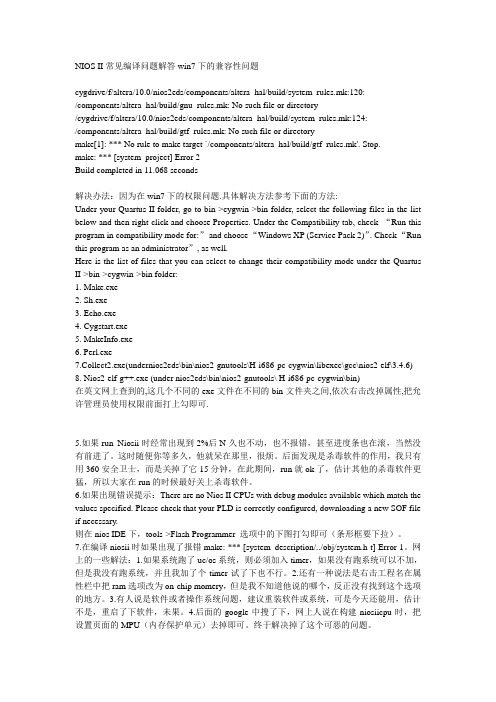
NIOS II常见编译问题解答win7下的兼容性问题cygdrive/f/altera/10.0/nios2eds/components/altera_hal/build/system_rules.mk:120:/components/altera_hal/build/gnu_rules.mk: No such file or directory/cygdrive/f/altera/10.0/nios2eds/components/altera_hal/build/system_rules.mk:124:/components/altera_hal/build/gtf_rules.mk: No such file or directorymake[1]: *** No rule to make target `/components/altera_hal/build/gtf_rules.mk'. Stop.make: *** [system_project] Error 2Build completed in 11.068 seconds解决办法:因为在win7下的权限问题.具体解决方法参考下面的方法:Under your Quartus II folder, go to bin->cygwin->bin folder, select the following files in the list below and then right-click and choose Properties. Under the Compatibility tab, check “Run this program in compatibility mode for:”and choose “Windows XP (Service Pack 2)”. Check “Run this program as an administrator”, as well.Here is the list of files that you can select to change their compatibility mode under the Quartus II->bin->cygwin->bin folder:1. Make.exe2. Sh.exe3. Echo.exe4. Cygstart.exe5. MakeInfo.exe6. Perl.exe7.Collect2.exe(undernios2eds\bin\nios2-gnutools\H-i686-pc-cygwin\libexec\gcc\nios2-elf\3.4.6)8. Nios2-elf-g++.exe (under nios2eds\bin\nios2-gnutools\ H-i686-pc-cygwin\bin)在英文网上查到的,这几个不同的exe文件在不同的bin文件夹之间,依次右击改掉属性,把允许管理员使用权限前面打上勾即可.5.如果run Niosii时经常出现到2%后N久也不动,也不报错,甚至进度条也在滚,当然没有前进了。
DDS(1)

Dynamic Mission Replanning
Image Processing & Tracking
DARPA PCES Capstone demo, 4/14/05, White Sands Missile Range
8
Tutorial on DDS
Douglas C. Schmidt
Case Study: QoS-enabled Publish/Subscribe Technologies for Tactical Information Management
Real-time Info to Cockpit Real-time Event Service Object Request Broker Tactical Network & RTOS
Problem: Net-centricity is afterthought 10 in platform-centric technologies
Goal is “better than best-effort,” subject to resource constraints… 12
Tutorial on DDS
Douglas C. Schmidt
Overview of the Data Distribution Service (DDS)
Applications
Interceptor Sys Cond Sys Cond Sys Cond Sys Cond
Applications
Interceptor
Middleware
Workload & Replicas
Local Resource Managers
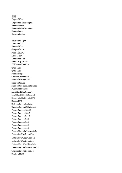
H264 baseline配置文件中文解释-JM12Encode
ANLMCS-TM-204 Nexus User's Guide
Table 2: Workstation-speci c Flags Flag
-n N -nodes S -Csave fds
N
Description Create N nodes on default processor Create nodes according to nodelist S Reserve N le descriptors
-sz N -on N -noc N -mbf N -mea N -pkt N
Description Number of nodes requested Single node to load program on Specify number of communication partners Specify bu er space for application Specify size of dedicated bu ers Specify message packet size
Description Start each context in debugger (if supported) Display for debugger windows (if supported) Pause on fatal and display id Pause on startup and display id Print commands without startup Disable catching of signals Enable catching of TRAP signal Enable catching of oating point exception
1 1 2
: : : : : : : : : : : : : : : : : : : : : : : : : : : : : : : : : : : : : : : : : : : : : : : : : : : : : : : : :
遮挡图像数据生成系统
光学 精密工程Optics and Precision Engineering第 29 卷 第 5 期2021年5月Vol. 29 No. 5May 2021文章编号 1004-924X(2021)05-1136-09遮挡图像数据生成系统梅若恒,马惠敏*(北京科技大学计算机与通信工程学院,北京100083)摘要:针对当前数据集在遮挡问题下对于目标检测算法系统评价的不足以及现实中部分数据难以获取的问题,本文提出一个遮挡图像数据生成系统来生成遮挡图像以及对应标注信息,并利用该系统构建遮挡图像数据集MOCOD(Morethan C-ommon Object Dataset ) °在系统构建方面,设计了场景及全局管理模块、控制模块和数据处理模块用于生成和处理数据从而构建遮挡图像数据集°在数据生成方面,使用模板ID 后处理图像生成不透明物体的像素级标注,使用光线 步进采样三维时序空间生成半透明物体的像素级标注,综合生成的标注数据计算出图像中目标物体的遮挡率并划分遮 挡等级°实验表明,吏用遮挡图像数据生成系统能够非常高效地标注实例分割级的标注数据,图像平均标注速度达到了0.07s °同时系统生成的标注数据提供10个等级的遮挡划分,相较于其他数据集有更为精确的遮挡等级划分和标注精度°系统引入的半透明物体遮挡标注也进一步增强了数据集对于遮挡问题评估的完备性°遮挡图像数据生成系统能够 高效地构建遮挡数据集,相较于其他现有数据集,本系统生成的数据集有更精确的标注信息,能够更好地评估目标检测算法在遮挡问题下的瓶颈和性能°关 键 词:遮挡;仿真;数据集;计算机视觉中图分类号:TP391 文献标识码:A doi :10. 37188/OPE. 20212905.1136Occlusion image data generation systemMEI Ruo -heng , MA Hui -min *(School of Computer & C o mmunication Engineering , University of S cience andTechnology Beijing , Beijing 100083, China )* Corresponding author , E -mail : :nhmpub@ustb . edu. cnAbstract : To address the inadequacy of current datasets for systematic evaluating target detection algo rithm under the occlusion problem and the difficulty in acquiring some data in reality , this paper proposesan occlusion image data generation system to generate images with occlusion and corresponding annota tions and to build the occlusion image dataset , namely more than common object dataset (MOCOD ). Interms of system architecture , a scene and global management module , a control module , and a data pro cessing module were designed to generate and process data to build an occlusion image dataset . In terms of data generation , for opaque objects , pixel -level annotation was generated via post -processing with a stencil buffer ; for translucent objects , the annotation was generated by sampling the 3D temporal space with raymarching. Finally , the occlusion level could be calculated based on the generated annotations. The experi ment result indicates that our system could efficiently annotate instance -level data , with an average annota tion speed of nearly 0. 07 s. The images provided by our dataset have ten occlusion levels. In the case of收稿日期:2020-08-25;修订日期:2020-10-27.基金项目:国家自然科学基金资助项目(No. 61773231)第5期梅若恒,等:遮挡图像数据生成系统1137MOCOD,the annotation is more accurate,occlusion level classification is more precise,and annotation speed is considerably faster,compared to those in the case of other datasets.Further,the annotation of translucent objects is introduced in MOCOD,which expands the occlusion types and can help evaluate the occlusion problem better.In this study,we focused on the occlusion problem,and herein,we propose an occlusion image data generation system to effectively build an occlusion image dataset,MOCOD;the accurate annotation in our dataset can help evaluate the bottleneck and performance of detection algorithms under the occlusion problem better.Key words:occlusion;simulation;dataset;computer vision1引言遮挡问题在计算机视觉领域一直是一个极具挑战的问题,当遮挡发生时,图像目标的特征会出现不同程度的缺失,造成目标检测算法精度的迅速下降。
HEVC-快速帧内编码
Fast intra mode decision algorithm for HEVC basedon dominant edge assent distributionYingbiao Yao &Xiaojuan Li &Yu LuReceived:24March 2014/Revised:22September 2014/Accepted:10November 2014#Springer Science+Business Media New York 2014Abstract As the latest video coding standard,high efficiency video coding (HEVC)is a successor to H.264/A VC.To improve the coding efficiency of intra coding,HEVC employs a flexible quad-tree coding block partitioning structure and 35intra prediction modes.The optimal prediction mode is selected through rough mode decision (RMD)and rate distortion optimisation (RDO)process.Due to the huge search space of all of the possible depth levels (CU sizes)and intra prediction modes,intra coding of HEVC is a very time-consuming and complicated process,which limits the application of HEVC.In order to reduce the intra coding complexity,we propose a fast mode decision algorithm for HEVC intra prediction which is based on dominant edge assent (DEA)and its distribution.The four DEAs in the directions of degree 0,45,90and 135are computed first;then,the dominant edge is decided according to the minimum DEA.Next,a subset of prediction modes in accordance with the dominant edge is chosen for the RMD process.The rule is as follows:When the standard deviation of DEA is distinctly small,we skip the RMD process and take the direct current (DC)mode and planar modes as the candidate modes for the RDO process;when the minimum DEA is distinctly small,we select seven modes as the candidate modes for the RMD process;otherwise,we select 11modes for the RMD stly,the prediction unit (PU)size-based number of RDO candidate modes (3for PU size 4×4and 8×8and 1for the other PU sizes)is modified according to experimental pared with HM 9.1,Shen ’s proposal and da Silva ’s proposal,which are two state-of-the-art fast intra mode decision algorithms,the experimental results reveal that the proposed algorithm can save 36.26,13.85and 20.81%coding time on average with a negligible loss of coding efficiency,respectively.Keywords HEVC .Mode decision .Intra prediction .Dominant edge assent distribution DOI10.1007/s11042-014-2382-7This work was supported in part by the National Natural Science Foundation of China under Grant No.61100044and Zhejiang Provincial Natural Science Foundation of China under Grant No.LY12F01007.Y .Yao (*):X.Li :Y .LuCollege of Communication Engineering,Hangzhou Dianzi University,Hangzhou 310018,People ’s Republic of Chinae-mail:yaoyb@X.Lie-mail:354577289@Y .Lue-mail:y_lu@1IntroductionHigh efficiency video coding(HEVC)is the latest video coding standard developed by the Joint Collaborative Team on Video Coding(JVC-TC)[20].HEVC is aimed to substantially improve coding efficiency compared with its predecessor H.264/A VC;it employs many state-of-the-art techniques and algorithms,and these tools greatly contribute to meeting the goal of reducing the bitrates by half while keeping comparable video quality compared to H.264/A VC High Profile[14].The official version of the HEVC standard was issued in February2013and still uses block-based hybrid coding architecture.For intra prediction,it employs a flexible quad-tree coding block partitioning structure and a multi-angle intra prediction method[18].The partitioning structure of the quad-tree coding block introduces three block concepts:coding unit(CU),prediction unit(PU)and transform unit(TU),which enables the efficient use of large and multiple sizes of coding,prediction and transform blocks.CU is the elementary unit of region splitting used for inter/intra prediction;its size can range from8×8to64×64in the test model of HEVC(HM)[13].The CU concept allows for recursive splitting into four equal blocks,as shown in Fig.1.PU is the elementary unit for prediction and is defined after the last Fig.1Illustration of recursive CU structure in HEVCdepth level of CU splitting.For intra prediction,two PU sizes are supported at each depth level:2N×2N and N×N.The types of PU are64×64,32×32,16×16,8×8and4×4.TU is the unit for transform and quantisation.The multi-angle intra prediction method offers35 modes,including33direction modes,a direct current(DC)mode and a planar mode,as shown in Fig.2.The flexible block structure better adapts to the image coding,and a large number of prediction modes greatly improve the prediction precision.Just like the predecessor H.264/A VC,the intra mode decision process in HEVC is to utilise the rate distortion optimisation(RDO)process to find the mode with the least rate distortion (RD)cost in all of the possible depth levels(CU sizes)and intra prediction modes.The RD cost function(J RDO)used in HM is evaluated as follows:J RDO¼SSEþλÂBð1Þwhere SSE is the sum of square error of current CU and the matching blocks,λis the Lagrange multiplier and B specifies the bit cost to be considered for mode decision,which depends on each decision case.The process of RDO calculation is very complex.Moreover,the technologies of flexible block structure and many prediction modes add to the number of RDO calculations;therefore it is a very time-consuming and complicated process for the HEVC encoder to utilise RDO by traversing all combinations of CU,PU and TU sizes and35modes for each block.The complexity greatly limits the application of HEVC;thus,how to reduce the HEVC intra Fig.2Thirty-five intra prediction modes in HEVCcoding complexity on the premise of guaranteeing coding performance has been become one of the research hotspots in the practical application of HEVC.In this paper,we proposed a fast HEVC intra mode decision algorithm to reduce the complexity of intra encoding.Based on dominant edge assent and its distribution,our algorithm can flexibly choose a different number of prediction modes as candidate modes for the RMD and RDO processes.The major contributions of this paper are as follows:1)We improve the mode classification method in[6]by taking advantage of the effective edgedirection detection method,which is based on dominant edge assent(DEA)in[19].Instead of categorising modes into five types and determining the type by utilising five different filters in[6],our DEA-based method classifies35intra prediction modes into four types at the followingdegrees:0,45,90and135.Each type has11intra prediction modes for the RMD process.2)We further reduce the number of prediction modes for the RMD process by the distribu-tion of DEA,including its standard deviation and the difference between the second lowest value and the minimum value.According to the difference and standard deviation of DEA,seven or eleven prediction modes are selected as candidate modes for the RMD process;in a particular case,we skip the RMD process.3)We modify the PU size-based number of modes selected from the RMD process(3for PUsize4×4and8×8and1for the other PU sizes);thus,fewer modes are applied in the RDO calculation.4)We integrate the proposed algorithm into the test model HM9.1and conduct an extensiveperformance evaluation.We compare the△Bitrate,△PSNR,△T,BD-Rate and BD-PSNR of the proposed algorithm with those of HM9.1,Shen’s proposal in[17]and da Silva’s proposal in[6],which are two state-of-the-art fast intra mode decision algorithms.The results show that the proposed algorithm can save36.26,13.85and20.81%coding time on average with a negligible loss of coding efficiency over HM9.1,Shen’s proposal and da Silva’s proposal,respectively.The remainder of this paper is organised as follows.Section2reviews related works. Section3presents a detailed description of the proposed fast intra mode decision algorithm. Section4shows the experimental results.Finally,Section5concludes the paper.2Related worksRecently,much attention has been paid to fast HEVC intra coding algorithms,which can be classified into three types:simplifying RD cost function in[9,16],fast block partitioning in[5, 10–12,17,21]and fast mode decision in[3,4,6–8,15,22].In this section,we briefly discuss the intra coding algorithms,especially fast block partitioning algorithms and fast mode decision algorithms.In[16],a hadamard cost-based RMD process is introduced to choose N best candidate intra modes.Only N candidate modes are tested in the RDO process,instead of testing all of the modes.Since RMD is much less time-consuming,it can substantially save encoding time and is adopted in the first test model of HM1.0.Zhao et al.[22]further reduce the candidate modes,which are selected from the RMD process to cut down RDO calculation;meanwhile, they make full use of the direction information of the neighbouring blocks and add the most probable mode(MPM)of neighbouring blocks to the candidate mode set for the RDO process. Zhao’s proposal is partly adopted in HM2.0.In subsequent versions of test model HM,the intra encoding framework changes little.Works in[5,10–12,17,21]use fast block partitioning algorithms by employing coding block structure to speed up the intra coding process.Shen et al.[17]skip the coding process of seldom-used depth level when partitioning a coding block;they also fully utilise the RD cost and prediction mode correlations among different depth levels or spatially nearby CUs to skip some prediction modes that are rarely used in the parent CUs of the upper depth levels or spatially nearby CUs.According to the spatial and temporal correlation between adjacent CUs, Yan et al.[21]predict the depths of coding block by using the optimal depths of adjacent CUs. In[11],Kim et al.analyse the correlation between RD costs and block size.During the process of block partitioning,they terminate the sub-block dividing by comparing RD cost with the threshold value given by experiments.Furthermore,the authors in[5]also analyse the correlation between block size and hadamard cost in the RMD process cost.They skip the unnecessary coding process of large-size coding block and terminate the sub-block partitioning by using the hadamard cost and RD cost.According to the principle that prediction residual can reflect prediction accuracy,Ma et al.[12]terminate their block division by comparing prediction residual with the threshold value given by their experiments.Khan et al.[10] consider the correlation between video texture feature and the variance of pixel values to simplify the coding block segmentation process.Fast mode decision algorithms can also be found in the literature[3,4,6–8,15].As mentioned in[15],since pixels along the direction of the local edge are normally of similar values,a good prediction could be achieved if we predicted the pixels using the neighbouring pixels that are in the same direction as the edge.Jiang et al.[8]calculate the gradient directions of current PUs’pixels and use the gradient-mode histogram to choose a reduced set of candidate prediction directions for RMD calculation.Chen et al.[4]use a similar method to Jiang’s in the RDO process and reduce the number of candidate prediction modes for RDO as well.Chen et al.[3]introduce the conception of kernel density estimation into the histogram calculation,which improves the robust-ness of the edge direction statistics.As the calculation of each pixel’s gradient information requires much time,fast intra mode decision algorithms in[6,7,19]extract the edge information of each encoding block rather than each pixel.For H.264intra prediction,the authors in[19]effectively estimate the edge direction inside the block by employing dominant edge assent to narrow down the prediction modes to reduce the RDO calculation.Da Silva et al.[6] apply five different filters to detect the dominant edge;then,they choose a subset of the prediction modes in accordance with the detected dominant edge for the RMD calculation.Fang et al.[7]exploit direction energy distribution to select a subset of the prediction modes for the RMD process.Although these algorithms can be used to reduce the computational complexity of HEVC,considering the new features of the current block’s dominant edge statistics can further reduce the complexity.3Proposed fast intra mode decision algorithmFigure3describes the intra mode decision algorithm in HM9.1.There are three steps: the RMD process,the process of adding MPM into the candidate set and the RDO process.To avoid checking all of the intra modes in the RMD process and further reducing the candidate modes of the RDO calculation,we propose a fast mode decision algo-rithm that significantly reduces the encoder complexity.The detailed algorithm is described next.3.1DEA-based mode decision3.1.1Prediction mode classificationIn order to reduce the coding complexity by selecting reduced modes for the RMD process,we first consider classifying the intra prediction modes.As described in[6],da Silva et al.give five subsets of prediction modes associated with five types of edge(four directional,0,45,90, 135°,and one non-directional edge).The dominant edge is detected by using five different filters;it can save a great deal of time by choosing a subset of prediction modes for RMD calculation rather than all prediction modes.Instead of categorising the edges into five types and detecting the dominant edge by using five different filters in[6],our method offers four directional edge types,except the non-directional edge type,which can be detected by analysing the dominant DEA of the current block.Figure4shows the candidates of the directional modes in accordance with the different dominant edge directions.The candidate directional modes are composed of the mode corresponding to the dominant edge direction and the eight adjacent angular modes that are most often selected as the best mode.Modes of14,22and30belong to two adjacent types of edge.In order to retain prediction performance in a smoother block,the DC mode and planar mode are always chosen for the RMD process.Table1shows the four kinds of subsets of candidate prediction modes in accordance with the different dominant edge directions.Each subset contains only11modes rather than35modes for RMD calculation.3.1.2Dominant edge assentIn order to determine the prediction mode type,we detect the dominant edge by employing DEA in[19].As described in[19],an N×N-size PU is equally divided into four N/2×N/2-size parts and an N/2×N/2-size central part,shown in Fig.5.The average pixel values of each part are computed as(2)-(6).p a¼Xi¼N2−1i¼0Xj¼N2−1j¼0p i j.NÂN4ð2Þp b¼Xi¼N−1i¼N2Xj¼N2−1j¼0p i j.NÂN4ð3ÞFig.3Intra mode decision procedure for a depth level in HM9.1p c ¼X i ¼N 2−1i ¼0X j ¼N −1j ¼N 2p i j .N ÂN 4ð4Þp d ¼X i ¼N −1i ¼N 2X j ¼N −1j ¼N 2p i j .N ÂN 4ð5Þp e ¼X i ¼3N 4−1i ¼N 4X j ¼3N 4−1j ¼N 4p i j .N ÂN 4ð6Þwhere p ij indicates the pixel value at the position (i ,j )of the N×N-size PU.Fig.4Modes in accordance with four dominant edgesTable 1Subsets of prediction modes in accordance with the detected dominant edge directionDominant edge directionSubset of modes chosen for RMD calculation 0°6,7,8,9,10,11,12,13,14,0,145°2,3,4,5,30,31,32,33,34,0,190°22,23,24,25,26,27,28,29,30,0,1135°14,15,16,17,18,19,20,21,22,0,1After getting p a ,p b ,p c ,p d and p e ,the four dominant direction assents DEA 1,DEA 2,DEA 3and DEA 4at degree 0,45,90and 135are given by the following:DEA 1¼p b −p a j j þp d −p c j jð7ÞDEA 2¼p c −p e j j þp e −p b j jð8ÞDEA 3¼p c −p a j j þp d −p b j jð9ÞDEA 4¼p d −p e j j þp e −p a j j ð10ÞTheoretically,the direction in accordance with the minimum dominant edge assent (DEA min )is the dominant edge.DEA min is obtained by the following:DEA min ¼Min DEA 1;DEA 2;DEA 3;DEA 4f g ð11ÞWe decide the right mode type according to the dominant edge direction detected.Thus,we can choose the right subset of prediction modes to do the RMD process from Table 1.Then,fewer modes selected in the RMD process as well as MPM will be applied in the RDO process.Theoretically,a great deal of coding time can be saved.3.1.3Mode decision method verificationIn order to verify the accuracy of our method,we employ five sequences in different resolutions with the quantisation parameters 22,27,32and 37.Table 2shows the percentage of the optimal prediction mode that is included in the candidate set for the RDO process selected by our method.The average percentage is up to 92.57%,which verifies the accuracy of our method.The theoretical and experimental results show that our modified mode decision method can save coding time and guarantee the quality of the pictures.NN p ap b p c p dp eFig.5N×N-size PU partition into five N/2×N/2-size sub-blocks3.2DEA distribution-based mode decisionAs described in Section 3.1,the DEA-based mode decision algorithm selects 11modes from all of the prediction modes for the RMD calculation,which saves time compared to applying all of the modes to the RMD process.Considering the obvious properties of orientation and smoothness,the subset modes can be further reduced.Since the calculated DEA indicates the information about edge direction,we can apply its distribution to check the properties of obvious orientation and smoothness.3.2.1Obvious directional coding blockOn the one hand,we find that if the PU is obviously directional,the minimum DEA (DEA min )in accordance with the edge direction is distinct and very small;thus,the obvious orientation can be decided by the difference between the second smallest value of DEA (DEA secmin )and DEA min .DEA min can be obtained by (11).DEA secmin is the smallest value among the DEA s except for DEA min ,defined by function SecMin.DEA secmin can be obtained by (12):DEA secmin ¼SecMin DEA 1;DEA 2;DEA 3;DEA 4f g ð12ÞWe define a threshold (Th min )to decide whether the PU is obviously directional.We assume that the PU is obviously directional if the DEA meets (13):DEA secmin −DEA min >Th min ð13ÞWhen the current PU is very directional rather than smooth,the DC mode and planar mode should be rejected from the prediction modes subset.Considering the detected strong direc-tional property,the subset modes in Table 1should be further reduced.We reduce the adjacent modes,whose direction is in accordance with the dominant edge direction.Further,we employ the subsets shown in Table 3when we detect that the PU is very directional.The candidate is composed of the mode corresponding to the dominant direction and six adjacent angular modes.Table 2Percentage of the optimal prediction mode being included in the selected candidate set for RDO SequencesResolution (pixels)Percentage (%)Traffic2560×160088.14Kimono11920×108090.25Flowervase832×48095.67Mobisode2416×24096.95Four people1280×72091.85Average 92.57Table 3Subsets of prediction modes when the PU is obviously directionalDominant edge directionSubset of modes chosen for RMD calculation 0°7,8,9,10,11,12,1345°2,3,4,31,32,33,3490°23,24,25,26,27,28,29135°15,16,17,18,19,20,21In order to obtain the value of Th min ,we employ sequences in Table 2with the quantisation parameters 22,27,32and 37to check coding efficiency at different threshold values.An example of RD curves of Kimono1(1920×1080)at different threshold values is shown in Fig.6.We test different Th min values of 30,40and 50by coding 10frames of the sequence Kimono1.The RD curves at different threshold Th min are close to the curve of HM 9.1.The coding efficiency measured by BD-Rate (%)and BD-PSNR (dB)is shown in Table 4.According to Table 4and Fig.6,we can deduce that the threshold Th min should be around40.By analysing the extensive experimental results,we set the threshold Th min as 43.Table 5shows the percentage of the optimal prediction mode that is included in the candidate set for the RDO process obtained by the above methods.From Table 5,we find that the percentages are similar to that of Table 2,which verifies the accuracy of our method.3.2.2Obvious smooth coding blockOn the other hand,when the PU is extremely smooth,the DC mode or the planar mode will be most likely to be the optimal prediction mode.In this case,we skip the RMD process,and only the DC mode,planar mode and MPM are applied in the RDO calculation.If the DEAs of the four dominant edge directions are almost equal to one other,we can deduce that the PU is not directional,but that it is very smooth.We then employ the standard deviation of the four DEAs (DEA dev )to decide whether the PU is obviously smooth.DEA dev is given by (14)and (15).DEA dev ¼ffiffiffiffiffiffiffiffiX i ¼14s DEA i −u ðÞ2.2ð14Þu ¼Xi ¼14DEA i .4ð15ÞFig.6RD curves of Kimono1at different threshold values of Th minTable4Coding efficiency at different Th min compared with HM9.1Th min BD-Rate(%)BD-PSNR(dB)3079.53−0.0282 4076.04−0.0268 5078.47−0.0277We assume that the PU is extremely smooth when DEA dev meets(16):DEA dev<Th devð16Þwhere Th dev is a threshold that optimises the trade-off between coding time and coding efficiency.To derive the value of Th dev,we employ the sequence of Vidyo1(1280×720),the texture of which is plain,with the quantisation parameters22,27,32and37.The statistics of DEA dev are created when the optimal prediction mode is DC mode or planar mode.The mean of DEA dev is 2.3and the median of DEA dev is0.98.We test coding efficiency and coding time when Th dev is 2,1.5,1.0,0.95and0.9.The results show that the smaller Th dev is,the better coding the efficiency is;whereas the larger Th dev is,the more coding time can be saved.Table6shows the percentage of the optimal prediction mode that is included in the candidate set for the RDO process when we set the threshold Th dev as0.95.The percentages do not decrease very much compared with the above percentages.Considering the trade-off between coding time and coding efficiency,it is suitable to set the threshold Th dev as0.95.3.3PU size-based number of RDO candidate modesThe above method indicates that less intra prediction modes,instead of all intra prediction modes,are selected for the RMD calculation.After the RMD process,as Fig.3indicates,N prediction modes will be selected and the N modes as well as MPM will be applied in the RDO process to determine the optimal prediction mode.In HM9.1,N is3or8,according to the PU size.Through the experimental analysis,we find that keeping the original value of N cannot improve the coding performance greatly,but instead wastes time checking more modes in the RDO process.To further reduce the complexity of the encoder,different settings of N are checked.For the PU size of4×4and8×8,the values of6,4,3and2are checked.For the PU Table5Percentage of the optimal prediction mode being included in the selected candidate set for the RDO Sequences Resolution(pixels)Percentage(%)Traffic2560×160088.07 Kimono11920×108090.24 Flowervase832×48095.64 Mobisode2416×24096.92Four people1280×72091.83 Average92.54Table6Percentage of the optimal prediction mode included in the selected candidate set for the RDO Sequences Resolution(pixels)Percentage(%)Traffic2560×160087.25 Kimono11920×108089.48 Flowervase832×48094.93 Mobisode2416×24095.89Four people1280×72091.00 Average91.71sizes of16×16,32×32and64×64,the values of3,2and1are checked.Finally,considering the trade-off between the performance and complexity,we set N as3for PU size4×4and8×8 and1for other PU sizes,as shown in Table7.The experimental results show that a smaller N can save a great deal of coding time with the similar coding performance of the above algorithms.3.4Overall algorithmBased on the above analysis,we propose a fast intra mode decision algorithm for HEVC based on dominant edge assent distribution,as shown in Fig.7.Step1Compute DEA and DEA min respectively based on(7)–(10)and(11)for a PU block.The direction indicated by DEA min is the dominant edge direction.Step2Compute DEA dev based on(14).When DEA dev meets(16),skip the RMD process and take the DC mode and the planar mode as the candidate modes selected from RMD.Then go directly to Step6.Step3Compute DEA secmin based on(12).If the difference of DEA secmin and DEA min meets(13),select seven modes,referring to Table3as the candidates for the RMD process,and go to Step5.Step4Select11modes,referring to Table1as the candidates for RMD process,and go to Step5.Step5Do the RMD process.Check seven or11intra prediction modes based on SATD, which are chosen by Step3or Step4,and select N candidates for the RDO calculation.N is3for PU sizes4×4and8×8and1for other PU sizes;then,go to Step6.Step6Check whether MPM is included in the candidates of the RDO process.If MPM is not included in the candidate set,N+1modes,comprised of N best modes of RMD and a MPM,will be employed in the RDO process.Otherwise,only N best modes will be employed in the RDO process.Step7Do the RDO calculation to find out the optimal prediction mode from the candidates.Table7Number of modes selected from the RMD process for different PU sizes in our algorithmPU size N4×4or8×83 Other14Experiment results4.1Efficiency analysisIn order to analyse the efficiency of our proposed algorithm,we give the statistic for average mode number of RMD and RDO candidates for five sequences in different resolutions with the quantisation parameters22,27,32and37.Table8shows the average number of RMD candidates of HM9.1and our proposed algorithm.Table9 shows the average number of RDO candidates of HM9.1and our proposed algorithm. We find that our proposed algorithm greatly reduces the modes of RMD calculation and RDO calculation.Because of the simpler calculation of DEA and its distribution compared with RMD and RDO,the proposed algorithm can save much encoding time and reduce the calculation complexity significantly.Fig.7Mode decision flow chart(The procedures in grey blocks represent our proposed algorithm.)4.2Performance analysisTo verify the performance of the proposed fast intra mode decision,we implemented it in the test model HM 9.1of HEVC.Experiments are carried out for all I-frames sequences.The recommended video sequences specified by [2]in four resolutions (416×240,832×480,1920×1080and 2560×1600formats)and quantisation parameter values of 22,27,32and 37are implemented.Table 10shows the comparison results between the proposed algorithm and HM 9.1in terms of coding efficiency and computational complexity.The coding efficiency is measured by BD -Rate (%)and BD -PSNR (dB)[1].Furthermore,the percentage difference in bitrate (△Bitrate ),the luminance PSNR difference (△PSNR )and the percentage difference in encoding time (△T )are also used to compare our algorithm with HM 9.1.Positive and negative values represent increments and decrements,respectively.The criteria are calculated as (17)–(19).ΔBitrate ¼Bitrate proposed −Bitrate HM 9:1Bitrate HM 9:1Â100%ð17ÞΔPSNR ¼PSNR proposed −PSNR HM 9:1ð18ÞΔT ¼T proposed −T HM 9:1HM 9:1Â100%ð19ÞExperimental results reveal that the proposed algorithm can save an encoding time of about 36%on average,whereas the average increase of bitrate is only 0.57%and the average degradation of PSNR is 0.07dB over all test sequences.However,the simulation with theTable 9Average number of RDO candidates Sequences HM 9.1Proposed algorithm Traffic 7.95 3.17Kimono17.88 2.92Flowervase 7.79 2.69Mobisode27.75 2.48Four people 7.92 3.10Average7.862.87Table 8Average number of RMD candidates Sequences HM 9.1Proposed method Traffic 357.48Kimono1357.60Flowervase 35 3.19Mobisode235 1.98Four people 35 6.00Average355.24。
ANSYS软件错误锦集
ANSYS软件错误锦集1 在Ansys中出现“Shape testing revealed that 450 of the 1500 new or modified elements violate shape warning limits.”,是什么原因造成的呢?单元网格质量不够好,尽量用规则化网格,或者再较为细密一点。
2 在Ansys中,用Area Fillet对两空间曲面进行倒角时出现以下错误:Area 6 offset could not fully converge to offset distance 10. Maximum error between the two surfaces is 1% of offset distance.请问这是什么错误?怎么解决?其中一个是圆柱接管表面,一个是碟形封头表面。
ansys的布尔操作能力比较弱。
如果一定要在ansys里面做的话,那么你试试看先对线进行倒角,然后由倒角后的线形成倒角的面。
建议最好用UG、PRO/E这类软件生成实体模型然后导入到ansys。
3 在Ansys中,出现错误“There are 21 small equation solver pivot terms。
”,是否是在建立接触contact时出现的错误?不是建立接触对的错误,一般是单元形状质量太差(例如有接近零度的锐角或者接近180度的钝角)造成small equation solver pivot terms4 在Ansys中,出现警告“SOLID45 wedges are recommended only in regions of relatively low stress gradients.”,是什么意思?"这只是一个警告,它告诉你:推荐SOLID45单元只用在应力梯度较低的区域。
它只是告诉你注意这个问题,如果应力梯度较高,则可能计算结果不可信。
"5 ansys向adams导的过程中,出现如下问题“There is not enough memory for the Sparse Matrix Solver to proceed.Please shut down other applications that may be running or increase the virtual memory on your system and return ANSYS.Memory currently allocated for the Sparse Matrix Solver=50MB.Memory currently required for the Sparse Matrix Solver to continue=25MB”,是什么原因造成的?不清楚你ansys导入adams过程中怎么还需要使用Sparse Matrix Solver(稀疏矩阵求解器)。
- 1、下载文档前请自行甄别文档内容的完整性,平台不提供额外的编辑、内容补充、找答案等附加服务。
- 2、"仅部分预览"的文档,不可在线预览部分如存在完整性等问题,可反馈申请退款(可完整预览的文档不适用该条件!)。
- 3、如文档侵犯您的权益,请联系客服反馈,我们会尽快为您处理(人工客服工作时间:9:00-18:30)。
NoC System for MPEG-4 SP using heterogeneous tiles
Antoni Portero, Guillermo Talavera, Marius Montón, Borja Martínez, Jordi Carabina Dep. MiSE ETSE 08193 Bellaterra Spain {name.surname}@uab.es
Abstract.- In this paper we present a high level methodology to get optimal work points for a MPEG-4 Single Profile implementation. The flow goes from a C++ description of a MPEG-4 encoder to a SystemC implementation. Afterwards, code is migrated to an architecture processor research framework (trimaran) and a real implementation on an Altera FPGA and on a DSP. These different implementations are possible tiles in a mesh NoC that is modelled in TLM level and afterward synthesized with a high level synthesis tool.
1. INTRODUCTION Currently, one of the most challenging issues in the telecom market segment is to manage the growing complexity of embedded multimedia systems and to reduce their design productivity gap. These elements stimulate a continuous development of industrial methodologies and flows design exploiting reuse, extended verification, and high level-synthesis. SystemC [1] is a system-level design language that allows modelling and verification of complex HW/SW components. Starting from some tool-dependent HW coding styles (e.g. Forte Design Systems Cynthesizer), it is possible to reach the silicon platforms out of an industrial design flow. Furthermore, the emergence of high capacity reconfigurable devices is starting a revolution in its use for general-purpose computing applications. Many coarse-grain reconfigurable architectures appeared as reconfigurable coprocessors, structures ASICs, etc. considerably relieving the burden from the main processor in many multimedia applications due to their very high degree of parallelism. In addition, they generally have wider flexibility than an application specific circuit. TLM (Transaction Level Modelling) SystemC description permits a rapid system development. Parts of the systems are locally synchronized by a clock but globally there is a handshaking or a shared-bus communication. When we try to synthesize we do not know exactly the number of resources and clock timing of each tile. Hence, GALS philosophy (Globally Asynchronous Locally Synchronous) make independent computation and communication. Any tile of the system can be connected to another if they have the same protocol. The communication to connect a tile and the NoC is based on a burst transfer to an AMBA bus [2]. Following SoC evolution driven by the increase in integration density, NoCs (Networks on a Chip) [2] are being used as a communication infrastructure between tiles containing IPs (Intellectual Property blocks). OCP-IP organization is leading a community trying to standardize the communication protocols and promote the development of tools to automate the NoC strategy for multiprocessor System-on-Chip. This paper shows an efficient use of NoCs to interconnect several replicated tiles of a MPEG-4 Single Profile implementation with different computation requirements. The NoC employs packet switching, a communication mechanism in which packets are individually routed between cores, with no previously established path [4]. The wormhole packet switching mode is used to avoid the need for large buffer spaces. The routing algorithm defines the path taken by a packet between the source and the destination. The deterministic algorithm is employed. The system will have a manager that will decide the tile assignment according to performance requirements, basically execution time versus power consumption. Paper is divided in seven parts; first section is a description of our IPs MPEG-4SP and NoC, second part explains Systemc development. Third part, describes the tiles that are connected to the network. Part fourth briefly the energy model that we have used. Fifth part gives details about the different possible target platforms for the Network tile. Part six presents some results. Finally, part seven explains conclusions and future work.
1. MPEG-4 SP TILE DESCRIPTION The starting point of the flow was a C++ specification of the MPEG4 standard. From this specification we built a MPEG-4 single profile code without dynamic memory allocation and without pointers needed to offer a posterior SystemC synthesis [5].
DCIS 2006