Predicting BER with IBIS-AMI_eperiences correlating SerDes simulations and measurement
泰克示波器增加基于IBIS-AMI模型和S参数的建模功能

t o r i z e d P o we r Ar c h i t e c t u r e , F P A) 方案, 来 分 隔 元 件 之 间 的 调 控 和 电 压 转换 。两 个 高 度 集 成 的 电 源 处 理 模 块 内 的 分 别 调控 和 转换 , 实 现 了整 个 价 值 指 标 范 围 的 卓 越 性 能 ,
替 准 确性 较 低 的参 考均 衡 模 型 。对 I B I S—AMI的支 持 是
S e r i a l Da t a L i n k An a l y s i s Vi s u a l i z e r ( S DLA Vi s u a l i z e r ) 软
5 0 0 M Hz 、 5 Gs / s实 时采 样 率 的 四 通 道 手 持 式 示 波 器 , 采 用密封 、 坚 固 的设 计 , 并 且提 供最 高 C ATI V6 0 0 V 安 全 等
人员观察波形细节 。
扩 展 其 数 字 增 强 型 电 源 模 拟 控 制 器 产 品 线 。随 着 全 新 器 件 MC P 1 9 1 l 4和 MC P1 9 1 1 5的 推 出 , Mi c r o c h i p智 能 DC / DC电 源 转 换 解 决 方 案 更 加 多 元 化 , 其 控 制 器 系 列 现 已 发 展 到 可支 持 反 激 式 、 升 压和 S E P I C 等 多 种 拓 扑 结 构 。新 器 件 引人 了一 个 升 压 P W M 控 制 器 和 下 桥 臂 MOS FE T 驱 动 器 的架 构 , 以及 一 个 中压 L DO 和全 功 能单 片 机 , 所 有 这
..
『  ̄ D u s f
圈
( E S D保护) 以及 电 源 对 地 / 电池的短 路保护 , 同 时 该 芯 片
alibi 原理

Alibi原理解析简介Alibi是一个用于解释和可信度评估机器学习模型的Python库。
它提供了一系列的技术和工具,可以帮助我们理解模型的预测结果,并评估模型的可靠性。
Alibi 主要关注两个方面:解释性和可信度评估。
解释性解释性是指我们能够理解模型为什么会做出某个特定的预测。
在实际应用中,解释性对于决策制定者、监管机构以及最终用户来说都非常重要。
Alibi提供了多种方法来实现模型的解释性,包括特征重要性分析、局部影响分析和对抗样本生成等。
特征重要性分析特征重要性分析是指确定哪些特征对于模型预测结果的贡献最大。
Alibi提供了多种方法来计算特征重要性,包括经典的Permutation Importance和SHAP (SHapley Additive exPlanations)等。
Permutation Importance通过随机改变一个特征的值并观察预测结果的变化来衡量该特征对于预测结果的影响。
如果改变某个特征的值几乎不会改变预测结果,那么该特征的重要性就较低。
SHAP是一种基于博弈论的方法,它将每个特征的贡献分配给不同的特征子集。
SHAP值表示了每个特征对于预测结果的影响程度,可以帮助我们理解模型是如何利用各个特征来做出决策的。
局部影响分析局部影响分析是指确定某个样本中每个特征对于模型预测结果的贡献。
Alibi提供了多种方法来计算局部影响,包括LIME(Local Interpretable Model-agnostic Explanations)和Anchor等。
LIME通过在原始样本附近生成一组新样本,并使用一个简单可解释的模型来近似原始模型。
通过比较这些新样本与原始样本之间的差异,我们可以得到每个特征对于预测结果的贡献。
Anchor是一种更加直观和可理解的局部影响分析方法。
它基于规则(如IF-THEN 规则)来解释模型预测结果,可以帮助我们理解为什么模型会做出某个决策。
对抗样本生成对抗样本生成是指通过小幅度修改输入数据,使得模型产生错误的预测结果。
riskclustr包的说明文档说明书

Package‘riskclustr’October14,2022Type PackageTitle Functions to Study Etiologic HeterogeneityVersion0.4.0Description A collection of functions related to the study of etiologic heterogeneity both across dis-ease subtypes and across individual disease markers.The included functions allow one to quan-tify the extent of etiologic heterogeneity in the context of a case-control study,and provide p-values to test for etiologic heterogeneity across individual risk factors.Begg CB,Za-bor EC,Bernstein JL,Bernstein L,Press MF,Seshan VE(2013)<doi:10.1002/sim.5902>. Depends R(>=4.0)License GPL-2URL /riskclustr/,https:///zabore/riskclustrBugReports https:///zabore/riskclustr/issuesEncoding UTF-8Imports mlogit,stringr,MatrixLanguage en-USLazyData trueRoxygenNote7.1.0VignetteBuilder knitrSuggests testthat,covr,rmarkdown,dplyr,knitr,usethis,spellingNeedsCompilation noAuthor Emily C.Zabor[aut,cre]Maintainer Emily C.Zabor<***************>Repository CRANDate/Publication2022-03-2301:00:02UTC12d R topics documented:d (2)dstar (3)eh_test_marker (4)eh_test_subtype (5)optimal_kmeans_d (7)posthoc_factor_test (8)subtype_data (9)Index11d Estimate the incremental explained risk variation in a case-controlstudyDescriptiond estimates the incremental explained risk variation across a set of pre-specified disease subtypesin a case-control study.This function takes the name of the disease subtype variable,the number of disease subtypes,a list of risk factors,and a wide dataset,and does the needed transformation on the dataset to get the correct format.Then the polytomous logistic regression model isfit using mlogit,and D is calculated based on the resulting risk predictions.Usaged(label,M,factors,data)Argumentslabel the name of the subtype variable in the data.This should be a numeric variable with values0through M,where0indicates control subjects.Must be suppliedin quotes,bel="subtype".quotes.M is the number of subtypes.For M>=2.factors a list of the names of the binary or continuous risk factors.For binary risk factors the lowest level will be used as the reference level.e.g.factors=list("age","sex","race").data the name of the dataframe that contains the relevant variables.ReferencesBegg,C.B.,Zabor,E.C.,Bernstein,J.L.,Bernstein,L.,Press,M.F.,&Seshan,V.E.(2013).A conceptual and methodological framework for investigating etiologic heterogeneity.Stat Med,32(29),5039-5052.doi:10.1002/sim.5902dstar3 Examplesd(label="subtype",M=4,factors=list("x1","x2","x3"),data=subtype_data)dstar Estimate the incremental explained risk variation in a case-only studyDescriptiondstar estimates the incremental explained risk variation across a set of pre-specified disease sub-types in a case-only study.The highest frequency level of label is used as the reference level,for stability.This function takes the name of the disease subtype variable,the number of disease sub-types,a list of risk factors,and a wide case-only dataset,and does the needed transformation on the dataset to get the correct format.Then the polytomous logistic regression model isfit using mlogit, and D*is calculated based on the resulting risk predictions.Usagedstar(label,M,factors,data)Argumentslabel the name of the subtype variable in the data.This should be a numeric variable with values0through M,where0indicates control subjects.Must be suppliedin quotes,bel="subtype".quotes.M is the number of subtypes.For M>=2.factors a list of the names of the binary or continuous risk factors.For binary risk factors the lowest level will be used as the reference level.e.g.factors=list("age","sex","race").data the name of the case-only dataframe that contains the relevant variables.ReferencesBegg,C.B.,Seshan,V.E.,Zabor,E.C.,Furberg,H.,Arora,A.,Shen,R.,...Hsieh,J.J.(2014).Genomic investigation of etiologic heterogeneity:methodologic challenges.BMC Med Res Methodol,14,138.4eh_test_marker Examples#Exclude controls from data as this is a case-only calculationdstar(label="subtype",M=4,factors=list("x1","x2","x3"),data=subtype_data[subtype_data$subtype>0,])eh_test_marker Test for etiologic heterogeneity of risk factors according to individualdisease markers in a case-control studyDescriptioneh_test_marker takes a list of individual disease markers,a list of risk factors,a variable name denoting case versus control status,and a dataframe,and returns results related to the question of whether each risk factor differs across levels of the disease subtypes and the question of whether each risk factor differs across levels of each individual disease marker of which the disease subtypes are comprised.Input is a dataframe that contains the individual disease markers,the risk factors of interest,and an indicator of case or control status.The disease markers must be binary and must have levels0or1for cases.The disease markers should be left missing for control subjects.For categorical disease markers,a reference level should be selected and then indicator variables for each remaining level of the disease marker should be created.Risk factors can be either binary or continuous.For categorical risk factors,a reference level should be selected and then indicator variables for each remaining level of the risk factor should be created.Usageeh_test_marker(markers,factors,case,data,digits=2)Argumentsmarkers a list of the names of the binary disease markers.Each must have levels0or 1for case subjects.This value will be missing for all control subjects. e.g.markers=list("marker1","marker2")factors a list of the names of the binary or continuous risk factors.For binary risk factors the lowest level will be used as the reference level.e.g.factors=list("age","sex","race")case denotes the variable that contains each subject’s status as a case or control.This value should be1for cases and0for controls.Argument must be supplied inquotes,e.g.case="status".data the name of the dataframe that contains the relevant variables.digits the number of digits to round the odds ratios and associated confidence intervals, and the estimates and associated standard errors.Defaults to2.ValueReturns a list.beta is a matrix containing the raw estimates from the polytomous logistic regression modelfit with mlogit with a row for each risk factor and a column for each disease subtype.beta_se is a matrix containing the raw standard errors from the polytomous logistic regression modelfit with mlogit with a row for each risk factor and a column for each disease subtype.eh_pval is a vector of unformatted p-values for testing whether each risk factor differs across the levels of the disease subtype.gamma is a matrix containing the estimated disease marker parameters,obtained as linear combina-tions of the beta estimates,with a row for each risk factor and a column for each disease marker.gamma_se is a matrix containing the estimated disease marker standard errors,obtained based on a transformation of the beta standard errors,with a row for each risk factor and a column for each disease marker.gamma_p is a matrix of p-values for testing whether each risk factor differs across levels of each disease marker,with a row for each risk factor and a column for each disease marker.or_ci_p is a dataframe with the odds ratio(95\factor/subtype combination,as well as a column of formatted etiologic heterogeneity p-values.beta_se_p is a dataframe with the estimates(SE)for each risk factor/subtype combination,as well as a column of formatted etiologic heterogeneity p-values.gamma_se_p is a dataframe with disease marker estimates(SE)and their associated p-values.Author(s)Emily C Zabor<****************>Examples#Run for two binary tumor markers,which will combine to form four subtypeseh_test_marker(markers=list("marker1","marker2"),factors=list("x1","x2","x3"),case="case",data=subtype_data,digits=2)eh_test_subtype Test for etiologic heterogeneity of risk factors according to diseasesubtypes in a case-control studyDescriptioneh_test_subtype takes the name of the variable containing the pre-specified subtype labels,the number of subtypes,a list of risk factors,and the name of the dataframe and returns results related to the question of whether each risk factor differs across levels of the disease subtypes.Input is a dataframe that contains the risk factors of interest and a variable containing numeric class labels that is0for control subjects.Risk factors can be either binary or continuous.For categorical risk factors,a reference level should be selected and then indicator variables for each remaining level of the risk factor should be created.Categorical risk factors entered as is will be treated as ordinal.The multinomial logistic regression model isfit using mlogit.Usageeh_test_subtype(label,M,factors,data,digits=2)Argumentslabel the name of the subtype variable in the data.This should be a numeric variable with values0through M,where0indicates control subjects.Must be suppliedin quotes,bel="subtype".M is the number of subtypes.For M>=2.factors a list of the names of the binary or continuous risk factors.For binary or categor-ical risk factors the lowest level will be used as the reference level.e.g.factors=list("age","sex","race").data the name of the dataframe that contains the relevant variables.digits the number of digits to round the odds ratios and associated confidence intervals, and the estimates and associated standard errors.Defaults to2.ValueReturns a list.beta is a matrix containing the raw estimates from the polytomous logistic regression modelfit with mlogit with a row for each risk factor and a column for each disease subtype.beta_se is a matrix containing the raw standard errors from the polytomous logistic regression modelfit with mlogit with a row for each risk factor and a column for each disease subtype.eh_pval is a vector of unformatted p-values for testing whether each risk factor differs across the levels of the disease subtype.or_ci_p is a dataframe with the odds ratio(95\factor/subtype combination,as well as a column of formatted etiologic heterogeneity p-values.beta_se_p is a dataframe with the estimates(SE)for each risk factor/subtype combination,as well as a column of formatted etiologic heterogeneity p-values.var_covar contains the variance-covariance matrix associated with the model estimates contained in beta.Author(s)Emily C Zabor<****************>optimal_kmeans_d7 Exampleseh_test_subtype(label="subtype",M=4,factors=list("x1","x2","x3"),data=subtype_data,digits=2)optimal_kmeans_d Obtain optimal D solution based on k-means clustering of diseasemarker data in a case-control studyDescriptionoptimal_kmeans_d applies k-means clustering using the kmeans function with many random starts.The D value is then calculated for the cluster solution at each random start using the d function,and the cluster solution that maximizes D is returned,along with the corresponding value of D.In this way the optimally etiologically heterogeneous subtype solution can be identified from possibly high-dimensional disease marker data.Usageoptimal_kmeans_d(markers,M,factors,case,data,nstart=100,seed=NULL)Argumentsmarkers a vector of the names of the disease markers.These markers should be of a type that is suitable for use with kmeans clustering.All markers will be missing forcontrol subjects.e.g.markers=c("marker1","marker2") M is the number of clusters to identify using kmeans clustering.For M>=2.factors a list of the names of the binary or continuous risk factors.For binary risk factors the lowest level will be used as the reference level.e.g.factors=list("age","sex","race")case denotes the variable that contains each subject’s status as a case or control.This value should be1for cases and0for controls.Argument must be supplied inquotes,e.g.case="status".data the name of the dataframe that contains the relevant variables.nstart the number of random starts to use with kmeans clustering.Defaults to100.seed an integer argument passed to set.seed.Default is NULL.Recommended to set in order to obtain reproducible results.8posthoc_factor_testValueReturns a listoptimal_d The D value for the optimal D solutionoptimal_d_data The original data frame supplied through the data argument,with a column called optimal_d_label added for the optimal D subtype label.This has the subtype assignment for cases,and is0for all controls.ReferencesBegg,C.B.,Zabor,E.C.,Bernstein,J.L.,Bernstein,L.,Press,M.F.,&Seshan,V.E.(2013).A conceptual and methodological framework for investigating etiologic heterogeneity.Stat Med,32(29),5039-5052.Examples#Cluster30disease markers to identify the optimally#etiologically heterogeneous3-subtype solutionres<-optimal_kmeans_d(markers=c(paste0("y",seq(1:30))),M=3,factors=list("x1","x2","x3"),case="case",data=subtype_data,nstart=100,seed=81110224)#Look at the value of D for the optimal D solutionres[["optimal_d"]]#Look at a table of the optimal D solutiontable(res[["optimal_d_data"]]$optimal_d_label)posthoc_factor_test Post-hoc test to obtain overall p-value for a factor variable used in aeh_test_subtypefit.Descriptionposthoc_factor_test takes a eh_test_subtypefit and returns an overall p-value for a specified factor variable.Usageposthoc_factor_test(fit,factor,nlevels)Argumentsfit the resulting eh_test_subtypefit.factor is the name of the factor variable of interest,supplied in quotes,e.g.factor= "race".Only supports a single factor.nlevels is the number of levels the factor variable in factor has.ValueReturns a list.pval is a formatted p-value.pval_raw is the raw,unformatted p-value.Author(s)Emily C Zabor<****************>subtype_data Simulated subtype dataDescriptionA dataset containing2000patients:1200cases and800controls.There are four subtypes,andboth numeric and character subtype labels.The subtypes are formed by cross-classification of two binary disease markers,disease marker1and disease marker2.There are three risk factors,two continuous and one binary.One of the continuous risk factors and the binary risk factor are related to the disease subtypes.There are also30continuous tumor markers,20of which are related to the subtypes and10of which represent noise,which could be used in a clustering analysis.Usagesubtype_dataFormatA data frame with2000rows–one row per patientcase Indicator of case control status,1for cases and0for controlssubtype Numeric subtype label,0for control subjectssubtype_name Character subtype labelmarker1Disease marker1marker2Disease marker2x1Continuous risk factor1x2Continuous risk factor2x3Binary risk factory1Continuous tumor marker1 y2Continuous tumor marker2 y3Continuous tumor marker3 y4Continuous tumor marker4 y5Continuous tumor marker5 y6Continuous tumor marker6 y7Continuous tumor marker7 y8Continuous tumor marker8 y9Continuous tumor marker9 y10Continuous tumor marker10 y11Continuous tumor marker11 y12Continuous tumor marker12 y13Continuous tumor marker13 y14Continuous tumor marker14 y15Continuous tumor marker15 y16Continuous tumor marker16 y17Continuous tumor marker17 y18Continuous tumor marker18 y19Continuous tumor marker19 y20Continuous tumor marker20 y21Continuous tumor marker21 y22Continuous tumor marker22 y23Continuous tumor marker23 y24Continuous tumor marker24 y25Continuous tumor marker25 y26Continuous tumor marker26 y27Continuous tumor marker27 y28Continuous tumor marker28 y29Continuous tumor marker29 y30Continuous tumor marker30Index∗datasetssubtype_data,9beta,5d,2,7dstar,3eh_test_marker,4eh_test_subtype,5kmeans,7mlogit,2,3,5,6optimal_kmeans_d,7posthoc_factor_test,8set.seed,7subtype_data,911。
Stata MI命令详解说明书
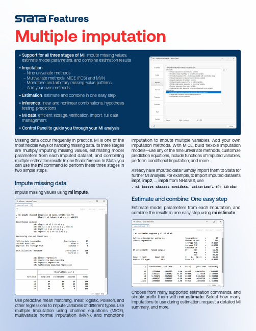
Multiple imputationEstimate model parameters from each imputation, and combine the results in one easy step using mi estimate .Choose from many supported estimation commands, and simply prefix them with mi estimate . Select how many imputations to use during estimation, request a detailed MI summary, and more.Missing data occur frequently in practice. MI is one of the most flexible ways of handling missing data. Its three stages are multiply imputing missing values, estimating model parameters from each imputed dataset, and combining multiple estimation results in one final inference. In Stata, you can use the mi command to perform these three stages in two simple steps.Use predictive mean matching, linear, logistic, Poisson, and other regressions to impute variables of di erent types. Use multiple imputation using ch ained equations (MICE), multivariate normal imputation (MVN), and monotoneImpute missing values using mi impute .• Support for all three stages of MI: impute missing values,estimate model parameters, and combine estimation results • Imputation– Nine univariate methods– Multivariate methods: MICE (FCS) and MVN – Monotone and arbitrary missing-value pa erns – Add your own methods • Estimation : estimate and combine in one easy step • Inference : linear and nonlinear combinations, hypothesis testing, predictions• MI data : e cient storage, verification, import, full data management• Control Panel to guide you through your MI analysis imputation to impute multiple variables. Add your own imputation methods. With MICE, build flexible imputation models—use any of the nine univariate methods, customize prediction equations, include functions of imputed variables, perform conditional imputation, and more.Already have imputed data? Simply import them to Stata for further MI analysis. For example, to import imputed datasets imp1, imp2, ..., imp5 from NHANES, use. mi import nhanes1 mymidata, using(imp{1-5}) id(obs)Impute missing dataEstimate and combine: One easy step© 2023 StataCorp LLC | Stata is a registered trademark of StataCorp LLC, 4905 Lakeway Drive, College Station, TX 77845, USA./multiple-imputationA er estimation, for example, perform hypothesis testing.At any stage of your analysis, perform data management as if you are working with one dataset, and mi will replicate the changes correctly across the imputed datasets. Stata o ers full data management of MI data: create or drop variables and observations, change values, merge or append files, add imputations, and more.Accidentally dropped an observation from one of the imputed datasets, or changed a value of a variable, or dropped a variable, or ...? Stata verifies the integrity of your MI data each time the mi command is run. (You can also do this manually by using mi update .) For example, Stata checks that complete variables contain the same values in the imputed data as in the original data, that incomplete variables contain the same nonmissing values in the imputed data as in the original,and more.If an inconsistency is detected, Stata tries to fix the problem and notifies you about the result.Estimate transformations of coe cients, compute predictions, and more.Stata’s mi command uniquely provides full data management support, verification of integrity of MI data at any step of the analysis, and multiple formats for storing MI data e ciently. And you can even add your own imputation methods!Use an intuitive MI Control Panel to guide you through all the stages of your MI analysis—from examining missing values and th eir pa erns to performing MI inference. Th e corresponding Stata commands are produced with every step for reproducibility and, if desired, later interactive use.Stata o ers several styles for storing your MI data: you can store imputations in one file or separate files or in one variable or multiple variables. Some styles are more memory e cient, and others are more computationally e cient. Also, some tasks are easier in specific styles.You can start with one style at the beginning of your MI analysis, for example, “full long”, in which imputations are saved as extra observations:. mi set flongIf needed, switch to another style during your mi session, for example, to the wide style, in which imputations are saved as extra variables:. mi convert wideCan’t find an imputation method you need? With li le e ort, you can program your own. Write a program to impute your variables once, and then simply use it with mi impute to obtain multiple imputations.program mi_impute_cmd_mymethod... program imputing missing values once ...end. mi impute mymethod ..., add(5) ...Manage imputed dataMultiple storage formatsAdd your own imputation methodsVerify imputed dataInferenceIn addition...Control Panel。
plire方法

plire方法PLIRE方法是一种新兴的、高效的机器学习算法,被广泛应用于数据挖掘、文本分类、图像识别等领域。
本文将详细介绍PLIRE方法的原理、特点以及应用场景,帮助读者更好地理解和掌握这一方法。
一、PLIRE方法简介PLIRE(Pattern Learning with Imbalanced Ratio Estimation)方法是一种针对类别不平衡问题的机器学习方法。
在实际应用中,我们经常会遇到类别不平衡的问题,即不同类别的样本数量差异较大。
这会导致传统分类算法在训练过程中过分关注多数类,而忽视少数类,从而降低分类性能。
PLIRE方法通过估计类别不平衡比例,自适应地调整分类器的学习策略,使得分类器在训练过程中能够更好地关注少数类,提高分类性能。
二、PLIRE方法原理1.类别不平衡比例估计PLIRE方法首先对训练数据进行类别不平衡比例估计。
具体地,它采用了一种基于密度估计的方法,通过计算每个类别的密度函数,得到类别不平衡比例。
2.样本权重调整根据类别不平衡比例,PLIRE方法对训练样本进行权重调整。
对于少数类的样本,增加其权重;对于多数类的样本,减少其权重。
这样,分类器在训练过程中会更加关注少数类。
3.模式学习在权重调整后的训练数据上,PLIRE方法采用一种基于模式的学习策略。
它通过提取具有区分性的模式,构建分类器。
这些模式可以是特征组合、原型样本等。
4.分类器融合PLIRE方法通过集成多个分类器,提高分类性能。
这些分类器可以是基于不同模式学习策略的,也可以是不同参数设置下的同一分类器。
三、PLIRE方法特点1.自适应调整权重:PLIRE方法根据类别不平衡比例,自适应地调整样本权重,使分类器更好地关注少数类。
2.模式学习:PLIRE方法通过提取具有区分性的模式,构建分类器,提高分类性能。
3.集成学习:PLIRE方法采用多个分类器进行融合,进一步提高分类性能。
4.适用性广:PLIRE方法适用于多种类型的机器学习任务,如文本分类、图像识别等。
选择与坚持:跨期选择与延迟满足之比较

第2期
任天虹等 : 选择与坚持:跨期选择与延迟满足之比较
305
会通过预实验选择一对较为恰当的 SS 与 LL, 以 保证 SS 与 LL 之间的差异既要大到足以使被试愿 意选择后者 , 又要小到使 SS 对儿童有足够的诱惑 , 从而避免等待时间的天花板效应与地板效应 (Mischel & Underwood, 1974)。 动物实验在跨期选择与延迟满足的研究中都 有 所 涉 及 , 这 些动 物研 究 的 实验 范式 直 观 易 懂 , 对儿童被试的研究也颇有启示意义。随着研究内 容的扩展与研究范式的改进 , 跨期选择与延迟满 足在研究对象上有融合的趋势。 3.2 研究内容 跨期选择关注被试的时间折扣 (time discounting), 而延迟满足则更关注被试在等待时间上的 个 体 差 异 、 自 我 控 制 策 略 及 其 有 效 性 (Ainslie, 1975; Mischel et al., 1989)。如果说跨期选择的研 究者将其研究重点放在了计算、分析、推理、权 衡等较为高级的认知过程上 , 那么延迟满足的研 究者则将其重点放在了情绪、意志力、动机强度 等更为基础的本能反应上。 时间折扣是跨期选择研究的基本假设 , 也是 其研究的重要内容 , 它是指在跨期选择中 , 个体 首先会对延迟结果的价值根据其延迟的时间进行 一定的折扣, 然后再对两个结果进行比较(Frederick et al., 2002; Scholten & Read, 2010)。经济学家力 图找到某一通用的公式来描述折扣程度与结果及 延 迟 时 间 之间 的 关 系 , 表 现 为 数 理 模 型 的 优化 ; 心理学家则更关注外界因素对个体时间折扣程度 的影响 , 表现为认知神经机制的揭示。 延迟满足的研究者并不关注折扣程度 , 他们 更加关注等待时间上的个体差异 , 并在实验中细 致地检验被试自我控制策略的选择与使用状况 , 这些研究者热衷于以追踪研究揭示儿童在实验中 的表现与其个性及行为特征之间的关系 (Mischel et al., 1989)。 3.3 研究范式 跨期选择的研究关注被试的选择过程 , 它要 求被试做出一系列选择 ; 延迟满足则更关注被试 的坚持过程 , 要求被试坚持完成选择后的等待过 程。尽管在跨期选择的部分任务中也涉及到等待 过程 , 但是它与延迟满足有本质的区别。被试在 延迟满足任务中能够自主选择中止等待 , 而在跨 期选择任务中则只能消极等待延时结束 (Evans & Beran, 2007)。
基于两层BiLSTM的问题回答技术研究

基于两层BiLSTM的问题回答技术研究随着人工智能技术的不断发展,自然语言处理技术也得到了长足的进步。
问题回答技术作为自然语言处理的重要分支之一,一直受到了广泛的关注和研究。
在问题回答技术研究中,基于两层BiLSTM的模型逐渐成为了研究热点,该模型不仅可以捕捉语境信息,还可以对输入语句进行双向建模,从而提高了问题回答的准确性和效率。
本文将针对基于两层BiLSTM的问题回答技术进行深入研究和分析,首先将介绍BiLSTM模型的基本原理和特点,然后探讨基于两层BiLSTM的问题回答模型的结构和优势,最后将对该模型在问题回答任务中的应用进行实例分析。
通过本文的研究,希望能够更深入地理解基于两层BiLSTM的问题回答技术,并为相关领域的研究和实践提供一定的参考。
一、 BiLSTM模型的基本原理和特点BiLSTM(Bidirectional Long Short-Term Memory)即双向长短期记忆网络,是一种基于循环神经网络(RNN)的模型,其主要特点是能够对输入序列进行双向建模,从而充分捕捉上下文信息。
在自然语言处理任务中,BiLSTM模型通常用于处理文本序列,如文本分类、命名实体识别和情感分析等任务。
BiLSTM模型由两个方向的LSTM单元组成,分别对输入序列进行前向和后向的建模。
通过前向和后向两个方向的信息传递,BiLSTM模型能够准确地理解输入序列的语境信息,从而有效地提高模型的性能和效果。
BiLSTM模型还可以避免信息丢失和梯度消失的问题,使得模型在处理长文本序列时依然能够保持较好的表现。
二、基于两层BiLSTM的问题回答模型结构和优势在传统的基于两层BiLSTM的问题回答模型中,通常包括了输入层、编码层、匹配层和输出层。
输入层用于接收问题和答案的输入向量,编码层通过两个独立的BiLSTM网络分别对问题和答案进行编码,匹配层则用于计算问题和答案之间的相似度,最后通过输出层给出最终的回答结果。
提示工程(prompt)

客户问题:{在此插入新问题} 分类主题:
之前
单个家庭的年用水需求是多少? 包含四个在家的人的家庭 每年平均200天,使用量平均为100 每天多少升水?
单户家庭的年用水需求 包含四个人,他们平均在家的时间为 每年200天,平均使用100升的 每天的用水量为每年800万升。
2nd prompt—答案提取
一个普通人在一分钟内能打出25拳。 一场比赛持续5个回合,每回合3分钟。有多少 他投掷了多少拳?
让我们一步一步地思考并解释这个计算过程。 一步一步地 。
在一分钟内,乔打了25拳。
在三分钟内,乔打了3 * 25 = 75拳。
在五轮中,乔投掷了5*75 = 375次拳。
在一分钟内,乔打了25拳。 在三分钟内,乔打了3 * 25 = 75拳。 在五轮中,乔投掷了5*75 = 375次拳。
提示链
摘要
请总结信息 关于产品 [{'text': 'iPhone', 'type': '产品'}], {'text': '苹果', 'type': 'ORGANIZATION’}]
iPhone是一系列智能手机。 由苹果设计并销售 Inc. 这些设备结合了 计算机、相机和互联网 单一设备中的连接性,以及 以其简洁的设计而闻名 用户友好的界面。
人工智能 机器学习 深度学习
生成式人工智能
1956
人工智能
计算机科学领域中致力于创造的分支 能够复制或超越人类智能的智能机器 人类智能
1997
机器学习
人工智能的子集,使机器能够从 现有数据,并在该数据的基础上进行改进,以使其 决策或预测
- 1、下载文档前请自行甄别文档内容的完整性,平台不提供额外的编辑、内容补充、找答案等附加服务。
- 2、"仅部分预览"的文档,不可在线预览部分如存在完整性等问题,可反馈申请退款(可完整预览的文档不适用该条件!)。
- 3、如文档侵犯您的权益,请联系客服反馈,我们会尽快为您处理(人工客服工作时间:9:00-18:30)。
DesignCon 2010Predicting BER with IBIS-AMI: experiences correlating SerDes simulations and measurement Todd Westerhoff, Signal Integrity Software, Inc. twesterh@Adge Hawes, IBMadge@Dr. Michael Steinberger, Signal Integrity Software, Inc. msteinb@Kent Dramstad, IBMDramstad@Dr. Walter Katz, Signal Integrity Software, Inc.wkatz@Barry Katz, Signal Integrity Software, Inc.bkatz@AbstractThe IBIS A lgorithmic M odeling I nterface (IBIS-AMI) allows SerDes vendors to provide simulation models that run in multiple simulation environments. This has created the market for commercial SerDes channel simulators and raised the question of how well IBIS-AMI models correlate to both SerDes vendor internal simulation tools and hardware measurements. This paper presents the results of a three-year effort to develop and correlate IBIS-AMI models for IBM’s family of SerDes cores. The correlation methodology and results for simulator-to-simulator correlations are presented. Author BiographiesTodd Westerhoff, Vice President of software products for SiSoft, has over 30 years experience in the modeling and analysis of electronic systems, including 14 years of signal integrity experience. Prior to joining SiSoft, Todd managed a high-speed design group that provided static timing, signal integrity and design rule consultation to various ASIC and system engineering groups within Cisco. Previously, Todd was the SPECCTRAQuest Product Manager for Cadence Design Systems and a signal integrity consultant to a number of Fortune 500 companies. He has held product marketing positions at Compact Software, Racal-Redac, FutureNet and HHB-Systems. Todd holds a B.E. degree in Electrical Engineering from the Stevens Institute of Technology in Hoboken, New Jersey.Adge Hawes is a Development Architect for IBM at its Hursley Labs, United Kingdom. He has worked for IBM for more than 30 years across such hardware as Graphic Displays, Printing Subsystems, PC development, Data Compression, and High-Speed Serial Links. He has represented the company in many standards bodies such as PCI, SSA, ATA, Fibre Channel and IBIS. He now develops simulators for IBM's High Speed Serial Link customers. He received a BSc (Hons) Electronics from Southampton University (UK) in 1976.Dr. Michael Steinberger is currently responsible for leading the development of SiSoft's serial link analysis products. He has over 30 years experience in the design and analysis of very high speed electronic circuits. Prior to joining SiSoft, Dr. Steinberger worked at Cray Inc., where he designed very high density interconnects and increased the data rate and path lengths to the state of the art. Mike holds a B.S. from the California Institute of Technology and a Ph.D. from the University of Southern California, and has been awarded 13 U.S. patents.Kent Dramstad is an ASIC Application Engineer at IBM. A 1980 BSEE graduate of Iowa State University, he has over 29 years of experience working on both power and signal integrity issues for a wide variety of applications. His current emphasis is on helping customers select and integrate IBM’s series of High Speed Serdes (HSS) cores into their ASIC designs.Dr. Walter Katz, Chief Scientist for SiSoft, is a pioneer in the development of constraint driven printed circuit board routers. He developed SciCards, the first commercially successful auto-router. Dr. Katz founded Layout Concepts and sold routers through Cadence, Zuken, Daisix, Intergraph and Accel. More than 20,000 copies of his tools have been used worldwide. Dr. Katz developed the first signal integrity tools for a 17 MHz 32-bit minicomputer in the seventies. In 1991, IBM used his software to design a 1 GHz computer. Dr. Katz holds a PhD from the University of Rochester, a BS from Polytechnic Institute of Brooklyn and has been awarded 5 U.S. Patents.Barry Katz, President and CTO for SiSoft, founded SiSoft in 1995. As CTO, Barry is responsible for leading the definition and development of SiSoft’s products. He has devoted much of his efforts at SiSoft to delivering a comprehensive design methodology, software tools, and expert consulting to solve the problems faced by designers of leading edge high-speed systems. He was the founding chairman of the IBIS Quality committee. Barry received an MSEE degree from Carnegie Mellon and a BSEE degree from the University of Florida.IntroductionThe IBIS A lgorithmic M odeling I nterface (IBIS-AMI) provides a standardized way of modeling the behavior of multi-Gigabit SerDes transceivers for serial link simulations. The first question users ask about any new simulation model is usually “is it accurate?” To provide an objective and meaningful answer, it’s important to qualify exactly what constitutes acceptable accuracy and how it is measured.IBIS-AMI models are typically compared to two different references:•Simulation results from other simulation tools•Hardware measurementsThis paper describes the process used to develop and correlate IBIS-AMI models for IBM’s family of High Speed SerDes (HSS) transceiver cores. In practice, answering the question “is it accurate?” requires defining a set of specific correlation test cases, metrics and criteria. The correlation metrics need to be defined based on the reference source (hardware measurement or other simulator) and based on which aspects of device behavior can be reliably controlled and observed.SerDes analysisSerial link simulation requires different tools and techniques than traditional parallel interface signal integrity analysis. Serial links typically look to achieve bit error rates of fewer than 1 in every 1E15 bits. Predicting operating margins at these low probability levels requires simulating a million bits (or more) to adequately characterize the effects of Duty Cycle Distortion (DCD) and Inter-Symbol Interference (ISI). Simulation results are post-processed to account for the effects of different noise and jitter sources, which allows prediction of operating margins at very low probability levels.IBM’s High Speed SerDes / Clock Data Recovery (HSSCDR) simulator is a proprietary MATLAB based system-level signal integrity simulator that support’s IBM’s HSS cores. HSSCDR uses behavioral models of the IBM HSS I/O circuits along with S parameter descriptions of the individual components in the serial data path to provide a very fast, robust means of predicting signal quality on high-speed channels. HSSCDR provides greatly reduced simulation times compared to extracted element models (such as HSPICE). HSSCDR can also provide optimized control settings (pre-emphasis, output power, receiver amplification, receiver equalization, etc.) for peak signal quality performance with different customers’ individual link characteristics.IBM correlates HSSCDR simulations against hardware measurements for each new generation of HSS cores to ensure that simulations correctly predict the behavior exhibited by the hardware. This allows customers building serial links using IBM ASICs to predict the behavior of a proposed system implementation before manufacture, adjusting both the system design and SerDes settings to optimize operating margin. This process works well when IBM silicon is employed at both ends of the link, but what happens when another vendor’s silicon is used on one end of the link?HSSCDR is a dedicated simulation environment based on IBM technology; there are no provisions for plugging a model for another vendor’s silicon into HSSCDR. That’s where IBM’s IBIS-AMI models come into play.IBIS-AMIIBIS-AMI is part of the IBIS 5.0 standard and defines a method for modeling SerDes analog I/O characteristics, equalization and clock recovery behavior. IBIS-AMI was developed by a consortium of EDA, Semiconductor and Systems companies beginning in 2006 and was adopted as part of IBIS 5.0 in August, 2008.The design goals established for IBIS-AMI were:•Interoperability – Models from different semiconductor vendors run together in the same simulation•Transportability – The same model runs in different simulators•Performance – IBIS-AMI based simulation should provide comparable performance to a semiconductor vendor’s proprietary simulator •Accuracy – IBIS-AMI based simulations should provide results comparable to those obtained with proprietary semiconductor vendor tools•IP Protection – Semiconductor vendors need to be able to provide accurate models of their devices without divulging internal architectural details.IBIS-AMI models must allow semiconductor vendors to control how much, orhow little detail is exposed to the userIBIS-AMI assumptions and terminologyMany channel simulators (HSSCDR included) accept a model for the serial channel as S parameter data. The channel can be described as a single S parameter block or as a cascaded set of blocks, but in either case, the user input to the simulator represents the passive (unpowered) portion of the channel. The models for the transmitter’s equalization and output driver, receiver termination network, receiver equalization and clock recovery have traditionally been built directly into the channel simulator.IBIS-AMI makes the assumption that transmitter equalization is electrically isolated (buffered) from the channel, such that variations in channel loading don’t affect the input signal presented to the transmitter’s output driver. The same assumption is made at the receiver – changes in equalization or clock recovery behavior don’t affect the input signal at the receiver die pad.The IBIS-AMI specification states this assumption using the following language:“The transmitter equalization, receiver equalization and clock recovery circuits are assumed to have a high-impedance (electrically isolated) connection to the analog portion of the channel. This makes itpossible to model these circuits based on a characterization of the analog channel.”IBIS-AMI treats the analog channel as linear and time-invariant (LTI). The analog channel is “characterized” using circuit analysis techniques, and that characterization data (in the form of an impulse response) is combined with models of the SerDes equalization and clock recovery behavior to predict the overall behavior of the link.The assumption that the analog channel can be characterized is key to increasing simulation speed and being able to simulate the millions of bits needed to predict serial link behavior.IBIS-AMI uses the following terms to describe portions of a serial link:Figure 1: IBIS-AMI passive channel•The passive channel is defined as all the passive, unpowered interconnect between the transmitter and receiver pads. This includes device packages, vias,PCB etch and cables.Figure 2: IBIS-AMI analog channel•The analog channel combines the passive channel with the transmitter’s analog output section and the receiver’s input termination network. This is the part ofthe link that is assumed to be electrically isolated from the equalization and clock recovery circuitry.Figure 3: IBIS-AMI end to end channel•The end to end channel combines the analog channel (represented as an impulse response) with algorithmic models for TX / RX equalization andRX clock recovery.IBIS-AMI based analysisIBIS-AMI simulation occurs in two stages: Network Characterization and Channel Simulation.Network Characterization uses circuit analysis techniques to characterize the analog channel and derive its impulse response. Network Characterization uses a model of the passive channel and models of the SerDes TX / RX analog characteristics to perform this analysis.Channel Analysis takes the impulse response created by Network Characterization and uses Algorithmic Models for the TX / RX equalization and clock recovery to simulate the link’s end to end behavior. Channel simulators are a new breed of tool - they don’t perform circuit analysis the way SPICE does. Instead they use communications analysis techniques (data sampling, interpolation & convolution) to perform Statistical andTime-Domain simulation.Channel Analysis comes in two forms:•Statistical simulation produces an eye diagram showing the probabilities of signal distribution at the receiver, but doesn’t use a specific stimulus sequence.Statistical analysis has the advantage of being very fast (individual simulationsonly take a second or so), but makes the assumption that the TX / RX equalization behavior is linear and time-invariant. In practice, this means that Statisticalsimulation can be used to approximate Decision Feedback Equalizer (DFE) andclock recovery behavior, but more detailed models are needed to fully validate the link’s behavior.•Time-Domain simulation behaves much like traditional SPICE-based analysis in the sense that an input stimulus is applied and a waveform representing thecircuit’s behavior is generated. The difference is speed – IBIS-AMI basedTime-Domain analysis typically runs at a million bits per minute. This form ofanalysis is suitable for modeling the adaptive behavior of DFE control loops andclock recovery circuitry.IBIS-AMI modelsGiven that IBIS-AMI based simulation occurs in two stages, it should come as no surprise that IBIS-AMI models are supplied in two parts – an analog model used for Network Characterization and an algorithmic model used for Channel Analysis. The combination of these two models represents the complete behavior of the device.The analog portion of an IBIS-AMI model contains the information a simulator needs to determine the impulse response for the channel when equalization is turned off. From a practical standpoint, the elements of the analog model are:•Transmitter: output voltage swing, impedance, slew rate, output parasitics•Receiver: input termination network impedance & parasiticsThe algorithmic model is a behavioral model supplied as executable code that gets linked into the channel simulator at run time. IBIS-AMI defines the calling interface between the simulator and the model linked into it. Providing models as executable code maximizes simulation speed, which was one of the design goals for IBIS-AMI.IBIS-AMI algorithmic models can support two different levels of processing: •Impulse response processing – an impulse response is passed to the algorithmic model, which applies its equalization and passes back a modified impulseresponse. This level of modeling is ideally suited to Statistical simulation, butcan also be used for Time-Domain simulation.•Waveform processing – a waveform is passed to the algorithmic model, which applies its equalization and passes back a modified waveform. If the algorithmic model represents a receiver, the model can also pass back clock ticks thatrepresent the output of the receiver’s clock recovery algorithm. This level ofmodeling can only be used by Time-Domain simulation.Algorithmic models are accompanied by a text control (.AMI) file that tells the channel simulator which processing modes the model supports and lists any model-specific control parameters. Model-specific control parameters allow users to configure the behavior of the model to emulate the way the hardware is programmed.HSSCDRDesigners simulate their channels in HSSCDR by providing an S parameter model of their channel from package pin to package pin. HSSCDR includes models for IBM’s SerDes cores and device packages. Users specify which device technology is to be used and how hardware options are to be configured, and HSSCDR provides simulation results for how IBM’s devices with work with the customer’s channel.HSSCDR performs high-performance Time-Domain simulation, with a throughput of about 500K bits/minute. Simulation results are post-processed to account for the effects of TX / RX jitter and other random noise sources. Statistical post-processing & extrapolation are performed automatically, predicting link operating margins at probability levels down to 1E-15 based on simulation runs of 1M bits.IBM’s IBIS-AMI modelsDeveloping models for all the SerDes cores represented in HSSCDR is a daunting task – HSSCDR currently supports more than 17 different sets of SerDes cores implemented across 5 different process nodes. Models for IBM’s SerDes cores are referenced in HSSCDR by speed and process node. Control files in HSSCDR configure the simulation algorithms built into the simulator for the technology being modeled.IBM’s strategy for developing IBIS-AMI models mirrors the way HSSCDR operates. A central set of modeling algorithms is implemented in a common set of algorithmic models, which use configuration data specific to each speed and process node to configure themselves. The .AMI control file supplied with IBM’s algorithmic models supplies the data for this task.The .AMI file configures the algorithmic model to provide the correct number of equalization taps for the technology being modeled, sets the maximum limits for each tap and configures the capabilities of the receiver’s Automatic Gain Control (AGC) and DFE behavior. The .AMI file declares the sensitivity of the receiver’s sampling circuit, so the simulator can determine whether enough voltage has been developed at the sampling point to allow error-free operation.The models also use the .AMI file to declare model parameters users can control through the simulator’s graphical interface. The names and settings of these parameters correspond as closely as possible to their HSSCDR equivalents, allowing existing HSSCDR users to leverage their existing settings for IBIS-AMI use.Figure 4: Control parameters exposed by IBM IBIS-AMI modelsIBM characterizes the transmitter analog output and receiver termination network over a wide frequency range to determine signal transmission and reflection characteristics. IBM captures this information in S parameter format and HSSCDR uses this data to model how the analog portions of the transmitter and receiver interact with the channel. The IBIS 5.0 specification provides methods for modeling analog I/O that have worked well for lower speed parallel interface applications, but which don’t capture the frequency-dependent behavior needed for serial link analysis. The results presented in this paper are based on using IBM’s on-die S parameter data to provide the analog model characteristics. Extending the current IBIS-AMI specification to allow use ofS parameter data has been proposed as an extension to IBIS-AMI by IBM, SiSoft and Cisco. More information on this proposal can be found in [5].Correlation BackgroundComplete correlation between simulators or between simulation and hardware is an obvious goal, but determining what level of correlation is acceptable, and under what conditions – is essential to success. 100% correlation between any two channel simulators is highly unlikely, and perfect correlation to hardware measurement is impossible, because even two repeated hardware measurements can’t be expected to match precisely.To be able to achieve correlation, one must define:•What is going to be compared to what?•Under what conditions?•What can be controlled & what can’t?•What metrics will be used and what level of correlation is expected?It’s also important to note that correlating simulator to simulator and simulator to hardware are two different activities. Correlating simulation to hardware presents one set of challenges:•Observability at the SerDes sampling latch is limited and depends on the receiver in question•Controllability (stimulus, ability to set tap coefficients, etc) depends on the hardware under test•Some behaviors (random jitter, etc) can’t be controlled or isolatedCorrelating between simulation environments presents a different set of challenges: •Different simulators will have different inputs and outputs•Post-processing & extrapolation details are simulator-specific (and in the case of HSSCDR, proprietary)Correlation MethodologyFor this project, correlation between simulators was pursued first because the results from each simulation tool were repeatable and because HSSCDR has already been extensively correlated to hardware. It might seem that correlating two simulators would be straightforward – running simulations in both tools and comparing the resulting waveform output. In actual practice, running million bit simulations and comparing waveforms proved to be neither practical nor particularly insightful.The end goal of the IBIS-AMI correlation effort was to reproduce the horizontal (timing) and vertical (voltage) eye margins as reported by HSSCDR. We identified all the different model elements, simulation and post-processing that factor into this computation (Figure 5) and defined a process that would allow us to correlate all of these factors in a controlled manner.Figure 5: Factors in computing eye marginsThe simulator correlation methodology we used was:1.Assess the different simulator input / outputs first, determine what can becontrolled / compared and how2.Start with as simple a simulation as possible and add complexity incrementally3.Correlate after each new behavior is added4.Add jitter & noise modeling into the analysis only after TX / Channel / RXmodels were correlated5.Correlate post-processing & extrapolation algorithms lastCorrelation of IBIS-AMI models to hardware measurement is the next stage of this project; publishable results were not available at the time this paper was written.IBIS-AMI to hardware correlation will follow the same path IBM uses to correlate HSSCDR to hardware. This approach leverages hardware measurements and correlation data IBM already has available.In all cases, correctly setting expectations is key to success. For simulator to simulatorcorrelation, the goal was to match HSSCDR’s predicted operating margins within 5%.Simulator comparisonCorrelation would be easier if both simulators had the same inputs and outputs, but they don’t. Channel simulators are their own breed of tool; since they simulate millions of bits worth of information, they necessarily accumulate, post-process and summarize data for presentation.HSSCDRHSSCDR takes a channel model as input, specified as S parameter data. The user specifies the data rate, input pattern type, device technology (e.g. Cu045 HSS12), package selection and other settings via a graphical interface. Simulation models for the different IBM technologies and packages are supplied as part of HSSCDR. When the simulation is complete, the GUI presents a collection of plots (Log BER, Impulse Response, Transfer Function, Eye Diagram & Eye Height) that display results from the simulation.Figure 6: HSSCDR OuputsHSSCDR also provides a text output report that lists eye margins at different probability levels. A section of this report is shown below:HMIN -37.5% HMAX 34.0% HEYE 68.1% 10^-3HMIN -37.5% HMAX 32.8% HEYE 65.6% 10^-6HMIN -37.5% HMAX 32.8% HEYE 65.6% 10^-9HMIN -37.5% HMAX 32.8% HEYE 65.6% 10^-12HMIN -37.4% HMAX 32.8% HEYE 65.6% 10^-15BER FLOOR = 1.0e-300VMIN 64.7% VMAX 125% VEYE 65.8mV 10^-3VMIN 63.2% VMAX 129% VEYE 64.2mV 10^-6VMIN 62.9% VMAX 129% VEYE 63.9mV 10^-9VMIN 62.8% VMAX 130% VEYE 63.8mV 10^-12VMIN 62.6% VMAX 130% VEYE 63.6mV 10^-15Figure 7: HSSCDR text output reportThe text report proved to be the best metric for comparing simulation results for the end to end channel, because it represented the simulation data accumulated over the entire simulation run and included the projected effects of jitter and random noise over large numbers of patterns. Remember that the channel simulator is typically only simulating millions of bits, while a typical target channel bit error rate might be 1 in every 1E15 bits or more. Predicting link margins requires combining simulated data with extrapolated data to predict link margins at the probability levels the user ultimately cares about. HSSCDR also records “raw” waveform data to a binary file, which can be displayed in a waveform viewer. The challenge is that the “raw” waveform data doesn’t include the effects of RX equalization and clock recovery. Thus, the “raw” waveform data is useful for correlating everything up to the RX pad, but not for correlating past that point in the channel.The HSSCDR outputs used for this study are outlined in red in Figure 6.Quantum Channel DesignerSiSoft’s Quantum Channel Designer (QCD) is a commercial channel simulator that can use either HSPICE or IBIS-AMI models for simulation. In this study, the IBM transmitter and receiver were supplied as IBIS-AMI models.The channel model to be analyzed in QCD is captured graphically, and can consist of a mixture of S parameter blocks, lossy transmission lines, SPICE subcircuits and individual R/L/C elements. The user specifies the stimulus pattern, data rate & model control parameters via the graphical interface.In this study, the same S parameter channel and package data was used in both simulators.Quantum Channel Designer has two simulation modes: a Statistical simulation mode that uses convolution techniques to analyze the effects of very large populations (>10**100) of random bit sequences, and a Time-Domain simulation mode that analyzes the effects of specific input sequences. Statistical simulation requires linear (impulse response processing) models for transmit / receive equalization, while Time-Domain simulation makes use of non-linear, time-varying (waveform processing) models. QCD’sTime-Domain mode most closely resembles HSSCDR, and the QCD results in this study were derived from Time-Domain simulation.Figure 8: Quantum Channel Designer (QCD) output plotsQCD provides a collection of output plots, including impulse / pulse / step responses, waveform plots, eye diagrams, data bathtub & clock PDF plots, network transfer functions and eye plots color coded to show signal distribution. QCD also computes and displays a number of metrics, including channel & reflection loss, projected BER, and eye height / width at a number of different probability levels. The QCD outputs used for this study are outlined in red in Figure 8.Correlation MetricsWe needed data from the two different simulation environments that could be readily compared and was also statistically significant. After analyzing the different outputs from each tool, we defined the following basis for comparison:•“Raw” waveform data from HSSCDR could be compared against waveform plots in QCD to correlate everything up to and including the RX pad•The HEYE / VEYE margin data from HSSCDR’s text output report could be compared against the corresponding Contour Plot measurements from QCDComparing the “raw” waveform data from HSSCDR against waveforms produced in QCD is a direct method and has the advantage that many data points (the voltage of the signal at each point in time) are available for comparison. It’s easy to overlay waveforms and assess the quality of the result, and it’s usually obvious when something is wrong. Comparing eye voltage and timing margins from simulation is an indirect method, requiring the simulator to first combine the simulated data & recovered clock behavior to derive eye statistics and contours, then measuring the eye height and width. The conundrum with this measurement is that although many bits are represented, the number of actual data points for comparison is small. We measured at probability levels from1E-3 to 1E-15, providing 5 data points each for voltage and timing margin. With fewer data points for comparison, more simulations and channels needed to be studied to ensure the consistency of the results..We created a set of test cases that started as simple as possible and allowed us to introduce and correlate new behaviors in a controlled fashion. We zeroed out the effects of jitter & noise until after we were sure we had the transmitter / channel / receiver modeling correlated.As these simulations were something we expected to repeat many times before the study was done, we automated as much of the process as possible.Correlation cases and resultsTransmitter CorrelationIn all of the waveforms that follow, the blue waveforms show HSSCDR results and the red waveforms show QCD results. The IBM waveforms are “in front” – where the red waveforms aren’t visible, they’re completely hidden behind the HSSCDR results.The first (and simplest) test cases consisted of a transmitter driving directly into a resistive load without a package model. Using such a simple test case allowed us to correlate drive levels, slew rates and equalization characteristics of the transmitter model directly.Figure 9: HSSCDR / QCD waveforms for simple TX case。