ANSYS13.0理论参考手册
ANSYS ICEM 13.0 Tutorial mannual中文翻译
ICEM Tutorial Manual2D Pipe Junction1.1准备1.1.1 从ANASYS安装目录里拷贝输入几何文件(geometry.tin),v130/icemcfd/samples/CFD_Tutorial_files/2DPipeJunct。
1.1.2 打开ANSYS ICEM CFD并打开几何(geometry.tin)。
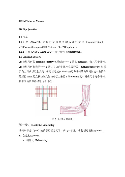
1.2 Blocking Strategy2D管道几何的blocking strategy包括创建一个T形的blocking并将其用于几何。
2D管道几何相当于一个T形。
右边的非阻塞交叉开关(blocking crossbar)仅需要向上弯曲以组装几何。
你可以通过在block的边和几何的曲线间创建一些附件然后将block的点移动到几何的角落上来将T形blocking的材料应用于这个几何。
接下来的步骤将描述这个过程。
图2. 网格及其拓扑第一步:Block the Geometry几何和部分(part)的信息已经定义了。
在这一步里,你将创建最初的block。
1.创建初始block。
a.初始化2D blockingi.在Part区域中输入FLUID。
ii.在Type下拉菜单中选择2D Plannar。
iii.点击Apply。
b.在Blocking下激活Vertices。
c.在Vertices下选择Numbers。
将blocking下面的Vertices前面的方框勾选,右击,在弹出菜单中选择Numbers即可。
图2给出了包裹几何的初始block。
你将使用这个初始block来创建这个模型的拓扑。
图3. 初始block这些曲线现在被分别上色,并不是由不同部分。
这样可以使你区别不同的曲线实体,这对于某些blocking操作时非常必要的。
你可以通过选择/不选Show Composite激活或者不激活上色命令。
2.将初始block分割为次级block。
本案中,你将使用两个垂直分割和一个水平分割将初始block分割。
ANSYS13.0安装及破解指南(图文)

ANSYS13.0安装及破解指南(图文)ANSYS 13.0安装及破解指南1.首先要确保系统已经安装有虚拟光驱软件。
雨菲的机器安装有Deamon Tools Lite,就以之为例。
2.在Deamon Tools Lite中加载ANSYS文件夹中的两个ISO镜像文件3.选择两个镜像中的A光盘,文件名为[ANSYS.13.0].[ANSYS.13.0].[ANSYS.13.0].[ANSYS.13.0].m-a1332a.iso并点击绿色的三角形按钮载入虚拟光驱4.如果系统有光盘自动播放的功能,就会自动弹出来对话框,我们要选择“运行setup.exe”,如果光盘没有自动运行,我们需要手动打开我的电脑,进入虚拟光驱盘,在根目录下找到“setup.exe”并执行(Vista或Win7用户建议右键点击图标,选择“以管理员身份运行“之后讲出现ANSYS安装的选项,如图所示5.我们选择第一项“Install ANSYS“开始安装ANSYS,可以看到许可界面,依然是同意,不解释6.这时出现的是安装选项,首先选择安装的路径,随便写,由于软件比较大,不推荐安装到C盘。
下面有两个选择框,建议都选中,打上勾。
7.这里看到的是安装功能的选择。
反正我们用破解的,而且也不差啥硬盘空间,就都选择打上勾吧~8.这里要填一些信息,由于我们木有这些信息,也就不用造假了,底下有两个SKIP的选项,都选中打上勾,然后果断下一步9.又是一个填信息的,果断依然两个全SKIP,然后下一步10.这是最后一个了,我们还是不填,选中SKIP然后点击下一步11.这里要选择一些配置,我们不管,依然是SKIP,然后就下一步(终于要正式安装了)12.它要检查点啥东西吧,不管,直接下一步13.在安装之前它把配置列出来,让你看看,这时候还可以反悔奥14.进入了漫长的等待,我的心在等待,在啊在等待哎哎。
15.67个文件解压缩完毕之后提示要换光盘了,就像有的大型游戏得有A盘B盘似的,我们在DeamonTools Lite中加载B光盘就可以了,然后依旧是点击那个绿色的小三角,然后在ANSYS的安装界面直接确定就可以16.惊奇地发现居然还有40个要解压的。
ANSYS WorkBench 13.0从入门到精通

1.5.7 施加载荷 与约束
A
1.5.8 结果后处 理
B
1.5.9 保存与退 出
C
1 初识ANSYS Workbench 13.0
1.5 Workbench实例入门
02
2 创建Workbench几何模型
2 创建Workbench几何模型
2.1 认识 DesignModeler
03
3 Workbench划分网格
3 Workbench划分网格
3.1 网 格划分 平台
3.2 3D 几何网格 划分
3.3 网 格参数 设置
3.4 扫 掠网格 划分
3.5 多 区网格 划分
3.6 网 格划分 案例
3 Workbench 划分网格
3.7 本章小结
3.1.1 网格划分特点 3.1.3 网格划分技巧 3.1.5 网格尺寸策略
2.5.6 偏移横 截面
2 创建Workbench几何模型
2.5.7 从线创建面 体
A
2.5.8 从草图生成 面体
B
2.5.9 从面生成面 体
C
2.5 概念建模
2.6.1 进 入DM界 面
2.6.2 绘 制零件底 部圆盘
2.6.4 生成线 体
2.6.5 生成面 体
2 创建Workbench几何模型
2.6 创建几何体的实例操作
2.6.3 创建零 件肋柱
2.6.6 保 存文件并 退出
2.7.1 从 CAD进入 DM界面
2.7.2 创建线 体
2.7.4 创建横 截面
2.7.5 为 线体添加 横截面
2 创建Workbench几何模型
2.7 概念建模实例操作
ansys使用手册
ANSYS使用手册目录第1章开始使用ANSYS (1)1.1完成典型的ANSYS分析 (1)1.2建立模型 (1)1.2.1 指定作业名和分析标题 (1)1.2.2 定义单元的类型 (1)1.2.3 定义单元实常数 (2)1.2.4 定义材料特性 (3)1.2.5 创建几何模型 (13)1.2.6 加载和求解 (14)1.2.7 检查分析结果 (15)第2章加载 (16)2.1 载荷概述 (16)2.2 什么是载荷 (16)2.3 载荷步、子步和平衡迭代 (16)2.4 跟踪中时间的作用 (17)2.5 阶跃载荷和坡道载荷 (18)2.6 如何加载 (18)2.6.1 实体模型载荷:优点和缺点 (19)2.6.2 有限单元载荷:优点和缺点 (19)2.6.3 DOF约束 (19)2.6.4施加对称或反对称边界条件 (20)2.6.5 传递约束 (21)2.6.6 力(集中载荷) (23)2.6.7表面载荷 (24)2.6.8 体积载荷 (29)2.6.9 惯性载荷 (33)2.6.10 耦合场载荷 (35)2.6.11 轴对称载荷和反作用力 (35)2.6.12 施加到不产生任何阻力的DOF上的载荷 (36)2.6.13 初应力载荷 (36)2.6.14 用表格型矩阵参数施加载荷 (41)2.6.15 用函数边界条件加载 (43)2.7如何指定载荷步选项 (53)2.7.1 通用选项 (53)2.7.2 动力学分析选项 (56)2.7.3 非线性选项 (57)2.7.4 输出控制 (58)2.7.5 Biot-Savart 选项 (59)2.7.6 谱分析选项 (59)2.8 创建多载荷步文件 (59)2.9 定义接头固定处预拉伸 (61)2.9.1使用PSMESH 命令 (61)2.9.2 使用EINTF 命令 (62)第3章求解 (67)3.1 什么是求解 (67)3.2 选择求解器 (67)3.3 使用波前求解器 (68)3.4 使用稀疏阵直接解法求解器 (68)3.5使用雅可比共轭梯度法求解器(JCG) (68)3.6 使用不完全乔列斯基共轭梯度法求解器(ICCG) (68)3.7 使用预条件共轭梯度法求解器(PCG) (69)3.8 使用代数多栅求解器(AMG) (69)3.9使用分布式求解器(DDS) (70)3.10自动迭代(快速)求解器选项 (70)3.11在某些类型结构分析使用特殊求解控制 (70)3.11.1 使用简化求解菜单 (71)3.11.2使用求解控制对话框 (71)3.11.3获得更多的信息 (73)3.12使用PGR文件存储后处理数据 (73)3.12.1 PGR 文件功能 (74)3.12.2 为PGR文件选择信息 (74)3.12.3 PGR命令 (75)3.13获得解答 (75)3.14 求解多载荷步 (76)3.14.1 使用多步求解法 (76)3.14.2 使用载荷步文件法 (76)3.14.3使用数组参数法 (77)3.15 中断正在运行的作业 (78)3.16 重新启动一个分析 (79)3.16.1 一般重启动 (79)3.16.2多点重启动 (82)3.17 实施部分求解步 (88)3.18 估计运行时间和文件大小 (90)3.18.1 估计运算时间 (90)3.18.2估计文件的大小 (91)3.18.3 估计内存需求 (91)3.19 奇异解 (91)第4章后处理概述 (92)4.1 什么是后处理 (92)4.2 结果文件 (92)4.3 后处理可用的数据类型 (93)第5章通用后处理器(POST1) (94)5.1 概述 (94)5.2 将数据结果读入数据库 (94)5.2.1 读入结果数据 (94)5.2.2 其他用于恢复数据的选项 (94)5.2.3 创建单元表 (96)5.2.4 对主应力的专门研究 (100)5.3 在POST1中观察结果 (100)5.3.1图象显示结果 (100)5.3.2 合成表面结果 (106)5.3.3 用表格形式列出结果 (106)5.3.4 映射结果到某一路径上 (113)5.3.5 分析计算误差 (118)5.4 在POST1中使用PGR文件 (118)5.4.1 在POST1中指定一个新的PGR文件 (118)5.4.2 在POST1中向已存在PGR文件添加数据 (120)5.4.3 使用结果观察器访问结果文件数据 (120)5.5 POST1的其他后处理内容 (125)5.5.1 将计算结果旋转到不同坐标系中 (125)5.5.2 在结果数据中进行数学运算 (127)5.5.3 产生及组合载荷工况 (129)5.5.4 将计算结果映射到不同网格上或已划分网格的边界上 (133)5.5.5在数据库中创建或修改结果数据 (134)5.5.6用于磁场后处理的宏命令 (134)第6章时间历程后处理器(POST26) (136)6.1 时间历程变量观察器 (136)6.2 进入时间历程处理器 (137)6.2.1 交互式 (138)6.2.2 批处理方式 (138)6.3 定义变量 (138)6.3.1 交互式 (138)6.3.2 批处理方式 (139)6.4 处理变量并进行计算 (140)6.4.1 交互式 (140)6.4.2 批处理方式 (141)6.5 数据的输入 (141)6.5.1 交互式 (142)6.5.2 批处理方式 (142)6.6 数据的输出 (143)6.6.1 交互式 (143)6.6.2 批处理方式 (143)6.7 变量的评价 (144)6.7.1 图形显示结果 (144)6.7.2 列表显示结果 (145)6.8 POST26后处理器的其它功能 (146)6.8.1 PSD响应和协方差计算 (146)6.8.1.1 交互式 (146)6.8.1.2 批处理方式 (146)6.8.2 产生响应谱 (146)6.8.2.1 交互式 (146)6.8.2.2 批处理方式 (146)6.8.3.2 批处理方式 (147)第7章选择和元件 (148)7.1 什么是选择 (148)7.2 选择实体 (148)7.2.1 利用命令来选择实体 (149)7.2.2 用GUI选择实体 (149)7.2.3 选择线条来修改CAD几何图形 (150)7.2.4 其它用于选择的命令 (150)7.3 为有意义的后处理选择 (150)7.4 将几何项目组集成元件与组件 (151)7.4.1 镶嵌组件 (152)7.4.2 通过元件和组件来选择实体 (152)7.4.3 增加和删除组件 (152)7.4.4 自动更新部件与组件 (152)第8章图形使用入门 (153)8.1概述 (153)8.2交互式图形与“外部”图形 (153)8.3标识图形设备名(UNIX系统) (153)8.3.1可用的图形设备名 (153)8.3.2UNIX系统支持的图形驱动程序和功能 (154)8.3.3 UNIX系统支持的图形设备类型 (154)8.3.4 图形环境变量 (155)8.4 指定图形显示设备的类型(WINDOWS系统) (155)8.5与系统相关的图形信息 (155)8.5.1 调整输入焦点 (155)8.5.2不激活备份存储 (155)8.5.3 设置IBM RS/6000 Sabine 图形适配器 (156)8.5.4 在网络上显示X11图形 (156)8.5.5 HP图形驱动程序 (156)8.5.6 在HP 喷墨打印机上产生图形显示 (156)8.5.7 PostScript 硬拷贝选项 (157)8.5.8 IBM RS/6000 图形驱动程序 (157)8.5.9 Silicon Graphics图形驱动程序 (157)8.5.10 Sun SPARC(32位和64位版本)图形驱动程序 (157)8.6产生图形显示 (157)8.6.1 GUI驱动的图形功能 (158)8.6.2 命令驱动的图形功能 (158)8.6.3 快速模式的图形 (158)8.6.4 重绘制当前显示 (158)8.6.5 擦除当前显示 (158)8.6.6 放弃正在进行的显示 (158)8.7 多重绘图技术 (158)8.7.1 定义窗口布局 (159)8.7.2 选择每个窗口显示的实体 (159)第9章通用图形规范 (161)9.1 概述 (161)9.2 用GUI控制显示 (161)9.3 多个ANSYS窗口,叠加显示 (161)9.3.1定义ANSYS窗口 (161)9.3.2 激活和释放ANSYS窗口 (161)9.3.3 删除ANSYS窗口 (161)9.3.4 在窗口之间拷贝显示规约 (161)9.3.5 重叠(覆盖)多个显示 (161)9.3.6 消除边框 (161)9.4 改变观察角、缩放及平移 (161)9.4.1 改变观察方向 (162)9.4.2 绕指定轴旋转显示 (162)9.4.3 确定模型坐标系参考方位 (162)9.4.4 平移显示 (162)9.4.5 放大(Zooming in 打开)图像 (163)9.4.6 利用Control键来平移、缩放、旋转--动态操作模式 (163)9.4.7 重新设置自动比例缩放与焦点 (163)9.4.8 “冻结”比例(距离)和焦点 (163)9.5控制各种文本和符号 (163)9.5.1 显示中使用图例 (163)9.5.2 控制实体字体 (165)9.5.3 控制整体坐标XYZ图的位置 (165)9.5.4打开或关掉坐标符号 (165)9.5.5 改变工作平面的网格类型 (165)9.5.6 打开或关闭ANSYS标识 (165)9.6 图形规约杂项 (165)9.6.1 观察图形控制规约 (165)9.6.2 为图形"/"命令恢复缺省值 (165)9.6.3 将显示规约存于文件中 (165)9.6.4 从文件中调用显示规约 (166)9.6.5 暂停ANSYS程序 (166)9.7 3D输入设备支持 (166)第10章增强型图形 (167)10.1 图形显示的两种方法 (167)10.2 PowerGraphics的特性 (167)10.3 何时用PowerGraphics (167)10.4 激活和释放PowerGraphics (167)10.5怎样使用PowerGraphics (167)10.6希望从PowerGraphics中做什么 (168)观察单元模型 (168)第11章创建几何显示 (170)11.1 用GUI显示几何体 (170)11.2 创建实体模型实体的显示 (170)11.3.2 应用Styles来增强模型显示 (173)11.3.3 打开或关闭编号与颜色 (175)11.3.4显示载荷和其它特殊的符号 (176)第12章创建几何模型结果显示 (177)12.1 利用GUI来显示几何模型结果 (177)12.2 创建结果的几何显示 (177)12.3 改变POST1结果显示规范 (178)12.3.1 控制变形后形状显示 (179)12.3.2 在结果显示中控制矢量符号 (179)12.3.3 控制等值线显示 (179)12.3.4 改变等值线数目 (180)12.4 Q-Slice 技术 (181)12.5 等值面技术 (181)12.6 控制粒子流或带电粒子的轨迹显示 (181)第13章生成图形 (183)13.1 使用GUI生成及控制图形 (183)13.2 图形显示动作 (183)13.3 改变图形显示指定 (184)13.3.1 改变图形显示的类型,风格和颜色 (184)13.3.2 给图形加上标签(注) (185)13.3.3 定义变量X Y及其取值范围 (186)第14章注释 (187)14.1 注释概述 (187)14.2 二维注释 (187)14.3 为ANSYS模型生成注释 (187)14.4 三维注释 (188)14.5 三维查询注释 (188)第15章动画 (189)15.1 动画概述 (189)15.2 在ANSYS中生成动画显示 (189)15.3 使用基本的动画命令 (189)15.4 使用单步动画宏 (189)15.5 离线捕捉动画显示图形序列 (190)15.6 独立的动画程序 (190)15.7 WINDOWS环境中的动画 (191)15.7.1 ANSYS怎样支持AVI文件 (191)15.7.2 DISPLAY程序怎样支持AVI文件 (191)15.7.3 用AVI 文件能做的其他事情 (192)第16章外部图形 (193)16.1 外部图形概述 (193)16.1.1 在Windows中打印图形 (193)16.1.2 在Windows中输出图形 (193)16.1.3 在Unix 系统中打印图形 (193)16.1.4 在Unix系统中输出图形 (194)16.3 DISPLAY程序观察及转换中性图形文件 (194)16.3.1 开始使用DISPLAY程序 (194)16.3.2 在终端屏幕上观察静态图像 (195)16.3.3 在屏幕上观看动画演示序列 (195)16.3.4 离线捕捉动画序列 (196)16.3.5 将文件输出到桌面出版系统或字处理软件中 (196)16.4 获得硬拷贝图形 (197)16.4.1 在UNIX系统的终端上激活硬拷贝功能 (197)16.4.2 使用DISPLAY程序获得外部设备上的硬拷贝 (197)16.4.3 在WINDOWS支持的打印机上打印图形显示 (197)第17章报告生成器 (198)17.1 启动报告生成器 (198)17.1.1 指定抓取数据和报告的位置 (198)17.1.2 了解ANSYS图形窗口的功能 (198)17.1.3 关于对图形文件格式的注意 (199)17.2 抓取图象 (199)17.2.1 交互方式 (199)17.2.2 批处理方式 (199)17.3 捕捉动画 (199)17.3.1 交互式方式 (199)17.3.2 批处理方式 (199)17.4 获得数据表格 (199)17.4.1 交互式方式 (200)17.4.2 批处理方式 (200)17.5 获取列表 (202)17.5.1交互方式 (202)17.5.2批处理方式 (202)17.6 生成报告 (202)17.6.1 激活报告生成 (202)17.6.2 报告生成的批处理方式 (204)17.6.3 使用JAVA语言界面的报告生成器 (204)17.7报告生成器的默认设置 (205)第18章CMAP程序 (206)18.1 CMAP概述 (206)18.2 作为独立程序启动CMAP (206)18.2.1 从UNIX系统的启动器中启动CMAP (206)18.2.2 在WINDOWS系统启动CMAP程序 (206)18.2.3 从UNIX系统的命令行中启动CMAP (207)18.3 在ANSYS内部使用CMAP (207)18.4 用户化彩色图 (207)第19章文件和文件管理 (210)19.1 文件管理概述 (210)WINDOWS浏览器运行交互式显示程序 (210)19.2 更改缺省文件名 (210)19.3 将输出送到屏幕、文件或屏幕及文件 (210)19.4.1 基于NFS格式的ANSYS二进制文件 (211)19.4.2 ANSYS写入的文件 (211)19.4.3 文件压缩 (213)19.5 将自己的文件读入ANSYS程序 (213)19.6 在ANSYS程序中写自己的ANSYS文件 (214)19.7 分配不同的文件名 (214)19.8 观察二进制文件内容(AXU2) (215)19.9 在结果文件上的操作(AUX3) (215)19.10 其它文件管理命令 (215)第20章内存管理与配置 (216)20.1 内存管理 (216)20.2 基本概念 (216)20.2.1 ANSYS工作空间和交换空间的需求 (216)20.2.2 ANSYS如何使用工作空间 (216)20.3怎样及何时进行内存管理 (217)20.3.1 改变ANSYS工作空间值 (217)20.3.2 重新分配数据库空间 (218)20.3.3 在64位结构的系统中分配内存 (219)20.4 配置文件(CONFIG60.ANS) (219)第1章开始使用ANSYS1.1完成典型的ANSYS分析ANSYS软件具有多种有限元分析的能力,包括从简单线性静态分析到复杂的非线性瞬态动力学分析。
ANSYS13.0官方入门操作指南(英文打印版)
Table of Contents2.1. Entering a Processor2.2. Exiting from a Processor or ANSYS2.2.1. Stopping the Input of a File2.3. The ANSYS Database2.3.1. Defining or Deleting Database Items2.3.2. Saving the Database2.3.3. Restoring Database Contents2.3.4. Using the Session Editor to Modify the Database2.3.5. Clearing the Database2.4. ANSYS Program Files2.4.1. ANSYS File Types2.4.2. ANSYS File Sizes2.4.3. The Jobname.LOG File2.5. Communicating With the ANSYS Program2.5.1. Communicating Via the Graphical User Interface (GUI)2.5.2. Communicating Via Commands2.5.3. Command Defaults2.5.4. Abbreviations2.5.5. Command Macro Files3.1. Starting an ANSYS Session from the Command Level3.2. The Mechanical APDL Product Launcher3.2.1. Starting an ANSYS Session from the Start Menu/Launcher3.2.2. Launcher Menu Options3.3. Interactive Mode3.3.1. Executing the ANSYS or DISPLAY Programs from Windows Explorer 3.4. Batch Mode3.4.1. Starting a Batch Job from the Command Line3.5. Choosing an ANSYS Product via Command Line3.6. Setting Preferences with the start130.ans File3.6.1. The start130.ans File4.1. GUI Controls4.1.1. A Dialog Box and Its Components4.2. Activating the GUI4.3. Layout of the GUI4.3.1. The Utility Menu4.3.2. The Standard Toolbar4.3.3. Command Input Options4.3.4. The ANSYS Toolbar4.3.5. The Main Menu4.3.6. The Graphics Window4.3.7. The Output Window4.3.8. Creating, Modifying and Positioning Toolbars5.1. Locational and Retrieval Picking5.2. Query Picking5.2.1. The Model Query Picker5.2.2. The Results Query Picker6.1. The Configuration File6.2. Splitting Files Across File Partitions6.3. Customizing the GUI6.3.1. Changing the GUI Layout6.3.2. Changing Colors and Fonts6.3.3. Changing the GUI Components Shown at Start-Up6.3.4. Changing the Mouse and Keyboard Focus6.3.5. Changing the Menu Hierarchy and Dialog Boxes Using UIDL6.3.6. Creating Dialog Boxes Using Tcl/Tk6.4. ANSYS Neutral File Format6.4.1. Neutral File Specification6.4.2. AUX15 Commands to Read Geometry Into the ANSYS database6.4.3. A Sample ANSYS Neutral File Input Listing7.1. Using the Session Log File7.2. Using the Database Command Log7.3. Using a Command Log File as InputRelease 13.0 - © 2010 SAS IP, Inc. All rights reserved.Chapter 1: Introducing ANSYSANSYS finite element analysis software enables engineers to perform the following tasks:●Build computer models or transfer CAD models of structures, products, components, orsystems.●Apply operating loads or other design performance conditions.●Study physical responses, such as stress levels, temperature distributions, or electromagneticfields.●Optimize a design early in the development process to reduce production costs.●Do prototype testing in environments where it otherwise would be undesirable or impossible(for example, biomedical applications).The ANSYS program has a comprehensive graphical user interface (GUI) that gives users easy, interactive access to program functions, commands, documentation, and reference material. An intuitive menu system helps users navigate through the ANSYS program. Users can input data using a mouse, a keyboard, or a combination of both.This manual provides basic instructions for operating the ANSYS program: starting and stopping the product, using and customizing its GUI, using the online help system, etc. For other information about using ANSYS, see the following documents:●For general instructions on performing finite element analyses for any engineering discipline,see the Basic Analysis Guide, the Modeling and Meshing Guide, and the Advanced Analysis Techniques Guide.●For information about performing specific types of analysis (thermal, structural, etc.), see theapplicable Analysis Guide.●For examples of analyses, see the Mechanical APDL Tutorials and Verification Manual.●For reference information about ANSYS commands, elements, and theory, see the CommandReference, Element Reference, and Theory Reference for the Mechanical APDL and Mechanical Applications.Chapter 2: The ANSYS EnvironmentThe ANSYS program is organized into two basic levels:●Begin level●Processor (or Routine) levelThe Begin level acts as a gateway into and out of the program. It is also used for certain global program controls such as changing the jobname, clearing (zeroing out) the database, and copying binary files. When you first enter the program, you are at the Begin level.At the Processor level, several processors are available. Each processor is a set of functions that perform a specific analysis task. For example, the general preprocessor (PREP7) is where you build the model, the solution processor (SOLUTION) is where you apply loads and obtain the solution, and the general postprocessor (POST1) is where you evaluate the results of a solution. An additional postprocessor, POST26, enables you to evaluate solution results at specific points in the model as a function of time.The following environment topics are available:●Entering a Processor●Exiting from a Processor or ANSYS●The ANSYS Database●ANSYS Program Files●Communicating With the ANSYS Program2.1. Entering a ProcessorIn general, you enter a processor by selecting it from the ANSYS Main Menu in the Graphical User Interface (GUI). For example, choosing Main Menu > Preprocessor takes you into PREP7. Alternatively, you can use a command to enter a processor (the format is /name, where name is the name of the processor). Table 2.1: Processors (Routines) Available in ANSYS lists each processor, its function, and the command to enter it.2.2. Exiting from a Processor or ANSYSTo return to the Begin level from a processor, pick Main Menu > Finish or issue the FINISH (or /QUIT) command. You can move from one processor to another without returning to the Begin level. Simply pick the processor you want to enter, or issue the appropriate command.To leave the ANSYS program (and return to the system level), pick Utility Menu > File > Exit or use the /E XIT command to display the Exit from ANSYS dialog box. By default, the program saves the model and loads portions of the database automatically and writes them to the database file, Jobname.DB. If a backup of the current database file already exists, ANSYS writes it to Jobname.DBB. Options in the dialog box (and on the /EXIT command) allow you to save other portions of the database or to quit without saving.2.2.1. Stopping the Input of a FileYou can also stop the processing of an ANSYS file as it is being input. Most files of more than a few lines will display the ANSYS Process Status window at the top of the screen. If you want to terminate the input of a file, select the STOP button on the ANSYS Process Status window. ANSYS itself does not stop when you select the STOP button. Stopping file input is useful if you inadvertently input a binary file.To input a new file, select Utility Menu > File > Clear & Start New to clear the current file from memory, then select a file to input. If you want to return to processing the original file, select Utility Menu > File > Read Input from... and select the name of the file, the line number or label to resume from, and select the OK button. See the /INPUT command for more information on resuming a file input process.2.3. The ANSYS DatabaseIn one large database, the ANSYS program stores all input data (model dimensions, material properties, load data, etc.) and results data (displacements, stresses, temperatures, etc.) in an organized fashion. The main advantage of the database is that you can list, display, modify, or delete any specific data item quickly and easily.No matter which processor you are in, you are working with the same database. This gives you basic access to the model and loads portions of the database from anywhere in the program. "Basic access" means the ability to select, list, or display an item.The following database topics are available:●Defining or Deleting Database Items●Saving the Database●Restoring Database Contents●Using the Session Editor to Modify the Database●Clearing the Database2.3.1. Defining or Deleting Database ItemsTo define items, or to delete items from the database, you must be in the appropriate processor. For example, you can define nodes, elements, and other geometry only in PREP7, the general preprocessor. You can specify and apply loads in either the PREP7 or the SOLUTION processor, and you can declare optimization variables only in OPT (the design optimization processor). However, you can select geometry items, list them, or display them from anywhere in the program, including the Begin level.2.3.2. Saving the DatabaseBecause the database contains all your input data, you should frequently save copies of it to a file. To do this, pick Utility Menu > File > Save as Jobname.DB or issue the SAVE command. Either choice writes the database to the file Jobname.DB. If you use the SAVE command, you have the option to save:●the model data only●the model and solution data●the model, solution and preprocessing dataTo specify a different file name, pick Utility Menu > File > Save as or use the appropriate fields on the SAVE command. Any save operation first writes a backup of the current database file (if the database already exists) to Jobname.DBB. If a Jobname.DBB file already exists, the new backup file overwrites it. For a static or transient structural analysis, the file Jobname.RDB (a copy of the database) will be automatically saved at the first substep of the first load step.2.3.3. Restoring Database ContentsTo restore data from the database file, pick Utility Menu > File > Resume Jobname.DB or issue the RESUME command. This reads the file Jobname.DB. To specify a different file name, pick Utility Menu > File > Resume from or use the appropriate fields on the RESUME command.You can save or resume the database from anywhere in the ANSYS program, including the Begin level.A resume operation replaces the data currently in memory with the data in the named database file. Using the save and resume operations together is useful when you want to "test" a function or command. When you do a multiframe restart, ANTYPE,,REST automatically resumes the .RDB file for the current job.2.3.4. Using the Session Editor to Modify the DatabaseDuring an analysis, you may want to modify or delete commands entered since your last SAVE or RESUME. You can access the session editor by issuing the UNDO command, or by choosing Main Menu > Session Editor. The session editor display is shown below.Figure 2.1 The Session EditorUse this dialog for displaying and editing the string of operations performed since your last SAVE or RESUME command. You can modify command parameters, delete whole sections of text, and even save a portion of the command string to a separate file.You can access the following file operations from the session editor dialog:●OK: Enters the series of operations displayed in the window below. You will use this option toinput the command string after you have modified it.●Save: Saves the command string displayed in the window below to a separate file. ANSYSnames the file Jobnam000.cmds, with each subsequent save operation incrementing the filename by one digit. You can use the /INPUT command to reenter the saved file.●Cancel: Dismisses this window and returns to your analysis.●Help: Displays the command reference for the UNDO command.The Session Editor is available in interactive (GUI) mode only. If no SAVE or RESUME command has been issued during your analysis, all commands from your current session will be executed, including your start130.ans file, if present.2.3.5. Clearing the DatabaseWhile building a model, sometimes you may want to clear out the database contents and start over. To do so, choose Utility Menu > File > Clear & Start New or issue the /CLEAR command. Either method clears (zeros out) the database stored in memory. Clearing the database has the same effect as leaving and reentering the ANSYS program, but does not require you to exit.2.4. ANSYS Program FilesThe ANSYS program writes and reads many files for data storage and retrieval. File names follow this pattern:Name.ExtName defaults to the jobname, which you can specify while entering the ANSYS program or by choosing Utility Menu > File > Change Jobname (equivalent to issuing the /FILNAME command). The default jobname is FILE (or file).Ext is a unique, two- to four-character ANSYS identifier that identifies the contents of the file. For example, Jobname.DB is the database file, Jobname.EMA T is the element matrix file, and Jobname.GRPH is the neutral graphics file. Some systems (such as PCs) truncate the extension to three characters. Also, the extension may be in lowercase, depending on the system.The following program file topics are available:●ANSYS File Types●ANSYS File Sizes●The Jobname.LOG File2.4.1. ANSYS File TypesTable 2.2: ANSYS File Types and Formats lists the main ANSYS file types and their formats. For more information about files, see File Management and Files in the Basic Analysis Guide.On the following ANSYS commands, you can specify the name and path of the file to be written:/ASSIGN*LIST/COPY/OUTPUT*CREATE/PSEARCH/DELETE/RENAME/INPUTIn such cases, the filename can contain up to 248 characters, including the directory name, and the extension can contain up to eight characters. If the file name uses more than 248 characters, including the directory, you must use a soft link on UNIX/Linux systems.ANSYS can process blanks in file or directory names, so blank spaces are allowed in ANSYS object names. Be aware that many UNIX/Linux commands do not support object names with spaces. When an object has a blank space in its name, always enclose the name in a pair of single quotes.On UNIX/Linux systems, all directory names except for /(root) should end with a slash (/). For example, to run the ANSYS program using an input file called vm1.dat, which resides in the directory /ansys_inc/v130/ansys/data/verif, use the following commands:ansys130/inp,vm1,dat, /ansys_inc/v130/ansys/data/verif/On Windows systems, you must use back slashes (\) instead of slashes in directory names. For example, on a Windows system, the directory path shown in the UNIX example above looks like this:/inp,vm1,dat, Program Files\Ansys Inc\V130\ANSYS\data\verif\2.4.2. ANSYS File SizesThe maximum size of an ANSYS file depends on the file system on the hard drive partition being used. Most computer systems now handle very large files without any need for the automatic file splitting option that is provided in ANSYS. The FAT32 file system is occasionally still used on some Windows and Linux systems and has a file size limitation of 4 GB. We recommend converting any FAT32 hard drives to a file system that can support much larger files (e.g., for Windows, we recommend converting to the NTFS file system). If you are running a problem that will create an ANSYS file over 4 GB on a system using a FAT32 hard drive, then you can use the /CONFIG,FSPLIT command to set the maximum ANSYS file size to any value under 4 GB.2.4.3. The Jobname.LOG FileThe Jobname.LOG file (also called the session log) is especially important, because it provides a complete log of your ANSYS session. The file opens immediately when you enter the ANSYS program, and it records all commands you execute, whether you execute those commands via GUI paths or type them in directly. You can read the Jobname.LOG file, view it while in ANSYS, edit it, and input it later.The ANSYS program always appends log data to the log file instead of overwriting it. If you change the jobname while in an ANSYS session, the log file name does not change to the new jobname. For more information about Jobname.LOG, see Using the ANSYS Session and Command Logs.2.5. Communicating With the ANSYS ProgramThe easiest way to communicate with the ANSYS program is by using the ANSYS menu system, called the Graphical User Interface (GUI).2.5.1. Communicating Via the Graphical User Interface (GUI)The GUI consists of windows, menus, dialog boxes, and other components that allow you to enter input data and execute ANSYS functions simply by picking buttons with a mouse or typing in responses to prompts. All users, both beginner and advanced, should use the GUI for interactive ANSYS work. See Using the ANSYS GUI for an extensive discussion of how to use the GUI. The rest of this section describes other topics related to communication with ANSYS commands, abbreviations, etc.2.5.2. Communicating Via CommandsCommands are the instructions that direct the ANSYS program. ANSYS has more than 1200 commands, each designed for a specific function. Most commands are associated with specific (one or more) processors, and work only with that processor or those processors.To use a function, you can either type in the appropriate command or access that function from the GUI (which internally issues the appropriate command). The Command Reference describes all ANSYS commands in detail, and also tells you whether each command has an equivalent GUI path. (A few commands do not.)ANSYS commands have a specific format. A typical command consists of a command name in the first field, usually followed by a comma and several more fields (containing arguments). A comma separatesYou can abbreviate command names to their first four characters (except as noted in the Command Reference). For example, FINISH, FINIS, and FINI all have the same meaning. Some "commands" (such as ADAPT and RACE) are actually macros. You must enter macro names in their entirety.Note:If you are not sure whether an instruction is a command or a macro, see the Command Reference.Commands that begin with a slash ( / ) usually perform general program control tasks, such as entry to routines, file management, and graphics controls. Commands that begin with a star ( * ) are part of the ANSYS Parametric Design Language (APDL). See the ANSYS Parametric Design Language Guide for details.Command arguments may take a number or an alphanumeric label, depending on their purpose. In the F command example described previously, NODE and VALUE are numeric arguments, but Lab is an alphanumeric argument. In this and other ANSYS manuals, numeric arguments appear in all uppercase italic letters (as in NODE and VALUE), and alphanumeric arguments appear in initial uppercase italic format (as in Lab). Some commands (for example, /PREP7, /POST1, FINISH, etc.) have no arguments, so the entire command consists of just the command name.Some general rules and guidelines for commands are listed below:●When you enter commands, the arguments do not have to be in specific columns.●You can use successive commas to skip arguments. When you do so, ANSYS uses defaultvalues for the omitted arguments (as discussed in the individual command descriptions).●You can string together multiple commands on the same line by using the $ character as thedelimiter for each command. (For restrictions on use of the $ delimiter, see the Command Reference.)●The maximum number of characters allowed per line is 640, including commas, blank spaces,$ delimiters, and any other special characters.Note: Other software programs and printers may wrap text to the next line or truncate the text after a certain character.●Real number values input to integer data fields will be rounded to the nearest integer. Theabsolute value of integer data must fall between zero and 2,000,000,000.●The acceptable range of values for real data is +/-1.0E+200 to +/-1.0E-200. No exponent canexceed +200 or be less than -200. The program accepts real numbers in integer fields, but rounds them to the nearest integer. You can specify a real number using a decimal point (such as 327.58) or an exponent (such as 3.2758E2). The E (or D) character, used to indicate an exponent, may be in upper or lower case. This limit applies to all ANSYS input commands, regardless of platform.Even though all ANSYS input must be within the allowed range, all numeric operations, including parametric operations, can produce numbers to machine precision, which may exceed the ANSYS input range.●ANSYS interprets numbers entered for Angle arguments as degrees. Note that there arefunctions in ANSYS that could use radians if the *AFUN command had been used.●The following special characters are not allowed in alphanumeric arguments:! @ # $ % ^ & * ( ) _ - += | \ { } [ ] " ' / < > ~ `●Exceptions are filename and directory arguments, where some of these characters may berequired to specify system-dependent pathnames. However, using special characters in filename and directory arguments could result in ANSYS or the operating system misreading the argument. We strongly recommend that you limit filename and directory arguments to A-Z, a-z, 0-9, -, _, and spaces. Any text prefaced by an exclamation mark (!) is treated as a comment.●Avoid using tabs (to line up comments, for instance) or other control (CTRL) sequences. Theyusually generate device-dependent characters that the program cannot recognize.●If you are a longtime ANSYS user, avoid using commands that have been removed from thecurrently documented command set. Such commands are obsolete and may cause difficulties.2.5.3. Command DefaultsTo minimize the amount of data input, most commands have defaults. There are two types of defaults: command default and argument default.A command default is the specification assumed when a command is not issued. For example, if you do not issue the /FILNAME command, the jobname defaults to FILE (or whatever jobname was specified when you entered the ANSYS program).An argument default is the value assumed for a command argument if the argument is not specified. For example, if you issue the command N,10 (defining node 10 with the X, Y, Z coordinate arguments left blank), the node is defined at the origin; that is, X, Y, and Z default to zero. Numeric arguments (such as X, Y, Z) default to zero except as noted in the Command Reference. The command descriptions usually explain defaults for other arguments.Note:The defaults for some commands and their arguments differ depending on which ANSYS product is using the commands. The "Product Restrictions" section of the descriptions of the affected commands clearly documents such cases. If you plan to use your input file in more than one ANSYS product, youshould explicitly specify commands or command argument values, rather than letting them default. Otherwise, behavior in the other ANSYS product may be different from what you expect.2.5.4. AbbreviationsIf you use a command or a GUI function frequently, you can rename it or abbreviate it to a string of up to eight alphanumeric characters using one of the following:Command(s): *ABBRGUI: Utility Menu > Macro > Edit Abbreviations Utility Menu > MenuCtrls > Edit ToolbarFor example, the following command defines ISO as an abbreviation for the command /VIEW,,1,1,1 (which specifies isometric view for subsequent graphics displays):*ABBR,ISO,/VIEW,,1,1,1Keep the following rules and guidelines in mind when creating abbreviations:●The abbreviation must begin with a letter and should not have any spaces.●If an abbreviation that you set matches an ANSYS command, the abbreviation overrides thecommand. Therefore, use caution in choosing abbreviation names.●You can abbreviate up to 60 characters, and up to 100 abbreviations are allowed per ANSYSsession.In the GUI, abbreviations appear as push buttons on the Toolbar, which you can execute with a quick click of the mouse. For details, see the section on using the toolbar in Using the ANSYS GUI .2.5.5. Command Macro FilesYou can record a frequently used sequence of ANSYS commands in a macro file, thus creating a personalized ANSYS command. If you enter a command name that ANSYS does not recognize, it searches for a macro file by that name (with an extension of .MAC or .mac). If the file exists, ANSYS executes it.On UNIX/Linux and Windows systems, the ANSYS program searches for macro files in the following order:●ANSYS looks first in the ANSYS APDL directory.●It then looks at the directories that have been defined for the environmental variableANSYS_MACROLIB. You can set up the ANSYS_MACROLIB variable after the installation of ANSYS software and before the program is started.On UNIX/Linux, the structure for ANSYS_MACROLIB is:dir1/:dir2/:dir3/On Windows, the structure is:c:\dir1\;d:\dir2\;e:\dir3The letter to the left of the colon indicates the drive where the directory is stored.Enter up to 2048 characters for the entire string. Dir1 is searched first, followed by dir2, dir3, etc. These files provide customization at both the site and user levels.●Next, on UNIX/Linux systems, ANSYS looks in /PSEARCH or in the login directory. OnWindows systems, it looks in /PSEARCH or in the home directory.●Finally, ANSYS looks in the current or working directory.ANSYS searches for both upper and lower case macro file names in each search directory, except /apdl on UNIX/Linux systems. If both exist in the search directory, the upper case file is used. Only upper case is used in the /apdl directory on UNIX/Linux systems.The ANSYS installation media provide many ANSYS macro files that reside in the /apdl subdirectory. If you cannot use any of the ANSYS-provided macro files, contact your system administrator.To access any macro, you simply enter its file name. For instance, to access the LSSOLVE.MAC file, you enter LSSOLVE. You can also access macros you created via the Utility Menu > Macro > Execute Macr o menu path. However, this menu path will not work for any macros containing function granules (such as a call to a dialog box) or picking commands. Macros with these functions must be accessed by entering the macro name in the Input Window.Specifying File Names in WindowsIn the Windows environment, some devices/ports have specific names, such as PRN, COM1, COM2, LPT1, LPT2, and CON. The device/port names resemble files in that they can be opened, read from, written to, and closed. Entering the names of these devices/ports in ANSYS, however, causes unpredictable behavior, including system freezes or fatal error conditions. Therefore, do not issue PC device/port names as commands.Configuring Search Paths on Windows Systems1. In the Control Panel, click on the System Icon.2. On Windows XP systems, click on My Computer on the Start Menu. Under System Tasks,select View System Information. Select the Advanced Tab. Click on the Environment Variables button. Click New under System Variable. Enter the value of ANSYS_MACROLIB for the variable name. Enter<drive > :\<dir > \;<drive > :\<dir2 > \;<drive > :\<dir3 > \;for the variable value. Click OK.3. On Windows 2000 systems, select the Advanced tab. Click on the Environment Variablesbutton. Click on the New button under System Variables. Enter the value of ANSYS_MACROLIB for the variable name. Enter<drive > :\<dir > \;<drive > :\<dir2 > \;<drive > :\<dir3 > \;for the variable value. Click on the OK button.。
有限元分析—ANSYS13 0从入门到实战

有限元分析—ANSYS13 0从入门到实战- 1 - 本书是针对现有的ANSYS图书实例单一工程背景不强重操作少原理的现状特以ANSYS13.0为平台撰写的一部从入门到精通的实用自学和提高教程。
全面介绍有限元分析的理论基础、有限元分析流程、实体建模、网格划分、施加载荷、求解、通用后处理、时间历程后处理、静力学分析、结构动力学分析、结构非线性分析、复合材料分析断裂力学分析热力学分析、边坡稳定性分析、界面开裂分析、衬垫连接分析、齿轮分析、转子动力学分析、焊接过程、优化设计、拓扑优化、疲劳分析、自适应网格分析和可靠性分析等内容。
围绕ANSYS软件的功能讲解书中给出了大量具有工程背景的实例详细讲解热门问题如冲压回弹分析J积分计算、螺栓衬垫法兰盘连接分析齿轮动态接触分析焊接残余热应力分析等实例。
本书具有以下特点语言通俗易懂逻辑严密深入浅出。
切实从读者学习和使用的实际出发安排章节顺序和内容。
图文并茂。
讲述过程中结合大量分析实例力求易于理解并方便学习和实践过程中的使用。
本书配套光盘提供了共22个实例的视频教程和ANSYS实例文件。
本书不仅适合高等学校理工类高年级本科生或研究生学习ANSYS 13.0有限元分析软件的教材还可供从事结构分析的工程技术人员参考使用同时书中提供的大量实例也可供高级用户参考。
第1章绪论 1.1有限单元法基本概念有限单元法的基本思想是将连续的求解区域离散为一组有限个、且按一定方式相互联结在一起的单元的组合体。
由于单元能按不同的联结方式进行组合且单元本身又可以有不同形状因此可以对复杂的模型进行求解。
有限单元法作为数值分析方法的另一个重要特点是利用在每一个单元内假设的近似函数来分片地表示全求解域上待求的未知场函数。
单元内的近似函数通常由未知场函数或其导数在单元的各个节点的数值和其插值函数来表达。
这样一来一个问题的有限元分析中未知场函数或及其导数在各个节点上的数值就成为新的未知量从而使一个连续的无限自由度间题变成离散的有限自由度问题。
02 ANSYS13.0 Workbench 结构非线性培训 作业 小变形与大变形

– 为看见相应的对话框, 有必要进入 Utility Menu > View. • 点击 ‘Properties’和 ‘Outline’
– 检验单位是公制 (Tonne,mm,…) 系统. 如果 不是, 点击… • Utility Menu > Units > Metric(Tonne, mm,…)
WS2A-3
Workbench Mechanical – Structural Nonlinearities
… 作业 2A: 大变形
项目示图区应如右图所示.
– 从示图区, 可看到已定义了Engineering (材料) Data 和Geometry (绿色对号标记).
– 仍在Mechanical中建立和运行有限元模型 Mechanical
– 高亮显示固支和压力载荷来确认模型适当约束和加载并准备求解.
Workshop Supplement
WS2A-6
Workbench Mechanical – Structural Nonlinearities
… 作业2A: 大变形
• 注意求解设置
– Auto Time Stepping = Program Controlled – Large Deflection = Off
… 作业 2A: 大变形
Workshop Supplement
• 求解后,高亮显示求解信息并滚动到接近输出的底部. 注意在大变形效应中求 解现在有9个子步92次迭代.
WSቤተ መጻሕፍቲ ባይዱA-13
Workbench Mechanical – Structural Nonlinearities
02 ANSYS13.0 Workbench 结构非线性培训 作业 小变形与大变形

… 作业2A: 大变形
• 观察大变形分析的应力和位移结果,与第一次运行结果比较。
Workshop Supplement
– 这个例子显示了相对线性问题,形状和应力硬化效应的改变如何明显地影响了求解 结果.
WS2A-15
… 作业 2A: 大变形
Workshop Supplement
• 求解后,高亮显示求解信息并滚动到接近输出的底部. 注意在大变形效应中求 解现在有9个子步92次迭代.
WS2A-13
Workbench Mechanical – Structural Nonlinearities
… 作业 2A: 大变形
WS2A-3
Workbench Mechanical – Structural Nonlinearities
… 作业 2A: 大变形
项目示图区应如右图所示.
– 从示图区, 可看到已定义了Engineering (材料) Data 和Geometry (绿色对号标记). – 仍在Mechanical中建立和运行有限元模型 Mechanical – 打开 Engineering Data Cell (高亮并双击 或 点击鼠标右键并选择Edit) 来校正材料属性. – 为看见相应的对话框, 有必要进入 Utility Menu > View. • 点击 ‘Properties’和 ‘Outline’ – 检验单位是公制 (Tonne,mm,…) 系统. 如果 不是, 点击… • Utility Menu > Units > Metric(Tonne, mm,…)
作业 2A 小变形与大变形
Workbench-Mechanical 结构非线性
WS2A-1
Workbench Mechanical – Structural Nonlinearities
- 1、下载文档前请自行甄别文档内容的完整性,平台不提供额外的编辑、内容补充、找答案等附加服务。
- 2、"仅部分预览"的文档,不可在线预览部分如存在完整性等问题,可反馈申请退款(可完整预览的文档不适用该条件!)。
- 3、如文档侵犯您的权益,请联系客服反馈,我们会尽快为您处理(人工客服工作时间:9:00-18:30)。
Release 13.0 - © 2010 SAS IP, Inc. All rights reserved.Table of Contents1. Analyzing Thermal Phenomena1.1. How ANSYS Treats Thermal Modeling1.1.1. Convection1.1.2. Radiation1.1.3. Special Effects1.1.4. Far-Field Elements1.2. Types of Thermal Analysis1.3. Coupled-Field Analyses1.4. About GUI Paths and Command Syntax2. Steady-State Thermal Analysis2.1. Available Elements for Thermal Analysis2.2. Commands Used in Thermal Analyses2.3. Tasks in a Thermal Analysis2.4. Building the Model2.4.1. Using the Surface Effect Elements2.4.2. Creating Model Geometry2.5. Applying Loads and Obtaining the Solution2.5.1. Defining the Analysis Type2.5.2. Applying Loads2.5.3. Using Table and Function Boundary Conditions2.5.4. Specifying Load Step Options2.5.5. General Options2.5.6. Nonlinear Options2.5.7. Output Controls2.5.8. Defining Analysis Options2.5.9. Saving the Model2.5.10. Solving the Model2.6. Reviewing Analysis Results2.6.1. Primary data2.6.2. Derived data2.6.3. Reading In Results2.6.4. Reviewing Results2.7. Example of a Steady-State Thermal Analysis (Command or Batch Method)2.7.1. The Example Described2.7.2. The Analysis Approach2.7.3. Commands for Building and Solving the Model2.8. Performing a Steady-State Thermal Analysis (GUI Method)2.9. Performing a Thermal Analysis Using Tabular Boundary Conditions2.9.1. Running the Sample Problem via Commands2.9.2. Running the Sample Problem Interactively2.10. Where to Find Other Examples of Thermal Analysis3. Transient Thermal Analysis3.1. Elements and Commands Used in Transient Thermal Analysis3.2. Tasks in a Transient Thermal Analysis3.3. Building the Model3.4. Applying Loads and Obtaining a Solution3.4.1. Defining the Analysis Type3.4.2. Establishing Initial Conditions for Your Analysis3.4.3. Specifying Load Step Options3.4.5. Output Controls3.5. Saving the Model3.5.1. Solving the Model3.6. Reviewing Analysis Results3.6.1. How to Review Results3.6.2. Reviewing Results with the General Postprocessor3.6.3. Reviewing Results with the Time History Postprocessor3.7. Reviewing Results as Graphics or Tables3.7.1. Reviewing Contour Displays3.7.2. Reviewing Vector Displays3.7.3. Reviewing Table Listings3.8. Phase Change3.9. Example of a Transient Thermal Analysis3.9.1. The Example Described3.9.2. Example Material Property Values3.9.3. Example of a Transient Thermal Analysis (GUI Method)3.9.4. Commands for Building and Solving the Model3.10. Where to Find Other Examples of Transient Thermal Analysis4. Radiation4.1. Analyzing Radiation Problems4.2. Definitions4.3. Using LINK31, the Radiation Link Element4.4. Modeling Radiation Between a Surface and a Point4.5. Using the AUX12 Radiation Matrix Method4.5.1. Procedure4.5.2. Recommendations for Using Space Nodes4.5.3. General Guidelines for the AUX12 Radiation Matrix Method4.6. Using the Radiosity Solver Method4.6.1. Procedure4.6.2. Further Options for Static Analysis4.7. Advanced Radiosity Options4.8. Example of a 2-D Radiation Analysis Using the Radiosity Method (Command Method)4.8.1. The Example Described4.8.2. Commands for Building and Solving the Model4.9. Example of a 2-D Radiation Analysis Using the Radiosity Method with Decimation andSymmetry (Command Method)4.9.1. The Example Described4.9.2. Commands for Building and Solving the ModelRelease 13.0 - © 2010 SAS IP, Inc. All rights reserved.Chapter 1: Analyzing Thermal PhenomenaA thermal analysis calculates the temperature distribution and related thermal quantities in a system or component. Typical thermal quantities of interest are:•The temperature distributions•The amount of heat lost or gained•Thermal gradients•Thermal fluxes.Thermal simulations play an important role in the design of many engineering applications, including internal combustion engines, turbines, heat exchangers, piping systems, and electronic components. In many cases, engineers follow a thermal analysis with a stress analysis to calculate thermal stresses (that is, stresses caused by thermal expansions or contractions).The following thermal analysis topics are available:•How ANSYS Treats Thermal Modeling•Types of Thermal Analysis•Coupled-Field Analyses•About GUI Paths and Command Syntax1.1. How ANSYS Treats Thermal ModelingOnly the ANSYS Multiphysics, ANSYS Mechanical, ANSYS Professional, and ANSYS FLOTRAN programs support thermal analyses.The basis for thermal analysis in ANSYS is a heat balance equation obtained from the principle of conservation of energy. (For details, consult the Theory Reference for the Mechanical APDL and Mechanical Applications.) The finite element solution you perform via ANSYS calculates nodal temperatures, then uses the nodal temperatures to obtain other thermal quantities.The ANSYS program handles all three primary modes of heat transfer: conduction, convection, and radiation.1.1.1. ConvectionYou specify convection as a surface load on conducting solid elements or shell elements. You specify the convection film coefficient and the bulk fluid temperature at a surface; ANSYS then calculates the appropriate heat transfer across that surface. If the film coefficient depends upon temperature, you specify a table of temperatures along with the corresponding values of film coefficient at each temperature.For use in finite element models with conducting bar elements (which do not allow a convection surface load), or in cases where the bulk fluid temperature is not known in advance, ANSYS offers a convection element named LINK34. In addition, you can use the FLOTRAN CFD elements to simulate details of the convection process, such as fluid velocities, local values of film coefficient and heat flux, and temperature distributions in both fluid and solid regions.1.1.2. RadiationANSYS can solve radiation problems, which are nonlinear, in four ways:•By using the radiation link element, LINK31•By using surface effect elements with the radiation option (SURF151 in 2-D modeling or SURF152 in 3-D modeling)•By generating a radiation matrix in AUX12 and using it as a superelement in a thermal analysis.•By using the Radiosity Solver method.For detailed information on these methods, see Radiation.1.1.3. Special EffectsIn addition to the three modes of heat transfer, you can account for special effects such as change of phase (melting or freezing) and internal heat generation (due to Joule heating, for example). For instance, you can use the thermal mass element MASS71 to specify temperature-dependent heat generation rates.1.1.4. Far-Field ElementsFar-field elements allow you to model the effects of far-field decay without having to specify assumed boundary conditions at the exterior of the model. A single layer of elements is used to represent an exterior sub-domain of semi-infinite extent. For more information, see Far-Field Elements in theLow-Frequency Electromagnetic Analysis Guide.1.2. Types of Thermal AnalysisANSYS supports two types of thermal analysis:1. A steady-state thermal analysis determines the temperature distribution and other thermalquantities under steady-state loading conditions. A steady-state loading condition is a situation where heat storage effects varying over a period of time can be ignored.2. A transient thermal analysis determines the temperature distribution and other thermal quantitiesunder conditions that vary over a period of time.1.3. Coupled-Field AnalysesSome types of coupled-field analyses, such as thermal-structural and magnetic-thermal analyses, can represent thermal effects coupled with other phenomena. A coupled-field analysis can usematrix-coupled ANSYS elements, or sequential load-vector coupling between separate simulations of each phenomenon. For more information on coupled-field analysis, see the Coupled-Field Analysis Guide.1.4. About GUI Paths and Command SyntaxThroughout this document, you will see references to ANSYS commands and their equivalent GUI paths. Such references use only the command name, because you do not always need to specify all of a command's arguments, and specific combinations of command arguments perform different functions. For complete syntax descriptions of ANSYS commands, consult the Command Reference.The GUI paths shown are as complete as possible. In many cases, choosing the GUI path as shown will perform the function you want. In other cases, choosing the GUI path given in this document takes you to a menu or dialog box; from there, you must choose additional options that are appropriate for the specific task being performed.For all types of analyses described in this guide, specify the material you will be simulating using an intuitive material model interface. This interface uses a hierarchical tree structure of material categories, which is intended to assist you in choosing the appropriate model for your analysis. See Material Model Interface in the Basic Analysis Guide for details on the material model interface.Release 13.0 - © 2010 SAS IP, Inc. All rights reserved.Chapter 2: Steady-State Thermal AnalysisThe ANSYS Multiphysics, ANSYS Mechanical, ANSYS FLOTRAN, and ANSYS Professional products support steady-state thermal analysis. A steady-state thermal analysis calculates the effects of steady thermal loads on a system or component. Engineer/analysts often perform a steady-state analysis before performing a transient thermal analysis, to help establish initial conditions. A steady-state analysis also can be the last step of a transient thermal analysis, performed after all transient effects have diminished.You can use steady-state thermal analysis to determine temperatures, thermal gradients, heat flow rates, and heat fluxes in an object that are caused by thermal loads that do not vary over time. Such loads include the following:•Convections•Radiation•Heat flow rates•Heat fluxes (heat flow per unit area)•Heat generation rates (heat flow per unit volume)•Constant temperature boundariesA steady-state thermal analysis may be either linear, with constant material properties; or nonlinear, with material properties that depend on temperature. The thermal properties of most material do vary with temperature, so the analysis usually is nonlinear. Including radiation effects also makes the analysis nonlinear.The following steady-state thermal analysis topics are available:•Available Elements for Thermal Analysis•Commands Used in Thermal Analyses•Tasks in a Thermal Analysis•Building the Model•Applying Loads and Obtaining the Solution•Reviewing Analysis Results•Example of a Steady-State Thermal Analysis (Command or Batch Method)•Performing a Steady-State Thermal Analysis (GUI Method)•Performing a Thermal Analysis Using Tabular Boundary Conditions•Where to Find Other Examples of Thermal Analysis2.1. Available Elements for Thermal AnalysisThe ANSYS and ANSYS Professional programs include about 40 elements (described below) to help you perform steady-state thermal analyses.For detailed information about the elements, see the Element Reference, which manual organizes element descriptions in numeric order.Element names are shown in uppercase. All elements apply to both steady-state and transient thermal analyses. SOLID70 also can compensate for mass transport heat flow from a constant velocity field. Table 2.1 2-D Solid ElementsTable 2.2 3-D Solid ElementsTable 2.3 Radiation Link ElementsTable 2.4 Conducting Bar ElementsTable 2.5 Convection Link ElementsTable 2.6 Shell ElementsTable 2.7 Coupled-Field ElementsTable 2.8 Specialty Elements1. As determined from the element types included in this superelement.2. For information on modeling the effects of far-field decay, see Far-Field Elements in theLow-Frequency Electromagnetic Analysis Guide.2.2. Commands Used in Thermal AnalysesExample of a Steady-State Thermal Analysis (Command or Batch Method) and Performing aSteady-State Thermal Analysis (GUI Method) show you how to perform an example steady-state thermal analysis via command and via GUI, respectively.For detailed, alphabetized descriptions of the ANSYS commands, see the Command Reference.2.3. Tasks in a Thermal AnalysisThe procedure for performing a thermal analysis involves three main tasks:•Build the model.•Apply loads and obtain the solution.•Review the results.The next few topics discuss what you must do to perform these steps. First, the text presents a general description of the tasks required to complete each step. An example follows, based on an actual steady-state thermal analysis of a pipe junction. The example walks you through doing the analysis by choosing items from ANSYS GUI menus, then shows you how to perform the same analysis using ANSYS commands.2.4. Building the ModelTo build the model, you specify the jobname and a title for your analysis. Then, you use the ANSYS preprocessor (PREP7) to define the element types, element real constants, material properties, and the model geometry. (These tasks are common to most analyses. The Modeling and Meshing Guide explains them in detail.)For a thermal analysis, you also need to keep these points in mind:•To specify element types, you use either of the following:Command(s): ETGUI: Main Menu> Preprocessor> Element Type> Add/Edit/Delete•To define constant material properties, use either of the following:Command(s):MPGUI: Main Menu> Preprocessor> Material Props> Material Models> Thermal•The material properties can be input as numerical values or as table inputs for some elements.Tabular material properties are calculated before the first iteration (i.e., using initial values [IC]).See the MP command for more information on which elements can use tabular materialproperties.•To define temperature-dependent properties, you first need to define a table of temperatures.Then, define corresponding material property values. To define the temperatures table, useeither of the following:Command(s): MPTEMP orMPTGEN, and to define corresponding material property values, use MPDATA.GUI: Main Menu> Preprocessor> Material Props> Material Models> ThermalUse the same GUI menu choices or the same commands to define temperature-dependent film coefficients (HF) for convection.Caution: If you specify temperature-dependent film coefficients (HF) in polynomial form, you should specify a temperature table before you define other materials having constant properties.2.4.1. Using the Surface Effect ElementsYou can use the surface effect elements (SURF151, SURF152) to apply heat transfer forconvection/radiation effects on a finite element mesh. The surface effect elements also allow you to generate film coefficients and bulk temperatures from FLUID116 elements and to model radiation to a point. You can also transfer external loads (such as from CFX) to ANSYS using these elements.The guidelines for using surface effect elements follow:1. Create and mesh the thermal region as described above.2. Use ESURF to generate the SURF151 or SURF152 elements on the surfaces of the finiteelement mesh.For SHELL131 and SHELL132 models, you must use SURF152. Set KEYOPT(11) = 1 for the top layer and KEYOPT(11) = 2 for the bottom layer.For FLUID116 models, the SURF151 and SURF152 elements can use the single extra nodeoption (KEYOPT(5) = 1, KEYOPT(6) = 0) to get the bulk temperature from a FLUID116 element (KEYOPT(2) = 1).SURF151 and SURF152 elements can also be used to define film effectiveness on a convection surface. For more information on film effectiveness, see Conduction and Convection in theTheory Reference for the Mechanical APDL and Mechanical Applications.For greater accuracy, the SURF151 and SURF152 elements can use the option of two extranodes (KEYOPT(5) =2, KEYOPT(6) = 0) to get bulk temperatures from FLUID116 elements(KEYOPT(2) = 1). For two extra nodes, you must set KEYOPT(5) to 0 before issuing the ESURF command. After issuing ESURF, you set KEYOPT(5) to 2 and issue the MSTOLE command to add the two extra nodes to the SURF151 or SURF152 elements.The following methods are available for mapping the FLUID116 nodes to the SURF151 orSURF152 elements with MSTOLE.•Minimum centroid distance method: The centroids of the FLUID116 and SURF151 or SURF152 elements are determined and the nodes of each FLUID116 element aremapped to the SURF151 or SURF152 element that has the minimum centroid distance.The minimum centroid distance method will always work, but it might not give the mostaccurate results.Figure 2.1 Minimum Centroid Distance Method•Projection method: The nodes of a FLUID116 element are mapped to a SURF151 or SURF152 element if the projection from the centroid of the SURF151 or SURF152element to the FLUID116 element intersects the FLUID116 element perpendicularly. Aerror message is issued If a projection from a SURF151 or SURF152 element does not intersect any FLUID116 element perpendicularly.Figure 2.2 Projection Method•Hybrid method: The hybrid method is a combination of the projection and minimum centroid distance methods. In this method, the projection method is tried first. If theprojection method fails to map correctly, a switch is made to the minimum centroiddistance method. Any necessary switching is done on a per-element basis.If the FLUID116 element lengths vary significantly as shown in the following two figures, the projection method is better than the minimum centroid distance method. The minimum centroid distance method would map the nodes of the shorter FLUID116 element to the SURF151 or SURF152 element, but the projection method would map the nodes of the longer FLUID116 element to the SURF151 or SURF152 element.Figure 2.3 Varying FLUID116 Element Length - Minimum Centroid Distance Method Figure 2.4 Varying FLUID116 Element Length - Projection MethodThe projection method will not map any FLUID116 nodes to the SURF151 or SURF152 elements that are circled in the following figure. However, the hybrid method will work because a switch will be made to the minimum centroid distance method on the second pass.Figure 2.5 Projection Method Fails for Certain Elements3. Solve the analysis.For example problems using SURF152 with a FLUID116 model, see VM271 in the Verification Manual and Thermal-Stress Analysis of a Cooled Turbine Blade in the Technology Demonstration Guide.For information in using surface effect elements to model radiation to a point, see Modeling Radiation Between a Surface and a Point.For information on transferring external loads from CFX to ANSYS, see the ANSYS CFX-Post help, or the Coupled-Field Analysis Guide.2.4.2. Creating Model GeometryThere is no single procedure for building model geometry; the tasks you must perform to create it vary greatly, depending on the size and shape of the structure you wish to model. Therefore, the next few paragraphs provide only a generic overview of the tasks typically required to build model geometry. For more detailed information about modeling and meshing procedures and techniques, see the Modeling and Meshing Guide.The first step in creating geometry is to build a solid model of the item you are analyzing. You can use either predefined geometric shapes such as circles and rectangles (known within ANSYS as primitives), or you can manually define nodes and elements for your model. The 2-D primitives are called areas, and 3-D primitives are called volumes.Model dimensions are based on a global coordinate system. By default, the global coordinate system is Cartesian, with X, Y, and Z axes; however, you can choose a different coordinate system if you wish. Modeling also uses a working plane - a movable reference plane used to locate and orient modeling entities. You can turn on the working plane grid to serve as a "drawing tablet" for your model.You can tie together, or sculpt, the modeling entities you create via Boolean operations, For example, you can add two areas together to create a new, single area that includes all parts of the original areas. Similarly, you can overlay an area with a second area, then subtract the second area from the first; doing so creates a new, single area with the overlapping portion of area 2 removed from area 1.Once you finish building your solid model, you use meshing to "fill" the model with nodes and elements. For more information about meshing, see the Modeling and Meshing Guide.2.5. Applying Loads and Obtaining the SolutionYou must define the analysis type and options, apply loads to the model, specify load step options, and initiate the finite element solution.2.5.1. Defining the Analysis TypeDuring this phase of the analysis, you must first define the analysis type:•In the GUI, choose menu path Main Menu Solution> Analysis Type> New Analysis> Steady-state (static).•If this is a new analysis, issue the command ANTYPE,STATIC,NEW.•If you want to restart a previous analysis (for example, to specify additional loads), issue the command ANTYPE,STATIC,REST. You can restart an analysis only if the files Jobname.ESAV and Jobname.DB from the previous run are available. If your prior run was solved with VTAccelerator (STAOPT,VT), you will also need the Jobname.RSX file. You can also do amultiframe restart.2.5.2. Applying LoadsYou can apply loads either on the solid model (keypoints, lines, and areas) or on the finite element model (nodes and elements). You can specify loads using the conventional method of applying a single load individually to the appropriate entity, or you can apply complex boundary conditions as tabular boundary conditions (see Applying Loads Using TABLE Type Array Parameters in the Basic Analysis Guide) or as function boundary conditions (see "Using the Function Tool").You can specify five types of thermal loads:2.5.2.1. Constant Temperatures (TEMP)These are DOF constraints usually specified at model boundaries to impose a known, fixed temperature. For SHELL131 and SHELL132 elements with KEYOPT(3) = 0 or 1, use the labels TBOT, TE2, TE3, . . ., TTOP instead of TEMP when defining DOF constraints.2.5.2.2. Heat Flow Rate (HEAT)These are concentrated nodal loads. Use them mainly in line-element models (conducting bars, convection links, etc.) where you cannot specify convections and heat fluxes. A positive value of heat flow rate indicates heat flowing into the node (that is, the element gains heat). If both TEMP and HEAT are specified at a node, the temperature constraint prevails. For SHELL131 and SHELL132 elements with KEYOPT(3) = 0 or 1, use the labels HBOT, HE2, HE3, . . ., HTOP instead of HEAT when defining nodal loads.Note: If you use nodal heat flow rate for solid elements, you should refine the mesh around the point where you apply the heat flow rate as a load, especially if the elements containing the node where the load is applied have widely different thermal conductivities. Otherwise, you may get annon-physical range of temperature. Whenever possible, use the alternative option of using the heat generation rate load or the heat flux rate load. These options are more accurate, even for a reasonably coarse mesh.2.5.2.3. Convections (CONV)Convections are surface loads applied on exterior surfaces of the model to account for heat lost to (or gained from) a surrounding fluid medium. They are available only for solids and shells. In line-element models, you can specify convections through the convection link element (LINK34).You can use the surface effect elements (SURF151, SURF152) to analyze heat transfer for convection/radiation effects. The surface effect elements allow you to generate film coefficient calculations and bulk temperatures from FLUID116 elements and to model radiation to a point. You can also transfer external loads (such as from CFX) to ANSYS using these elements.2.5.2.4. Heat Fluxes (HFLUX)Heat fluxes are also surface loads. Use them when the amount of heat transfer across a surface (heat flow rate per area) is known, or is calculated through a FLOTRAN CFD analysis. A positive value of heat flux indicates heat flowing into the element. Heat flux is used only with solids and shells. An element face may have either CONV or HFLUX (but not both) specified as a surface load. If you specify both on the same element face, ANSYS uses what was specified last.2.5.2.5. Heat Generation Rates (HGEN)You apply heat generation rates as "body loads" to represent heat generated within an element, for example by a chemical reaction or an electric current. Heat generation rates have units of heat flow rate per unit volume.Table 2.9: Thermal Analysis Load Types below summarizes the types of thermal analysis loads.Table 2.9 Thermal Analysis Load TypesTable 2.10: Load Commands for a Thermal Analysis lists all the commands you can use to apply, remove, operate on, or list loads in a thermal analysis.Table 2.10 Load Commands for a Thermal AnalysisYou access all loading operations (except List; see below) through a series of cascading menus. From the Solution Menu, you choose the operation (apply, delete, etc.), then the load type (temperature, etc.), and finally the object to which you are applying the load (keypoint, node, etc.).For example, to apply a temperature load to a keypoint, follow this GUI path:GUI:Main Menu> Solution> Define Loads> Apply> Thermal> Temperature> On Keypoints2.5.3. Using Table and Function Boundary ConditionsIn addition to the general rules for applying tabular boundary conditions, some details are information is specific to thermal analyses. This information is explained in this section. For detailed information on defining table array parameters (both interactively and via command), see the ANSYS Parametric Design Language Guide.There are no restrictions on element types.Table 2.11: Boundary Condition Type and Corresponding Primary Variable lists the primary variables that can be used with each type of boundary condition in a thermal analysis.Table 2.11 Boundary Condition Type and Corresponding Primary VariableIf you apply tabular loads as a function of temperature but the rest of the model is linear (e.g., includes no temperature-dependent material properties or radiation ), you should turn on Newton-Raphson iterations (NROPT,FULL) to evaluate the temperature-dependent tabular boundary conditions correctly.An example of how to run a steady-state thermal analysis using tabular boundary conditions is described in Performing a Thermal Analysis Using Tabular Boundary Conditions.For more flexibility defining arbitrary heat transfer coefficients, use function boundary conditions. For detailed information on defining functions and applying them as loads, see "Using the Function Tool" in the Basic Analysis Guide. Additional primary variables that are available using functions are listed below.•Tsurf (TS) (element surface temperature for SURF151 or SURF152 elements)•Density (material property DENS)•Specific heat (material property C)•Thermal conductivity (material property KXX)•Thermal conductivity (material property KYY)•Thermal conductivity (material property KZZ)•Viscosity (material property VISC)•Emissivity (material property EMIS)2.5.4. Specifying Load Step OptionsFor a thermal analysis, you can specify general options, nonlinear options, and output controls.Table 2.12 Specifying Load Step Options。