Lecture 15 Symmetric matrices, quadratic forms, matrix
Methods for constructing distance matrices and the inverse eigenvalue problem

Received 5 October 1998; accepted 26 March 1999 Submitted by R.A. Brualdi
Abstract Let h1 P RkÂk and h2 P RlÂl be two distance matrices. We provide necessary conditions on P Rk Âl in order that ! h1 h P RnÂn T h2 be a distance matrix. We then show that it is always possible to border an n  n distance matrix, with certain scalar multiples of its Perron eigenvector, to construct an n 1  n 1 distance matrix. We also give necessary and sucient conditions for two principal distance matrix blocks h1 and h2 be used to form a distance matrix as above, where Z is a scalar multiple of a rank one matrix, formed from their Perron eigenvectors. Finally, we solve the inverse eigenvalue problem for distance matrices in certain special cases, including n 3Y 4Y 5Y 6, any n for which there exists a Hadamard matrix, and some other cases. Ó 1999 Elsevier Science Inc. All rights reserved.
麻省理工上课讲义 线性代数[第1集]An overview of key ideas
![麻省理工上课讲义 线性代数[第1集]An overview of key ideas](https://img.taocdn.com/s3/m/d06af96bf242336c1eb95e5e.png)
Vectors
What do you do with vectors? Take combinations. We can multiply vectors by scalars, add, and subtract. Given vectors u, v and w we can form the linear combination x1 u + x2 v + x3 w = b. An example in R3 would be: ⎡ ⎤ ⎡ ⎤ ⎡ ⎤ 1 0 0 u = ⎣ −1 ⎦ , v = ⎣ 1 ⎦ , w = ⎣ 0 ⎦ . −1 1 0 The collection of all multiples of u forms a line through the origin. The collec tion of all multiples of v forms another line. The collection of all combinations of u and v forms a plane. Taking all combinations of some vectors creates a subspace. We could continue like this, or we can use a matrix to add in all multiples of w.
Subspaces
Geometrically, the columns of C lie in the same plane (they are dependent; the columns of A are independent). There are many vectors in R3 which do not lie in that plane. Those vectors cannot be written as a linear combination of the columns of C and so correspond to values of b for which C x = b has no solu tion x. The linear combinations of the columns of C form a two dimensional subspace of R3 . This plane of combinations of u, v and w can be described as “all vectors C x”. But we know that the vectors b for which C x = b satisfy the condition b1 + b2 + b3 = 0. So the plane of all combinations of u and v consists of all vectors whose components sum to 0. If we take all combinations of: ⎡ ⎤ ⎡ ⎤ ⎡ ⎤ 1 0 0 u = ⎣ −1 ⎦ , v = ⎣ 1 ⎦ , and w = ⎣ 0 ⎦ 0 −1 1 we get the entire space R3 ; the equation Ax = b has a solution for every b in R3 . We say that u, v and w form a basis for R3 . A basis for Rn is a collection of n independent vectors in Rn . Equivalently, a basis is a collection of n vectors whose combinations cover the whole space. Or, a collection of vectors forms a basis whenever a matrix which has those vectors as its columns is invertible. A vector space is a collection of vectors that is closed under linear combina tions. A subspace is a vector space inside another vector space; a plane through the origin in R3 is an example of a subspace. A subspace could be equal to the space it’s contained in; the smallest subspace contains only the zero vector. The subspaces of R3 are: 3
线性代数 英文讲义
Definition
A matrix is said to be in reduced row echelon form if: ⅰ. The matrix is in row echelon form. ⅱ. The first nonzero entry in each row is the only nonzero entry in its column.
n×n Systems Definition
A system is said to be in strict triangular form if in the kth equation the coefficients of the first k-1 variables are all zero and the coefficient of xk is nonzero (k=1, …,n).
1×n matrix
column vector
x1 x2 X x n
n×1 matrix
Definition
Two m×n matrices A and B are said to be equal if aij=bij for each i and j.
1 1
Matrix Multiplication and Linear Systems
Case 1 One equation in Several Unknows
If we let A (a1 a2 an ) and
Example
x1 x2 1 (a ) x1 x2 3 x 2 x 2 2 1 x1 x2 x3 x4 x5 2 (b) x1 x2 x3 2 x4 2 x5 3 x x x 2 x 3x 2 4 5 1 2 3
MIT公开课-线性代数笔记

目录方程组的几何解释 (2)矩阵消元 (3)乘法和逆矩阵 (4)A的LU分解 (6)转置-置换-向量空间R (8)求解AX=0:主变量,特解 (9)求解AX=b:可解性和解的解构 (10)线性相关性、基、维数 (11)四个基本子空间 (12)矩阵空间、秩1矩阵和小世界图 (13)图和网络 (14)正交向量与子空间 (15)子空间投影 (18)投影矩阵与最小二乘 (20)正交矩阵和Gram-Schmidt正交化 (21)特征值与特征向量 (27)对角化和A的幂 (28)微分方程和exp(At)(待处理) (29)对称矩阵与正定性 (29)正定矩阵与最小值 (31)相似矩阵和若尔当型(未完成) (32)奇异值分解(SVD) (33)线性变换及对应矩阵 (34)基变换和图像压缩 (36)NOTATIONp:projection vectorP:projection matrixe:error vectorP:permutation matrixT:transport signC(A):column spaceN(A):null spaceU:upper triangularL:lower triangularE:elimination matrixQ:orthogonal matrix, which means the column vectors are orthogonalE:elementary/elimination matrix, which always appears in the elimination of matrix N:null space matrix, the “solution matrix” of AX=0R:reduced matrix, which always appears in the triangular matrix, “IF00”I:identity matrixS:eigenvector matrixΛ:eigenvalue matrixC:cofactor matrix关于LINER ALGEBA名垂青史的分析方法:由具象到抽象,由二维到高维。
Computation of symmetric positive de$nite Toeplitz matrices by

Fast communication
Computation of symmetric positive deÿnite Toeplitz matrices by the hybrid steepest descent method
powerful tool for the minimization of certain convex functions on the intersection of the ÿxed point sets of nonexpansive mappings in a generally inÿnite dimensional real Hilbert space. A side e ect of its e cient use of the ÿxed point theory [26] is that it gives novel extensions to the convex feasibility-optimization problem by providing with meaningful solutions even when the intersection of the closed convex sets is empty, strictly covering thus the results obtained by the Boyle–Dykstra algorithm. This paper demonstrates the applicability of the HSDM to the important problem of ÿnding the nearest symmetric positive deÿnite Toeplitz matrix to a given symmetric one even when inconsistent design speciÿcations are met. 2. Preliminaries Let R denote the set of all real numbers. Let also N be a positive integer. We recall here that an N × N Toeplitz matrix is a matrix T := [ti; j ] ∈ RN ×N such that (s.t.) ti; j = ti−j ; ti−j ∈ R; 1 6 i; j 6 N [11]. Moreover, we remind here that a matrix A ∈ RN ×N is called positive (semi) deÿnite if v∗ Av(¿) ¿ 0, for all nonzero v ∈ RN [11] (the superscript ∗ denotes transposition). Additionally, given the matrices B ; C ∈ RN ×N , the notation B (¡) C is equivalent to that B − C is positive (semi) deÿnite. We deÿne, now, the real Hilbert space H [26] as the space of all N × N real symmetric matrices, i.e. H := {X ∈ RN ×N : X ∗ = X }, where the inner product is given by X ; Y := Tr(XY ); ∀X ; Y ∈ H, N and Tr(A) := i=1 ai; i stands for the trace of the matrix A := [ai; j ] ∈ RN ×N . The induced norm X := X ; X 1=2 ; ∀X ∈ H, becomes the Frobenius norm [11]. A subset C of a linear space is called convex if ∀X ; Y ∈ C and ∀ ∈ (0; 1); X +(1 − )Y ∈ C . Given, now, a closed convex set C ⊆ H, the metric projection onto C is the mapping PC : H → C : X → PC (X ) s.t. d(X ; C ) := inf { X − Y : Y ∈ C } = X − PC (X ) . A set in H will be called simple if its associated projection mapping has a closed form expression. Any closed subspace of H, for example, is a simple closed convex set [21]. Now, given a pair of nonempty closed convex sets C1 ; C2 ⊆ H, deÿne d(C1 ; C2 ) := inf { X − Y : X ∈ C1 ; Y ∈ C2 }.
MIT基础数学讲义(计算机系)lecture4
2 De nitions
A nuisance in rst learning graph theory is that there are so many de nitions. They all correspond to intuitive ideas, but can take a long time to absorb. Worse, the same thing often has several names and the same name sometimes means slightly di erent things to di erent people! It's a big mess, but muddle through.
2.2 Not-So-Simple Graphs
There are actually many variants on the de nition of a graph. The de nition in the preceding section really only describes simple graphs. There are many ways to complicate matters.
2.1 Simple Graphs
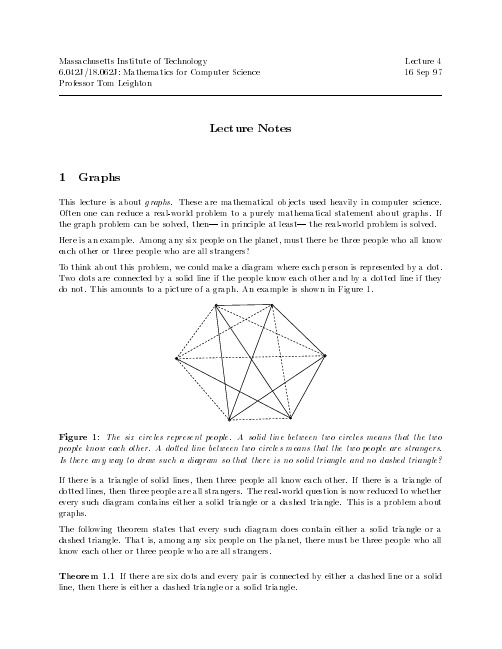
A graph is a pair of sets (V E ). The elements of V are called vertices. The elements of E are called edges. Each edge is a pair of distinct vertices. Graphs are also sometimes called networks. Vertices are also sometimes called nodes. Edges are sometimes called arcs. Graphs can be nicely represented with a diagram of dots and lines as shown in Figure 2 As noted in the de nition, each edge (u v ) 2 E is a pair of distinct vertices u v 2 V . Edge (u v ) is said to be incident to vertices u and v . Vertices u and v are said to be adjacent or neighbors. Phrases like, \an edge joins u and v " and \the edge between u and v " are comon. A computer network is can be modeled nicely as a graph. In this instance, the set of vertices V represents the set of computers in the network. There is an edge (u v) if there is a direct communication link between the computers corresponding to u and v .
高数英文版课件

4 2
3 2 3 2
5(1) 3(1)
42((5252))3522
1 0
0 1
A1A 132
252
4 2
5 3
(3214)4(252)22
(3215)5(252)33
1 0
0 1
Determinant of a Matrix
• The quantity ad – bc that appears in the rule for calculating the inverse of a 2 x 2 matrix is called the determinant of the matrix.
• Here, we investigate division of matrices.
– With this operation, we can solve equations that involve matrices.
• The Inverse of a Matrix
Identity Matrices
b d
Matrices - Operations
When the original matrix is square, transposition does not affect the elements of the main diagonal
Aac
b d
AT
a b
c d
The identity matrix, I, a diagonal matrix D, and a scalar matrix, K, are equal to their transpose since the diagonal is unaffected.
Lectures on Integer Matrices Thomas J. Laffey Contents ...

(with obvious modifications if det A = 0 or if some columns turn out to be zero as the process is implemented). [The process works for nonsquare matrices also]. Multiplying by diag( ±1, . . . , ±1, ±1) if necessary we can ensure that all the diagonal entries are nonnegative. If the element xii is not zero, using further row operations we can replace all the elements xij (j < i) by their remainders on division by xii . In this way we finally obtain a matrix H = (hij ) where the leading entry zi in each nonzero row is positive and the other entries on the corresponding column are nonnegative and less than zi . There exists a matrix U with integer entries such that U A = H and det U = ±1. Both U and H are determined uniquely if det A = 0. H is called the Hermite normal form of A. Examples 3 0 1 3 , 1 1. 2
- 1、下载文档前请自行甄别文档内容的完整性,平台不提供额外的编辑、内容补充、找答案等附加服务。
- 2、"仅部分预览"的文档,不可在线预览部分如存在完整性等问题,可反馈申请退款(可完整预览的文档不适用该条件!)。
- 3、如文档侵犯您的权益,请联系客服反馈,我们会尽快为您处理(人工客服工作时间:9:00-18:30)。
we conclude: • eigenvalues λ1, . . . , λn of −C −1/2GC −1/2 (hence, −C −1G) are real • eigenvectors qi (in xi coordinates) can be chosen orthogonal • eigenvectors in voltage coordinates, si = C −1/2qi, satisfy −C −1Gsi = λisi, sT i Csi = δij
15–6
proof (case of λi distinct) suppose v1, . . . , vn is a set of linearly independent eigenvectors of A: Avi = λivi, then we have
T T T vi (Avj ) = λj vi vj = (Avi)T vj = λivi vj T vj = 0 so (λi − λj )vi T vj = 0 for i = j , λi = λj , hence vi
Symmetric matrices, quadratic forms, matrix norm, and SVD 15–10
Examples
• Bx •
2
= xT B T Bx − xi)2
2
n−1 i=1 (xi+1 2
• Fx
− Gx
sets ms: • { x | f (x) = a } is called a quadratic surface • { x | f (x) ≤ a } is called a quadratic region
Symmetric matrices, quadratic forms, matrix norm, and SVD 15–4
or, geometrically, • rotate by QT • diagonal real scale (‘dilation’) by Λ • rotate back by Q
i=1 n
|vi|2
but also v T Av = (Av ) v = (λv ) v = λ
T T
n i=1
|vi|2
so we have λ = λ, i.e., λ ∈ R (hence, can assume v ∈ Rn)
Symmetric matrices, quadratic forms, matrix norm, and SVD 15–2
Symmetric matrices, quadratic forms, matrix norm, and SVD 15–8
use state xi =
√
civi, so x ˙ = C 1/2v ˙ = −C −1/2GC −1/2x
where C
1/2
√ √ = diag( c1, . . . , cn)
Symmetric matrices, quadratic forms, matrix norm, and SVD 15–14
0)
• A ≥ 0 if and only if λmin(A) ≥ 0, i.e., all eigenvalues are nonnegative
Matrix inequalities
decomposition A=
n T λi q i q i i=1
expresses A as linear combination of 1-dimensional projections
Symmetric matrices, quadratic forms, matrix norm, and SVD
Symmetric matrices, quadratic forms, matrix norm, and SVD 15–7
Example: RC circuit
i1 v1 c1 resistive circuit
in vn cn
ck v ˙ k = −ik ,
i = Gv
G = GT ∈ Rn×n is conductance matrix of resistive circuit thus v ˙ = −C −1Gv where C = diag(c1, . . . , cn) note −C −1G is not symmetric
Symmetric matrices, quadratic forms, matrix norm, and SVD 15–15
many properties that you’d guess hold actually do, e.g., • if A ≥ B and C ≥ D, then A + C ≥ B + D • if B ≤ 0 then A + B ≤ A • if A ≥ 0 and α ≥ 0, then αA ≥ 0 • if A > 0, then A−1 > 0 • A2 ≥ 0
EE263 Autumn 2007-08
Stephen Boyd
Lecture 15 Symmetric matrices, quadratic forms, matrix norm, and SVD
• eigenvectors of symmetric matrices • quadratic forms • inequalities for quadratic forms • positive semidefinite matrices • norm of a matrix • singular value decomposition
replacements A = QΛQT x
Interpretations
QT
QT x
Λ
ΛQT x
Q
Ax
linear mapping y = Ax can be decomposed as • resolve into qi coordinates • scale coordinates by λi • reconstitute with basis qi
hence we can express A as
n
A = QΛQT =
i=1
T λi q i q i
in particular, qi are both left and right eigenvectors
Symmetric matrices, quadratic forms, matrix norm, and SVD 15–3
• we say A is negative semidefinite if −A ≥ 0 • we say A is negative definite if −A > 0 • otherwise, we say A is indefinite matrix inequality: if B = B T ∈ Rn we say A ≥ B if A − B ≥ 0, A < B if B − A > 0, etc. for example: • A ≥ 0 means A is positive semidefinite • A > B means xT Ax > xT Bx for all x = 0
15–1
Eigenvalues of symmetric matrices
suppose A ∈ Rn×n is symmetric, i.e., A = AT fact: the eigenvalues of A are real to see this, suppose Av = λv , v = 0, v ∈ Cn then v T Av = v T (Av ) = λv T v = λ
xT Ax = xT QΛQT x = (QT x)T Λ(QT x)
n
=
i=1
T x)2 λi(qi n
≤ λ1
T x)2 (qi i=1 2
= λ1 x i.e., we have xT Ax ≤ λ1xT x
Symmetric matrices, quadratic forms, matrix norm, and SVD
so the inequalities are tight
Symmetric matrices, quadratic forms, matrix norm, and SVD
15–13
Positive semidefinite and positive definite matrices
suppose A = AT ∈ Rn×n we say A is positive semidefinite if xT Ax ≥ 0 for all x • denoted A ≥ 0 (and sometimes A • not the same as Aij ≥ 0 for all i, j we say A is positive definite if xT Ax > 0 for all x = 0 • denoted A > 0 • A > 0 if and only if λmin(A) > 0, i.e., all eigenvalues are positive
vi = 1
• in this case we can say: eigenvectors are orthogonal • in general case (λi not distinct) we must say: eigenvectors can be chosen to be orthogonal
Eigenvectors of symmetric matrices
fact: there is a set of orthonormal eigenvectors of A, i.e., q1, . . . , qn s.t. T qj = δij Aqi = λiqi, qi in matrix form: there is an orthogonal Q s.t. Q−1AQ = QT AQ = Λ