MATLAB编程作业
完整版优化设计Matlab编程作业
化设计hl4HU©0⑥ 3 hlu 凹内r d X1州fci-rU-fFF卢F ♦ 忡下¥为+1 —*— S-ll-« F41:Si —MATLABoftiHMirjirCfiffliiiiJ PHI■1**■ 温不平?」11,・—喜M - 〜FT 文词一时y 片 34ml 3F*L9TR0i. Jill!-LkftLgWf 1S1CSI掰f 1 ■ >A A A »W I % :k Dnfl w I ■ J k^lXMprfaMk tjn nn Alflhw初选 x0=[1,1] 程序:Step 1: Write an Mfle objfunl.m.function f1=objfun1(x)f1=x(1)人2+2*x(2)入2-2*x(1)*x(2)-4*x(1);Step 2: Invoke one of the unconstrained optimization routinesx0=[1,1];>> options = 0Ptimset('LargeScale','off);>> [x,fval,exitflag,output] = fminunc(@objfun1,x0,options)运行结果: x =4.0000 2.0000 fval = -8.0000exitflag =1 output = iterations: 3 funcCount: 12 stepsize: 1 firstorderopt: 2.3842e-007algorithm: 'medium-scale: Quasi-Newton line search message: [1x85 char]非线性有约束优化1. Min f(x)=3 x : + x 2+2 x 1-3 x 2+5 Subject to:g 2(x)=5 X 1-3 X 2 -25 < 0 g (x)=13 X -41 X 2 < 0 3 12g 4(x)=14 < X 1 < 130无约束优化 min f(x)=X 2 + x 2-2 x 1 x 2-4 x 1g5 (x)=2 < X 2 < 57初选x0=[10,10]Step 1: Write an M-file objfun2.mfunction f2=objfun2(x)f2=3*x(1)人2+x(2)人2+2*x(1)-3*x(2)+5;Step 2: Write an M-file confunl.m for the constraints. function [c,ceq]=confun1(x) % Nonlinear inequality constraints c=[x(1)+x(2)+18;5*x(1)-3*x(2)-25;13*x(1)-41*x(2)人2;14-x(1);x(1)-130;2-x(2);x(2)-57];% Nonlinear inequality constraints ceq=[];Step 3: Invoke constrained optimization routinex0=[10,10]; % Make a starting guess at the solution>> options = optimset('LargeScale','off);>> [x, fval]=...fmincon(@objfun2,x0,[],[],[],[],[],[],@confun1,options)运行结果:x =3.6755 -7.0744 fval =124.14952.min f (x) =4x2 + 5x2s.t. g 1(x) = 2X] + 3x2- 6 < 0g (x) = x x +1 > 0初选x0=[1,1]Step 1: Write an M-file objfun3.m function f=objfun3(x) f=4*x(1)人2 + 5*x(2)人2Step 2: Write an M-file confun3.m for the constraints. function [c,ceq]=confun3(x) %Nonlinear inequality constraints c=[2*x(1)+3*x(2)-6;-x(1)*x(2)-1];% Nonlinear equality constraints ceq口;Step 3: Invoke constrained optimization routinex0=[1,1];% Make a starting guess at the solution>> options = optimset('LargeScale','off);>> [x, fval]=...fmincon(@objfun,x0,[],[],[],[],[],[],@confun,options)运行结果:Optimization terminated: no feasible solution found. Magnitude of search direction less than2*options.TolX but constraints are not satisfied.x =11fval =-13实例:螺栓连接的优化设计图示为一压气机气缸与缸盖连接的示意图。
MATLAB编程练习(含答案很好的)
001双峰曲线图:z=peaks(40);mesh(z);surf(z)002解方程:A=[3,4,-2;6,2,-3;45,5,4];>> B=[14;4;23];>> root=inv(A)*B003傅里叶变换load mtlb ;subplot(2,1,1);plot(mtlb);>> title('原始语音信息');>> y=fft(mtlb);>> subplot(2,1,2);>> yy=abs(y);>> plot(yy);>> title('傅里叶变换')004输入函数:a=input('How many apples\n','s')005输出函数a=[1 2 3 4 ;5 6 7 8;12 23 34 45;34 435 23 34]a =1 2 3 45 6 7 812 23 34 4534 435 23 34disp(a)a =1 2 3 45 6 7 812 23 34 4534 435 23 34b=input('how many people\n' ,'s')how many peopletwo peopleb =two people>> disp(b)two people>>006求一元二次方程的根a=1;b=2;c=3;d=sqrt(b^2-4*a*c);x1=(-b+d)/(2*a)x1 =-1.0000 + 1.4142i>> x2=(-b-d)/(2*a)x2 =-1.0000 - 1.4142i007求矩阵的相乘、转置、存盘、读入数据A=[1 3 5 ;2 4 6;-1 0 -2;-3 0 0];>> B=[-1 3;-2 2;2 1];>> C=A*BC =3 142 20-3 -53 -9>> C=C'C =3 2 -3 314 20 -5 -9>> save mydat C>> clear>> load mydat C008编写数学计算公式:A=2.1;B=-4.5;C=6;D=3.5;E=-5;K=atan(((2*pi*A)+E/(2*pi*B*C))/D) K =1.3121009A=[1 0 -1;2 4 1;-2 0 5];>> B=[0 -1 0;2 1 3;1 1 2];>> H=2*A+BH =2 -1 -26 9 5-3 1 12>> M=A^2-3*BM =3 3 -62 13 -2-15 -3 21>> Y=A*BY =-1 -2 -29 3 145 7 10>> R=B*AR =-2 -4 -1-2 4 14-1 4 10>> E=A.*BE =0 0 04 4 3-2 0 10>> W=A\BW =0.3333 -1.3333 0.66670.2500 1.0000 0.25000.3333 -0.3333 0.6667 >> P=A/BP =-2.0000 3.0000 -5.0000-5.0000 3.0000 -4.00007.0000 -9.0000 16.0000>> Z=A.\BWarning: Divide by zero.Z =0 -Inf 01.0000 0.2500 3.0000-0.5000 Inf 0.4000>> D=A./BWarning: Divide by zero.D =Inf 0 -Inf1.0000 4.0000 0.3333-2.0000 0 2.5000010a=4.96;b=8.11;>> M=exp(a+b)/log10(a+b)M =4.2507e+005011求三角形面积:a=9.6;b=13.7;c=19.4;>> s=(a+b+c)/2;>> area=sqrt(s*(s-a)*(s-b)*(s-c))area =61.1739012逻辑运算A=[-1 0 -6 8;-9 4 0 12.3;0 0 -5.1 -2;0 -23 0 -7]; >> B=A(:,1:2)B =-1 0-9 40 00 -23>> C=A(1:2,:)C =-1.0000 0 -6.0000 8.0000 -9.0000 4.0000 0 12.3000>> D=B'D =-1 -9 0 00 4 0 -23>> A*Bans =1.0000 -184.0000-27.0000 -266.90000 46.0000 207.0000 69.0000>> C<Dans =0 0 1 01 0 0 0>> C&Dans =1 0 0 00 1 0 1>> C|Dans =1 1 1 11 1 0 1>> ~C|~Dans =0 1 1 11 0 1 0013矩阵运算练习:A=[8 9 5;36 -7 11;21 -8 5]A =8 9 536 -7 1121 -8 5>> BB =-1 3 -22 0 3-3 1 9>> RT=A*BRT =-5 29 56-83 119 6-52 68 -21>> QW=A.*BQW =-8 27 -1072 0 33-63 -8 45>> ER=A^3ER =6272 3342 294415714 -856 52608142 -1906 2390 >> BF=A.^3BF =512 729 12546656 -343 13319261 -512 125 >> A/Bans =3.13414.9634 -0.4024-1.2561 12.5244 -3.2317-1.9878 6.4512 -2.0366>> EKV=B\AEKV =10.7195 -1.2683 3.52449.4756 1.5854 3.71954.8537 -1.4878 1.3171>> KDK=[A,B]KDK =8 9 5 -1 3 -236 -7 11 2 0 321 -8 5 -3 1 9 >> ERI=[A;B]ERI =8 9 536 -7 1121 -8 5-1 3 -22 0 3-3 1 9014一般函数的调用:A=[2 34 88 390 848 939];>> S=sum(A)S =2301>> min(A)ans =2>> EE=mean(A)EE =383.5000>> QQ=std(A)QQ =419.3794>> AO=sort(A)AO =2 34 88 390 848 939 >> yr=norm(A)yr =1.3273e+003>> RT=prod(A)RT =1.8583e+012>> gradient(A)ans =32.0000 43.0000 178.0000 380.0000 274.5000 91.0000 >> max(A)ans =939>> median(A)ans =239>> diff(A)ans =32 54 302 458 91>> length(A)ans =6>> sum(A)ans =2301>> cov(A)ans =1.7588e+005>>015矩阵变换:A=[34 44 23;8 34 23;34 55 2]A =34 44 238 34 2334 55 2>> tril(A)ans =34 0 08 34 034 55 2>> triu(A)ans =34 44 230 34 230 0 2>> diag(A)ans =34342norm(A)ans =94.5106>> rank(A)ans =3>> det(A)ans =-23462>> trace(A)ans =70>> null(A)ans =Empty matrix: 3-by-0>> eig(A)ans =80.158712.7671-22.9257>> poly(A)ans =1.0e+004 *0.0001 -0.0070 -0.1107 2.3462>> logm(A)Warning: Principal matrix logarithm is not defined for A with nonpositive real eigenvalues. A non-principal matrixlogarithm is returned.> In funm at 153In logm at 27ans =3.1909 + 0.1314i 1.2707 + 0.1437i 0.5011 - 0.2538i0.4648 + 0.4974i 3.3955 + 0.5438i 0.1504 - 0.9608i0.2935 - 1.2769i 0.8069 - 1.3960i 3.4768 + 2.4663i>> fumn(A)Undefined command/function 'fumn'.>> inv(A)ans =0.0510 -0.0502 -0.0098-0.0326 0.0304 0.02550.0305 0.0159 -0.0343>> cond(A)ans =8.5072>> chol(A)Error using ==> cholMatrix must be positive definite.>> lu(A)ans =34.0000 44.0000 23.00000.2353 23.6471 17.58821.0000 0.4652 -29.1816>> pinv(A)ans =0.0510 -0.0502 -0.0098-0.0326 0.0304 0.02550.0305 0.0159 -0.0343>> svd(A)ans =94.510622.345611.1095>> expm(A)ans =1.0e+034 *2.1897 4.3968 1.93821.31542.6412 1.16431.8782 3.7712 1.6625>> sqrtm(A)ans =5.2379 + 0.2003i 3.4795 + 0.2190i 1.8946 - 0.3869i0.5241 + 0.7581i 5.1429 + 0.8288i 2.0575 - 1.4644i3.0084 - 1.9461i4.7123 - 2.1276i 2.1454 + 3.7589i >>016多项式的计算:A=[34 44 23;8 34 23;34 55 2]A =34 44 238 34 2334 55 2>> P=poly(A)P =1.0e+004 *0.0001 -0.0070 -0.1107 2.3462>> PPA=poly2str(P,'X')PPA =X^3 - 70 X^2 - 1107 X + 23462017多项式的运算:p=[2 6 8 3];w=[32 56 0 2];>> m=conv(p,w)m =64 304 592 548 180 16 6 >> [q,r]=deconv(w,p)q =16r =0 -40 -128 -46>> dp=polyder(w)dp =96 112 0>> [num,den]=polyder(w,p)num =80 512 724 312 -16den =4 24 68 108 100 48 9>> b=polyfit(p,w,4)Warning: Polynomial is not unique; degree >= number of data points. > In polyfit at 74b =-0.6704 9.2037 -32.2593 0 98.1333>> r=roots(p)r =-1.2119 + 1.0652i-1.2119 - 1.0652i-0.5761018求多项式的商和余p=conv([1 0 2],conv([1 4],[1 1]))p =1 5 6 10 8>> q=[1 0 1 1]q =1 0 1 1>> [w,m]=deconv(p,q)w =1 5m =0 0 5 4 3>> cq=w;cr=m;>> disp([cr,poly2str(m,'x')])5 x^2 + 4 x + 3>> disp([cq,poly2str(w,'x')])x + 5019将分式分解a=[1 5 6];b=[1];>> [r,p,k]=residue(b,a)r =-1.00001.0000p =-3.0000-2.0000k =[]020计算多项式:a=[1 2 3;4 5 6;7 8 9];>> p=[3 0 2 3];>> q=[2 3];>> x=2;>> r=roots(p)r =0.3911 + 1.0609i0.3911 - 1.0609i-0.7822>> p1=conv(p,q)p1 =6 9 4 12 9>> p2=poly(a)p2 =1.0000 -15.0000 -18.0000 -0.0000 >> p3=polyder(p)p3 =9 0 2>> p4=polyval(p,x)p4 =31021求除式和余项:[q,r]=deconv(conv([1 0 2],[1 4]),[1 1 1])022字符串的书写格式:s='student's =student>> name='mary';>> s1=[name s]s1 =marystudent>> s3=[name blanks(3);s]s3 =marystudent>>023交换两个数:clearclca=[1 2 3 4 5];b=[6 7 8 9 10];c=a;a=b;b=c;ab24If语句n=input('enter a number,n=');if n<10nend025 if 双分支结构a=input('enter a number ,a=');b=input('enter a number ,b=');if a>bmax=a;elsemax=b;endmax026三个数按照由大到小的顺序排列:A=15;B=24;C=45;if A<BT=A;A=B;B=T;elseif A<CT=A;A=C;C=T;elseif B<CT=B;B=C;C=T;endABC027建立一个收费优惠系统:price=input('please jinput the price : price=') switch fix(price/100)case[0,1]rate =0;case[2,3,4]rate =3/100;case num2cell(5:9)rate=5/100;case num2cell(10:24)rate=8/100;case num2cell(25:49)rate=10/100;otherwiserate=14/100;endprice=price*(1-rate)028:while循环语句i=0;s=0;while i<=1212s=s+i;i=i+1;ends029,用for循环体语句:sum=0;for i=1:1.5:100;sum=sum+i;endsum030循环的嵌套s=0;for i=1:1:6;for j=1:1:8;s=s+i^j;end;end;s031continue 语句的使用:for i=100:120;if rem(i,7)~=0;continue;end;iend032x=input ('输入X的值x=')if x<1y=x^2;elseif x>1&x<2y=x^2-1;elsey=x^2-2*x+1;endy033求阶乘的累加和sum=0;temp=1;for n=1:10;temp=temp*n;sum=sum+temp;endsum034对角线元素之和sum=0;a=[1 2 3 4;5 6 7 8;9 10 11 12;13 14 15 16]; for i=1:4;sum=sum+a(i,i);endsum035用拟合点绘图A=[12 15.3 16 18 25];B=[50 80 118 125 150.8];plot(A,B)036绘制正玄曲线:x=0:0.05:4*pi;y=sin(x);plot(x,y)037绘制向量x=[1 2 3 4 5 6;7 8 9 10 11 12;13 14 15 16 17 18] plot(x)x=[0 0.2 0.5 0.7 0.6 0.7 1.2 1.5 1.6 1.9 2.3]plot(x)x=0:0.2:2*piy=sin(x)plot(x,y,'m:p')038在正弦函数上加标注:t=0:0.05:2*pi;plot(t,sin(t))set(gca,'xtick',[0 1.4 3.14 56.28])xlabel('t(deg)')ylabel('magnitude(v)')title('this is a example ()\rightarrow 2\pi')text(3.14,sin(3.14),'\leftarrow this zero for\pi')039添加线条标注x=0:0.2:12;plot(x,sin(x),'-',x,1.5*cos(x),':');legend('First','Second',1)040使用hold on 函数x=0:0.2:12;plot(x,sin(x),'-');hold onplot(x,1.5*cos(x),':');041一界面多幅图x=0:0.05:7;y1=sin(x);y2=1.5*cos(x);y3=sin(2*x);y4=5*cos(2*x);subplot(221);plot(x,y1);title('sin(x)')subplot(222);plot(x,y2);title('cos(x)')subplot(223);plot(x,y3);title('sin(2x)')subplot(224);plot(x,y4);title('cos(2x)')042染色效果图x=0:0.05:7;y1=sin(x);y2=1.5*cos(x);y3=sin(2*x);y4=5*cos(2*x);subplot(221);plot(x,y1);title('sin(x)');fill(x,y1,'r') subplot(222);plot(x,y2);title('cos(x)');fill(x,y2,'b') subplot(223);plot(x,y3);title('sin(2x)');fill(x,y3,'k') subplot(224);plot(x,y4);title('cos(2x)');fill(x,y4,'g')043特殊坐标图clcy=[0,0.55,2.5,6.1,8.5,12.1,14.6,17,20,22,22.1] subplot(221);plot(y);title('线性坐标图');subplot(222);semilogx(y);title('x轴对数坐标图');subplot(223);semilogx(y);title('y轴对数坐标图');subplot(224);loglog(y);title('双对数坐标图')t=0:0.01:2*pi;r=2*cos(2*(t-pi/8));polar(t,r)044特殊函数绘图:fplot('cos(tan(pi*x))',[-0.4,1.4])fplot('sin(exp(pi*x))',[-0.4,1.4])045饼形图与条形图:x=[8 20 36 24 12];subplot(221);pie(x,[1 0 0 0 1]);title('饼图');subplot(222);bar(x,'group');title('垂直条形图');subplot(223);bar(x,'stack');title('累加值为纵坐标的垂直条形图'); subplot(224);barh(x,'group');title('水平条形图');046梯形图与正弦函数x=0:0.1:10;y=sin(x);subplot(121);stairs(x);subplot(122);stairs(x,y);047概率图x=randn(1,1000);y=-2:0.1:2;hist(x,y)048向量图:x=[-2+3j,3+4j,1-7j];subplot(121);compass(x);rea=[-2 3 1];imag=[3 4 -7];subplot(122);feather(rea,imag);049绘制三维曲线图:z=0:pi/50:10*pi;x=sin(z);y=cos(z);plot3(x,y,z)x=-10:0.5:10;y=-8:0.5:8;[x,y]=meshgrid(x,y);z=sin(sqrt(x.^2+y.^2))./sqrt(x.^2+y.^2); subplot(221);mesh(x,y,z);title('普通一维网格曲面');subplot(222);meshc(x,y,z);title('带等高线的三维网格曲面'); subplot(223);meshz(x,y,z);title('带底座的三维网格曲面'); subplot(224);surf(x,y,z);title('充填颜色的三维网格面')050 带网格二维图x=0:pi/10:2*pi;y1=sin(x);y2=cos(x);plot(x,y1,'r+-',x,y2,'k*:')grid onxlabel('Independent Variable x') ylabel('Dependent Variable y1&y2') text(1.5,0.5,'cos(x)')051各种统计图y=[18 5 28 17;24 12 36 14;15 6 30 9]; subplot(221);bar(y)x=[4,6,8];subplot(222);bar3(x,y)subplot(223);bar(x,y,'grouped') subplot(224);bar(x,y,'stack')052曲面图x=-2:0.4:2;y=-1:0.2:1;[x,y]=meshgrid(x,y);z=sqrt(4-x.^2/9-y.^2/4); surf(x,y,z)grid on053创建符号矩阵e=[1 3 5;2 4 6;7 9 11];m=sym(e)符号表达式的计算问题因式分解:syms xf=factor(x^3-1)s=sym('sin(a+b)'); expand(s)syms x tf=x*(x*(x-8)+6)*t; collect(f)syms xf=sin(x)^2+cos(x)^2; simplify(f)syms xs=(4*x^2+8*x+3)/(2*x+1); simplify(s)通分syms x yf=x/y-y/x;[m,n]=numden(f)嵌套重写syms xf=x^4+3*x^3-7*x^2+12; horner(f)054求极限syms x a;limit(exp(-x),x,0,'left')求导数syms xdiff(x^9+x^6)diff(x^9+x^6,4)055求不定积分与定积分syms x ys=(4-3*x^2)^2;int(s)int(x/(x+y),x)int(x^2/(x+2),x,1,3) double(ans)056函数的变换:syms x ty=exp(-x^2);Ft=fourier(y,x,t)fx=ifourier(Ft,t,x)057求解方程syms a b c xs=a*x^2+b*x+c;solve(s)syms x y zs1=2*x^2+y^2-3*z-4;s2=y+z-3;s3=x-2*y-3*z;[x,y,z]=solve(s1,s2,s3)058求微分方程:y=dsolve('Dy-(t^2+y^2)/t^2/2','t')059求级数和syms x ksymsum(k)symsum(k^2-3,0,10)symsum(x^k/k,k,1,inf)060泰勒展开式syms xs=(1-x+x^2)/(1+x+x^2);taylor(s)taylor(s,9)taylor(s,x,12)taylor(s,x,12,5)061练习syms x a;s1=sin(2*x)/sin(5*x);limit(s1,x,0)s2=(1+1/x)^(2*x);limit(s2,x,inf)syms xs=x*cos(x);diff(s)diff(s,2)diff(s,12)syms xs1=x^4/(1+x^2);int(s1)s2=3*x^2-x+1int(s2,0,2)syms x y zs1=5*x+6*y+7*z-16;s2=4*x-5*y+z-7;s3=x+y+2*z-2;[x,y,z]=solve(s1,s2,s3)syms x yy=dsolve('Dy=exp(2*x-y)','x')y=dsolve('Dy=exp(2*x-y)','y(0)=0','x')n=sym('n');s=symsum(1/n^2,n,1,inf)x=sym('x');f=sqrt(1-2*x+x^3)-(1-3*x+x^2)^(1/3);taylor(f,6)062求于矩阵相关的值a=[2 2 -1 1;4 3 -1 2;8 5 -3 4;3 3 -2 2]adet=det(a)atrace=trace(a)anorm=norm(a)acond=cond(a)arank=rank(a)eiga=eig(a)063矩阵计算A=[0.1389 0.6038 0.0153 0.9318;0.2028 0.2772 0.7468 0.4660;0.1987 0.1988 0.4451 0.4186]B=var(A)C=std(A)D=range(A)E=cov(A)F=corrcoef(A)064求根及求代数式的值P=[4 -3 2 5];x=roots(P)x=[3 3.6];F=polyval(P,x)065多项式的和差积商运算:f=[1 2 -4 3 -1]g=[1 0 1]g1=[0 0 1 0 1]f+g1f-g1conv(f,g)[q,r]=deconv(f,g)polyder(f)066各种插值运算:X=0:0.1:pi/2;Y=sin(X);interp1(X,Y,pi/4)interp1(X,Y,pi/4,'nearest')interp1(X,Y,pi/4,'spline')interp1(X,Y,pi/4,'cubic')067曲线的拟合:X=0:0.1:2*pi;Y=cos(X);[p,s]=polyfit(X,Y,4)plot(X,Y,'K*',X,polyval(p,X),'r-')068求函数的最值与0点x=2:0.1:2;[x,y]=fminbnd('x.^3-2*x+1',-1,1) [x,y]=fzero('x.^3-2*x+1',1)069求多项式的表达式、值、及图像y=[1 3 5 7 19]t=poly(y)x=-4:0.5:8yx=polyval(t,x)plot(x,yx)070数据的拟合与绘图x=0:0.1:2*pi;y=sin(x);p=polyfit(x,y,5);y1=polyval(p,x)plot(x,y,'b',x,y1,'r')071求代数式的极限:syms xf=sym('log(1+2*x)/sin(3*x)');b=limit(f,x,0)072求导数与微分syms xf=sym('x/(cos(x))^2');y1=diff(f)y2=int(f,0,1)078划分网格函数[x,y]=meshgrid(-2:0.01:2,-3:0.01:5); t=x.*exp(-x.^2-y.^2);[px,py]=gradient(t,0.05,0.1);td=sqrt(px.^2+py.^2);subplot(221)imagesc(t)subplot(222)imagesc(td)colormap('gray')079求多次多项方程组的解:syms x1 x2 a ;eq1=sym('x1^2+x2=a')eq2=sym('x1-a*x2=0')[x1 x2]=solve(eq1,eq2,x1,x2)v=solve(eq1,eq2)v.x1v.x2an1=x1(1),an2=x1(2)an3=x2(1),an4=x2(2)080求解微分方程:[y]=dsolve('Dy=-y^2+6*y','y(0)=1','x')s=dsolve('Dy=-y^2+6*y','y(0)=1','x')[u]=dsolve('Du=-u^2+6*u','u(0)=1')w=dsolve('Du=-u^2+6*u','z')[u,w]=dsolve('Du=-w^2+6*w,Dw=sin(z)','u(0)=1,w(0)=0','z') v=dsolve('Du=-w^2+6*w,Dw=sin(z)','u(0)=1,w(0)=0','z')081各种显现隐含函数绘图:f=sym('x^2+1')subplot(221)ezplot(f,[-2,2])subplot(222)ezplot('y^2-x^6-1',[-2,2],[0,10])x=sym('cos(t)')y=sym('sin(t)')subplot(223)ezplot(x,y)z=sym('t^2')subplot(224)ezplot3(x,y,z,[0,8*pi])082极坐标图:r=sym('4*sin(3*x)')ezpolar(r,[0,6*pi])083多函数在一个坐标系内:x=0:0.1:8;y1=sin(x);subplot(221)plot(x,y1)subplot(222)plot(x,y1,x,y2)w=[2 3;3 1;4 6]subplot(223)plot(w)q=[4 6:3 5:1 2]subplot(224)plot(w,q)084调整刻度图像:x=0:0.1:10;y1=sin(x);y2=exp(x);y3=exp(x).*sin(x);subplot(221)plot(x,y2)subplot(222)loglog(x,y2)subplot(223)plotyy(x,y1,x,y2)085等高线等图形,三维图:t=0:pi/50:10*pi;subplot(2,3,1)plot3(t.*sin(t),t.*cos(t),t.^2) grid on[x,y]=meshgrid([-2:0.1:2])z=x.*exp(-x.^2-y.^2)subplot(2,3,2)plot3(x,y,z)box offsubplot(2,3,3)meshz(x,y,z)subplot(2,3,4)surf(x,y,z)contour(x,y,z)subplot(2,3,6)surf(x,y,z)subplot(2,3,5)contour(x,y,z)box offsubplot(2,3,6)contour3(x,y,z)axis off086统计图Y=[5 2 1;8 7 3;9 8 6;5 5 5;4 3 2]subplot(221)bar(Y)box offsubplot(222)bar3(Y)subplot(223)barh(Y)subplot(224)bar3h(Y)087面积图Y=[5 1 2;8 3 7;9 6 8;5 5 5;4 2 3];subplot(221)area(Y)grid onset(gca,'Layer','top','XTick',1:5)sales=[51.6 82.4 90.8 59.1 47.0];x=90:94;profits=[19.3 34.2 61.4 50.5 29.4];subplot(222)area(x,sales,'facecolor',[0.5 0.9 0.6], 'edgecolor','b','linewidth',2) hold onarea(x,profits,'facecolor',[0.9 0.85 0.7], 'edgecolor','y','linewidth',2) hold offset(gca,'Xtick',[90:94])set(gca,'layer','top')gtext('\leftarrow 销售量') gtext('利润')gtext('费用')xlabel('年','fontsize',14)088函数的插值:x=0:2*pi;y=sin(x);xi=0:0.1:8;yi1=interp1(x,y,xi,'linear')yi2=interp1(x,y,xi,'nearest') yi3=interp1(x,y,xi,'spline')yi4=interp1(x,y,xi,'cublic')p=polyfit(x,y,3)yy=polyval(p,xi)subplot(3,2,1)plot(x,y,'o')subplot(3,2,2)plot(x,y,'o',xi,yy)subplot(3,2,3)plot(x,y,'o',xi,yi1)subplot(3,2,4)plot(x,y,'o',xi,yi2)subplot(3,2,5)plot(x,y,'o',xi,yi3)subplot(3,2,6)plot(x,y,'o',xi,yi4)089二维插值计算:[x,y]=meshgrid(-3:0.5:3);z=peaks(x,y);[xi,yi]=meshgrid(-3:0.1:3); zi=interp2(x,y,z,xi,yi,'spline') plot3(x,y,z)hold onmesh(xi,yi,zi+15)hold offaxis tight090函数表达式;function f=exlin(x)if x<0f=-1;elseif x<1f=x;elseif x<2f=2-x;elsef=0;end091:硬循环语句:n=5;for i=1:nfor j=1:nif i==ja(i,j)=2;elsea(i,j)=0;endendendwhile 循环语句:n=1;while prod(1:n)<99^99;n=n+1endn:092 switch开关语句a=input('a=?')switch acase 1disp('It is raning') case 0disp('It do not know')case -1disp('It is not ranging')otherwisedisp('It is raning ?')end093画曲面函数:x1=linspace(-3,3,30)y1=linspace(-3,13,34)[x,y]=meshgrid(x1,y1);z=x.^4+3*x.^2-2*x+6-2*y.*x.^2+y.^2-2*y; surf(x,y,z)。
matlb课程设计作业

matlb课程设计作业一、教学目标本课程的教学目标是使学生掌握MATLAB基本语法、编程技巧以及应用方法,培养学生解决实际问题的能力。
具体目标如下:1.知识目标:(1)理解MATLAB的基本概念,如变量、数据类型、运算符等。
(2)掌握MATLAB编程的基本语法,如矩阵操作、函数定义与调用、循环结构、条件语句等。
(3)熟悉MATLAB与其他软件(如Mathematica、Python等)的接口转换。
(4)了解MATLAB在工程领域中的应用,如信号处理、控制系统、图像处理等。
2.技能目标:(1)能够运用MATLAB进行简单的数学计算、数据分析及图形绘制。
(2)具备编写MATLAB脚本文件和函数文件的能力。
(3)学会使用MATLAB解决实际问题,如编写程序实现线性方程组求解、最优化问题求解等。
(4)掌握MATLAB在实验数据处理、仿真实验等方面的应用。
3.情感态度价值观目标:(1)培养学生对科学探究的兴趣,提高其创新意识。
(2)培养学生团队协作、沟通交流的能力。
(3)培养学生具备良好的编程习惯和职业道德。
二、教学内容本课程的教学内容主要包括以下几个部分:1.MATLAB基本概念:变量、数据类型、运算符等。
2.MATLAB编程语法:矩阵操作、函数定义与调用、循环结构、条件语句等。
3.MATLAB高级应用:数组运算、图像处理、控制系统、信号处理等。
4.MATLAB与其他软件的接口转换。
5.实践项目:利用MATLAB解决实际问题,如线性方程组求解、最优化问题求解等。
三、教学方法本课程采用讲授法、案例分析法、实验法等多种教学方法相结合,以提高学生的学习兴趣和主动性。
1.讲授法:用于讲解MATLAB基本概念、语法和应用。
2.案例分析法:通过分析实际案例,使学生掌握MATLAB在各个领域的应用。
3.实验法:让学生亲自动手实践,培养其运用MATLAB解决实际问题的能力。
四、教学资源1.教材:选用《MATLAB教程》作为主要教材,辅助以相关参考书籍。
matlab编程实例100例
1-32是:图形应用篇33-66是:界面设计篇67-84是:图形处理篇85-100是:数值分析篇实例1:三角函数曲线(1)function shili01h0=figure('toolbar','none',...'position',[198 56 350 300],...'name','实例01');h1=axes('parent',h0,...'visible','off');x=-pi:0.05:pi;y=sin(x);plot(x,y);xlabel('自变量X');ylabel('函数值Y');title('SIN( )函数曲线');grid on实例2:三角函数曲线(2)function shili02h0=figure('toolbar','none',...'position',[200 150 450 350],...'name','实例02');x=-pi:0.05:pi;y=sin(x)+cos(x);plot(x,y,'-*r','linewidth',1);grid onxlabel('自变量X');ylabel('函数值Y');title('三角函数');实例3:图形的叠加function shili03h0=figure('toolbar','none',...'position',[200 150 450 350],...'name','实例03');x=-pi:0.05:pi;y1=sin(x);y2=cos(x);plot(x,y1,...'-*r',...x,y2,...'--og');grid onxlabel('自变量X');ylabel('函数值Y');title('三角函数');实例4:双y轴图形的绘制function shili04h0=figure('toolbar','none',...'position',[200 150 450 250],...'name','实例04');x=0:900;a=1000;b=0.005;y1=2*x;y2=cos(b*x);[haxes,hline1,hline2]=plotyy(x,y1,x,y2,'semilogy','plot'); axes(haxes(1))ylabel('semilog plot');axes(haxes(2))ylabel('linear plot');实例5:单个轴窗口显示多个图形function shili05h0=figure('toolbar','none',...'position',[200 150 450 250],...'name','实例05');t=0:pi/10:2*pi;[x,y]=meshgrid(t);subplot(2,2,1)plot(sin(t),cos(t))axis equalsubplot(2,2,2)z=sin(x)-cos(y);plot(t,z)axis([0 2*pi -2 2])subplot(2,2,3)h=sin(x)+cos(y);plot(t,h)axis([0 2*pi -2 2])subplot(2,2,4)g=(sin(x).^2)-(cos(y).^2);plot(t,g)axis([0 2*pi -1 1])实例6:图形标注function shili06h0=figure('toolbar','none',...'position',[200 150 450 400],...'name','实例06');t=0:pi/10:2*pi;h=plot(t,sin(t));xlabel('t=0到2\pi','fontsize',16);ylabel('sin(t)','fontsize',16);title('\it{从0to2\pi 的正弦曲线}','fontsize',16) x=get(h,'xdata');y=get(h,'ydata');imin=find(min(y)==y);imax=find(max(y)==y);text(x(imin),y(imin),...['\leftarrow最小值=',num2str(y(imin))],...'fontsize',16)text(x(imax),y(imax),...['\leftarrow最大值=',num2str(y(imax))],...'fontsize',16)实例7:条形图形function shili07h0=figure('toolbar','none',...'position',[200 150 450 350],...'name','实例07');tiao1=[562 548 224 545 41 445 745 512];tiao2=[47 48 57 58 54 52 65 48];t=0:7;bar(t,tiao1)xlabel('X轴');ylabel('TIAO1值');h1=gca;h2=axes('position',get(h1,'position'));plot(t,tiao2,'linewidth',3)set(h2,'yaxislocation','right','color','none','xticklabel',[]) 实例8:区域图形function shili08h0=figure('toolbar','none',...'position',[200 150 450 250],...'name','实例08');x=91:95;profits1=[88 75 84 93 77];profits2=[51 64 54 56 68];profits3=[42 54 34 25 24];profits4=[26 38 18 15 4];area(x,profits1,'facecolor',[0.5 0.9 0.6],...'edgecolor','b',...'linewidth',3)hold onarea(x,profits2,'facecolor',[0.9 0.85 0.7],...'edgecolor','y',...'linewidth',3)hold onarea(x,profits3,'facecolor',[0.3 0.6 0.7],...'edgecolor','r',...'linewidth',3)hold onarea(x,profits4,'facecolor',[0.6 0.5 0.9],...'edgecolor','m',...'linewidth',3)hold offset(gca,'xtick',[91:95])set(gca,'layer','top')gtext('\leftarrow第一季度销量')gtext('\leftarrow第二季度销量')gtext('\leftarrow第三季度销量')gtext('\leftarrow第四季度销量')xlabel('年','fontsize',16);ylabel('销售量','fontsize',16);实例9:饼图的绘制function shili09h0=figure('toolbar','none',...'position',[200 150 450 250],...'name','实例09');t=[54 21 35;68 54 35;45 25 12;48 68 45;68 54 69];x=sum(t);h=pie(x);textobjs=findobj(h,'type','text');str1=get(textobjs,{'string'});val1=get(textobjs,{'extent'});oldext=cat(1,val1{:});names={'商品一:';'商品二:';'商品三:'};str2=strcat(names,str1);set(textobjs,{'string'},str2)val2=get(textobjs,{'extent'});newext=cat(1,val2{:});offset=sign(oldext(:,1)).*(newext(:,3)-oldext(:,3))/2; pos=get(textobjs,{'position'});textpos=cat(1,pos{:});textpos(:,1)=textpos(:,1)+offset;set(textobjs,{'position'},num2cell(textpos,[3,2]))实例10:阶梯图function shili10h0=figure('toolbar','none',...'position',[200 150 450 400],...'name','实例10');a=0.01;b=0.5;t=0:10;f=exp(-a*t).*sin(b*t);stairs(t,f)hold onplot(t,f,':*')hold offglabel='函数e^{-(\alpha*t)}sin\beta*t的阶梯图'; gtext(glabel,'fontsize',16)xlabel('t=0:10','fontsize',16)axis([0 10 -1.2 1.2])实例11:枝干图function shili11h0=figure('toolbar','none',...'position',[200 150 450 350],...'name','实例11');x=0:pi/20:2*pi;y1=sin(x);y2=cos(x);h1=stem(x,y1+y2);hold onh2=plot(x,y1,'^r',x,y2,'*g');hold offh3=[h1(1);h2];legend(h3,'y1+y2','y1=sin(x)','y2=cos(x)') xlabel('自变量X');ylabel('函数值Y');title('正弦函数与余弦函数的线性组合');实例12:罗盘图function shili12h0=figure('toolbar','none',...'position',[200 150 450 250],...'name','实例12');winddirection=[54 24 65 84256 12 235 62125 324 34 254];windpower=[2 5 5 36 8 12 76 14 10 8];rdirection=winddirection*pi/180;[x,y]=pol2cart(rdirection,windpower); compass(x,y);desc={'风向和风力','气象台','10月1日0:00到','10月1日12:00'};gtext(desc)实例13:轮廓图function shili13h0=figure('toolbar','none',...'position',[200 150 450 250],...'name','实例13');[th,r]=meshgrid((0:10:360)*pi/180,0:0.05:1); [x,y]=pol2cart(th,r);z=x+i*y;f=(z.^4-1).^(0.25);contour(x,y,abs(f),20)axis equalxlabel('实部','fontsize',16);ylabel('虚部','fontsize',16);h=polar([0 2*pi],[0 1]);delete(h)hold oncontour(x,y,abs(f),20)实例14:交互式图形function shili14h0=figure('toolbar','none',...'position',[200 150 450 250],...'name','实例14');axis([0 10 0 10]);hold onx=[];y=[];n=0;disp('单击鼠标左键点取需要的点'); disp('单击鼠标右键点取最后一个点'); but=1;while but==1[xi,yi,but]=ginput(1);plot(xi,yi,'bo')n=n+1;disp('单击鼠标左键点取下一个点');x(n,1)=xi;y(n,1)=yi;endt=1:n;ts=1:0.1:n;xs=spline(t,x,ts);ys=spline(t,y,ts);plot(xs,ys,'r-');hold off实例14:交互式图形function shili14h0=figure('toolbar','none',...'position',[200 150 450 250],...'name','实例14');axis([0 10 0 10]);hold onx=[];y=[];n=0;disp('单击鼠标左键点取需要的点'); disp('单击鼠标右键点取最后一个点'); but=1;while but==1[xi,yi,but]=ginput(1);plot(xi,yi,'bo')n=n+1;disp('单击鼠标左键点取下一个点');x(n,1)=xi;y(n,1)=yi;endt=1:n;ts=1:0.1:n;xs=spline(t,x,ts);ys=spline(t,y,ts);plot(xs,ys,'r-');hold off实例15:变换的傅立叶函数曲线function shili15h0=figure('toolbar','none',...'position',[200 150 450 250],...'name','实例15');axis equalm=moviein(20,gcf);set(gca,'nextplot','replacechildren') h=uicontrol('style','slider','position',...[100 10 500 20],'min',1,'max',20) for j=1:20plot(fft(eye(j+16)))set(h,'value',j)m(:,j)=getframe(gcf);endclf;axes('position',[0 0 1 1]);movie(m,30)实例16:劳伦兹非线形方程的无序活动function shili15h0=figure('toolbar','none',...'position',[200 150 450 250],...'name','实例15');axis equalm=moviein(20,gcf);set(gca,'nextplot','replacechildren') h=uicontrol('style','slider','position',...[100 10 500 20],'min',1,'max',20) for j=1:20plot(fft(eye(j+16)))set(h,'value',j)m(:,j)=getframe(gcf);endclf;axes('position',[0 0 1 1]);movie(m,30)实例17:填充图function shili17h0=figure('toolbar','none',...'position',[200 150 450 250],...'name','实例17');t=(1:2:15)*pi/8;x=sin(t);y=cos(t);fill(x,y,'r')axis square offtext(0,0,'STOP',...'color',[1 1 1],...'fontsize',50,...'horizontalalignment','center') 例18:条形图和阶梯形图function shili18h0=figure('toolbar','none',...'position',[200 150 450 250],...'name','实例18');subplot(2,2,1)x=-3:0.2:3;y=exp(-x.*x);bar(x,y)title('2-D Bar Chart')subplot(2,2,2)x=-3:0.2:3;y=exp(-x.*x);bar3(x,y,'r')title('3-D Bar Chart')subplot(2,2,3)x=-3:0.2:3;y=exp(-x.*x);stairs(x,y)title('Stair Chart')subplot(2,2,4)x=-3:0.2:3;y=exp(-x.*x);barh(x,y)title('Horizontal Bar Chart')实例19:三维曲线图function shili19h0=figure('toolbar','none',...'position',[200 150 450 400],...'name','实例19');subplot(2,1,1)x=linspace(0,2*pi);y1=sin(x);y2=cos(x);y3=sin(x)+cos(x);z1=zeros(size(x));z2=0.5*z1;z3=z1;plot3(x,y1,z1,x,y2,z2,x,y3,z3)grid onxlabel('X轴');ylabel('Y轴');zlabel('Z轴');title('Figure1:3-D Plot')subplot(2,1,2)x=linspace(0,2*pi);y1=sin(x);y2=cos(x);y3=sin(x)+cos(x);z1=zeros(size(x));z2=0.5*z1;z3=z1;plot3(x,z1,y1,x,z2,y2,x,z3,y3)grid onxlabel('X轴');ylabel('Y轴');zlabel('Z轴');title('Figure2:3-D Plot')实例20:图形的隐藏属性function shili20h0=figure('toolbar','none',...'position',[200 150 450 300],...'name','实例20');subplot(1,2,1)[x,y,z]=sphere(10);mesh(x,y,z)axis offtitle('Figure1:Opaque')hidden onsubplot(1,2,2)[x,y,z]=sphere(10);mesh(x,y,z)axis offtitle('Figure2:Transparent') hidden off实例21PEAKS函数曲线function shili21h0=figure('toolbar','none',...'position',[200 100 450 450],...'name','实例21');[x,y,z]=peaks(30);subplot(2,1,1)x=x(1,:);y=y(:,1);i=find(y>0.8&y<1.2);j=find(x>-0.6&x<0.5);z(i,j)=nan*z(i,j);surfc(x,y,z)xlabel('X轴');ylabel('Y轴');zlabel('Z轴');title('Figure1:surfc函数形成的曲面') subplot(2,1,2)x=x(1,:);y=y(:,1);i=find(y>0.8&y<1.2);j=find(x>-0.6&x<0.5);z(i,j)=nan*z(i,j);surfl(x,y,z)xlabel('X轴');ylabel('Y轴');zlabel('Z轴');title('Figure2:surfl函数形成的曲面')实例22:片状图function shili22h0=figure('toolbar','none',...'position',[200 150 550 350],...'name','实例22');subplot(1,2,1)x=rand(1,20);y=rand(1,20);z=peaks(x,y*pi);t=delaunay(x,y);trimesh(t,x,y,z)hidden offtitle('Figure1:Triangular Surface Plot'); subplot(1,2,2)x=rand(1,20);y=rand(1,20);z=peaks(x,y*pi);t=delaunay(x,y);trisurf(t,x,y,z)title('Figure1:Triangular Surface Plot'); 实例23:视角的调整function shili23h0=figure('toolbar','none',...'position',[200 150 450 350],...'name','实例23');x=-5:0.5:5;[x,y]=meshgrid(x);r=sqrt(x.^2+y.^2)+eps;z=sin(r)./r;subplot(2,2,1)surf(x,y,z)xlabel('X-axis')ylabel('Y-axis')zlabel('Z-axis')title('Figure1')view(-37.5,30)subplot(2,2,2)surf(x,y,z)xlabel('X-axis')ylabel('Y-axis')zlabel('Z-axis')title('Figure2')view(-37.5+90,30)subplot(2,2,3)surf(x,y,z)xlabel('X-axis')ylabel('Y-axis')zlabel('Z-axis')title('Figure3')view(-37.5,60)subplot(2,2,4)surf(x,y,z)xlabel('X-axis')ylabel('Y-axis')zlabel('Z-axis')title('Figure4')view(180,0)实例24:向量场的绘制function shili24h0=figure('toolbar','none',...'position',[200 150 450 350],...'name','实例24');subplot(2,2,1)z=peaks;ribbon(z)title('Figure1')subplot(2,2,2)[x,y,z]=peaks(15);[dx,dy]=gradient(z,0.5,0.5); contour(x,y,z,10)hold onquiver(x,y,dx,dy)hold offtitle('Figure2')subplot(2,2,3)[x,y,z]=peaks(15);[nx,ny,nz]=surfnorm(x,y,z);surf(x,y,z)hold onquiver3(x,y,z,nx,ny,nz)hold offtitle('Figure3')subplot(2,2,4)x=rand(3,5);y=rand(3,5);z=rand(3,5);c=rand(3,5);fill3(x,y,z,c)grid ontitle('Figure4')实例25:灯光定位function shili25h0=figure('toolbar','none',...'position',[200 150 450 250],...'name','实例25');vert=[1 1 1;1 2 1;2 2 1;2 1 1;1 1 2;12 2;2 2 2;2 1 2];fac=[1 2 3 4;2 6 7 3;4 3 7 8;15 8 4;1 2 6 5;5 6 7 8];grid offsphere(36)h=findobj('type','surface');set(h,'facelighting','phong',...'facecolor',...'interp',...'edgecolor',[0.4 0.4 0.4],...'backfacelighting',...'lit')hold onpatch('faces',fac,'vertices',vert,...'facecolor','y');light('position',[1 3 2]);light('position',[-3 -1 3]); material shinyaxis vis3d offhold off实例26:柱状图function shili26h0=figure('toolbar','none',...'position',[200 50 450 450],...'name','实例26');subplot(2,1,1)x=[5 2 18 7 39 8 65 5 54 3 2];bar(x)xlabel('X轴');ylabel('Y轴');title('第一子图');subplot(2,1,2)y=[5 2 18 7 39 8 65 5 54 3 2];barh(y)xlabel('X轴');ylabel('Y轴');title('第二子图');实例27:设置照明方式function shili27h0=figure('toolbar','none',...'position',[200 150 450 350],...'name','实例27');subplot(2,2,1)sphereshading flatcamlight leftcamlight rightlighting flatcolorbaraxis offtitle('Figure1')subplot(2,2,2)sphereshading flatcamlight leftcamlight rightlighting gouraudcolorbaraxis offtitle('Figure2')subplot(2,2,3)sphereshading interpcamlight rightcamlight leftlighting phongcolorbaraxis offtitle('Figure3')subplot(2,2,4)sphereshading flatcamlight leftcamlight rightlighting nonecolorbaraxis offtitle('Figure4')实例28:羽状图function shili28h0=figure('toolbar','none',...'position',[200 150 450 350],...'name','实例28');subplot(2,1,1)alpha=90:-10:0;r=ones(size(alpha));m=alpha*pi/180;n=r*10;[u,v]=pol2cart(m,n);feather(u,v)title('羽状图')axis([0 20 0 10])subplot(2,1,2)t=0:0.5:10;x=0.05+i;y=exp(-x*t);feather(y)title('复数矩阵的羽状图')实例29:立体透视(1)function shili29h0=figure('toolbar','none',...'position',[200 150 450 250],...'name','实例29');[x,y,z]=meshgrid(-2:0.1:2,...-2:0.1:2,...-2:0.1:2);v=x.*exp(-x.^2-y.^2-z.^2);grid onfor i=-2:0.5:2;h1=surf(linspace(-2,2,20),...linspace(-2,2,20),...zeros(20)+i);rotate(h1,[1 -1 1],30)dx=get(h1,'xdata');dy=get(h1,'ydata');dz=get(h1,'zdata');delete(h1)slice(x,y,z,v,[-2 2],2,-2)hold onslice(x,y,z,v,dx,dy,dz)hold offaxis tightview(-5,10)drawnowend实例30:立体透视(2)function shili30h0=figure('toolbar','none',...'position',[200 150 450 250],...'name','实例30');[x,y,z]=meshgrid(-2:0.1:2,...-2:0.1:2,...-2:0.1:2);v=x.*exp(-x.^2-y.^2-z.^2); [dx,dy,dz]=cylinder;slice(x,y,z,v,[-2 2],2,-2)for i=-2:0.2:2h=surface(dx+i,dy,dz);rotate(h,[1 0 0],90)xp=get(h,'xdata');yp=get(h,'ydata');zp=get(h,'zdata');delete(h)hold onhs=slice(x,y,z,v,xp,yp,zp);axis tightxlim([-3 3])view(-10,35)drawnowdelete(hs)hold offend实例31:表面图形function shili31h0=figure('toolbar','none',...'position',[200 150 550 250],...'name','实例31');subplot(1,2,1)x=rand(100,1)*16-8;y=rand(100,1)*16-8;r=sqrt(x.^2+y.^2)+eps;z=sin(r)./r;xlin=linspace(min(x),max(x),33); ylin=linspace(min(y),max(y),33); [X,Y]=meshgrid(xlin,ylin);Z=griddata(x,y,z,X,Y,'cubic'); mesh(X,Y,Z)axis tighthold onplot3(x,y,z,'.','Markersize',20)subplot(1,2,2)k=5;n=2^k-1;theta=pi*(-n:2:n)/n;phi=(pi/2)*(-n:2:n)'/n;X=cos(phi)*cos(theta);Y=cos(phi)*sin(theta);Z=sin(phi)*ones(size(theta));colormap([0 0 0;1 1 1])C=hadamard(2^k);surf(X,Y,Z,C)axis square实例32:沿曲线移动的小球h0=figure('toolbar','none',...'position',[198 56 408 468],...'name','实例32');h1=axes('parent',h0,...'position',[0.15 0.45 0.7 0.5],...'visible','on');t=0:pi/24:4*pi;y=sin(t);plot(t,y,'b')n=length(t);h=line('color',[0 0.5 0.5],...'linestyle','.',...'markersize',25,...'erasemode','xor');k1=uicontrol('parent',h0,...'style','pushbutton',...'position',[80 100 50 30],...'string','开始',...'callback',[...'i=1;',...'k=1;,',...'m=0;,',...'while 1,',...'if k==0,',...'break,',...'end,',...'if k~=0,',...'set(h,''xdata'',t(i),''ydata'',y(i)),',...'drawnow;,',...'i=i+1;,',...'if i>n,',...'m=m+1;,',...'i=1;,',...'end,',...'end,',...'end']);k2=uicontrol('parent',h0,...'style','pushbutton',...'position',[180 100 50 30],...'string','停止',...'callback',[...'k=0;,',...'set(e1,''string'',m),',...'p=get(h,''xdata'');,',...'q=get(h,''ydata'');,',...'set(e2,''string'',p);,',...'set(e3,''string'',q)']); k3=uicontrol('parent',h0,...'style','pushbutton',...'position',[280 100 50 30],...'string','关闭',...'callback','close');e1=uicontrol('parent',h0,...'style','edit',...'position',[60 30 60 20]);t1=uicontrol('parent',h0,...'style','text',...'string','循环次数',...'position',[60 50 60 20]);e2=uicontrol('parent',h0,...'style','edit',...'position',[180 30 50 20]); t2=uicontrol('parent',h0,...'style','text',...'string','终点的X坐标值',...'position',[155 50 100 20]); e3=uicontrol('parent',h0,...'style','edit',...'position',[300 30 50 20]); t3=uicontrol('parent',h0,...'style','text',...'string','终点的Y坐标值',...'position',[275 50 100 20]);实例33:曲线转换按钮h0=figure('toolbar','none',...'position',[200 150 450 250],...'name','实例33');x=0:0.5:2*pi;y=sin(x);h=plot(x,y);grid onhuidiao=[...'if i==1,',...'i=0;,',...'y=cos(x);,',...'delete(h),',...'set(hm,''string'',''正弦函数''),',...'h=plot(x,y);,',...'grid on,',...'else if i==0,',...'i=1;,',...'y=sin(x);,',...'set(hm,''string'',''余弦函数''),',...'delete(h),',...'h=plot(x,y);,',...'grid on,',...'end,',...'end'];hm=uicontrol(gcf,'style','pushbutton',...'string','余弦函数',...'callback',huidiao);i=1;set(hm,'position',[250 20 60 20]);set(gca,'position',[0.2 0.2 0.6 0.6])title('按钮的使用')hold on实例34:栅格控制按钮h0=figure('toolbar','none',...'position',[200 150 450 250],...'name','实例34');x=0:0.5:2*pi;y=sin(x);plot(x,y)huidiao1=[...'set(h_toggle2,''value'',0),',...'grid on,',...];huidiao2=[...'set(h_toggle1,''value'',0),',...'grid off,',...];h_toggle1=uicontrol(gcf,'style','togglebutton',...'string','grid on',...'value',0,...'position',[20 45 50 20],...'callback',huidiao1);h_toggle2=uicontrol(gcf,'style','togglebutton',...'string','grid off',...'value',0,...'position',[20 20 50 20],...'callback',huidiao2);set(gca,'position',[0.2 0.2 0.6 0.6])title('开关按钮的使用')实例35:编辑框的使用h0=figure('toolbar','none',...'position',[200 150 350 250],...'name','实例35');f='Please input the letter';huidiao1=[...'g=upper(f);,',...'set(h2_edit,''string'',g),',...];huidiao2=[...'g=lower(f);,',...'set(h2_edit,''string'',g),',...];h1_edit=uicontrol(gcf,'style','edit',...'position',[100 200 100 50],...'HorizontalAlignment','left',...'string','Please input the letter',...'callback','f=get(h1_edit,''string'');',...'background','w',...'max',5,...'min',1);h2_edit=uicontrol(gcf,'style','edit',...'HorizontalAlignment','left',...'position',[100 100 100 50],...'max',5,...'min',1);h1_button=uicontrol(gcf,'style','pushbutton',...'string','小写变大写',...'position',[100 45 100 20],...'callback',huidiao1);h2_button=uicontrol(gcf,'style','pushbutton',...'string','大写变小写',...'position',[100 20 100 20],...'callback',huidiao2);实例36:弹出式菜单h0=figure('toolbar','none',...'position',[200 150 450 250],...'name','实例36');x=0:0.5:2*pi;y=sin(x);h=plot(x,y);grid onhm=uicontrol(gcf,'style','popupmenu',...'string',...'sin(x)|cos(x)|sin(x)+cos(x)|exp(-sin(x))',...'position',[250 20 50 20]);set(hm,'value',1)huidiao=[...'v=get(hm,''value'');,',...'switch v,',...'case 1,',...'delete(h),',...'y=sin(x);,',...'h=plot(x,y);,',...'grid on,',...'case 2,',...'delete(h),',...'y=cos(x);,',...'h=plot(x,y);,',...'grid on,',...'case 3,',...'delete(h),',...'y=sin(x)+cos(x);,',...'h=plot(x,y);,',...'grid on,',...'case 4,',...'y=exp(-sin(x));,',...'h=plot(x,y);,',...'grid on,',...'end'];set(hm,'callback',huidiao)set(gca,'position',[0.2 0.2 0.6 0.6])title('弹出式菜单的使用')实例37:滑标的使用h0=figure('toolbar','none',...'position',[200 150 450 250],...'name','实例37');[x,y]=meshgrid(-8:0.5:8);r=sqrt(x.^2+y.^2)+eps;z=sin(r)./r;h0=mesh(x,y,z);h1=axes('position',...[0.2 0.2 0.5 0.5],...'visible','off');htext=uicontrol(gcf,...'units','points',...'position',[20 30 45 15],...'string','brightness',...'style','text');hslider=uicontrol(gcf,...'units','points',...'position',[10 10 300 15],...'min',-1,...'max',1,...'style','slider',...'callback',...'brighten(get(hslider,''value''))');实例38:多选菜单h0=figure('toolbar','none',...'position',[200 150 450 250],...'name','实例38');[x,y]=meshgrid(-8:0.5:8);r=sqrt(x.^2+y.^2)+eps;z=sin(r)./r;h0=mesh(x,y,z);hlist=uicontrol(gcf,'style','listbox',...'string','default|spring|summer|autumn|winter',...'max',5,...'min',1,...'position',[20 20 80 100],...'callback',[...'k=get(hlist,''value'');,',...'switch k,',...'case 1,',...'colormap default,',...'case 2,',...'colormap spring,',...'case 3,',...'colormap summer,',...'case 4,',...'colormap autumn,',...'case 5,',...'colormap winter,',...'end']);实例39:菜单控制的使用h0=figure('toolbar','none',...'position',[200 150 450 250],...'name','实例39');x=0:0.5:2*pi;y=cos(x);h=plot(x,y);grid onset(gcf,'toolbar','none')hm=uimenu('label','example');huidiao1=[...'set(hm_gridon,''checked'',''on''),',...'set(hm_gridoff,''checked'',''off''),',...'grid on'];huidiao2=[...'set(hm_gridoff,''checked'',''on''),',...'set(hm_gridon,''checked'',''off''),',...'grid off'];hm_gridon=uimenu(hm,'label','grid on',...'checked','on',...'callback',huidiao1);hm_gridoff=uimenu(hm,'label','grid off',...'checked','off',...'callback',huidiao2);实例40:UIMENU菜单的应用。
matlab简单编程21个题目及答案
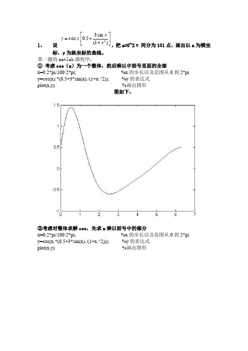
1、设⎥⎦⎤⎢⎣⎡++=)1(sin35.0cos2xxxy,把x=0~2π间分为101点,画出以x为横坐标,y为纵坐标的曲线。
第一题的matlab源程序:①考虑cos(x)为一个整体,然后乘以中括号里面的全部x=0:2*pi/100:2*pi; %x的步长以及范围从0到2*pi y=cos(x).*(0.5+3*sin(x)./(1+x.^2)); %y的表达式plot(x,y)%画出图形图如下:②考虑对整体求解cos,先求x乘以括号中的部分x=0:2*pi/100:2*pi; %x的步长以及范围从0到2*pi y=cos(x.*(0.5+3*sin(x)./(1+x.^2))); %y的表达式plot(x,y) %画出图形图如下:2、产生8×6阶的正态分布随机数矩阵R1, 求其各列的平均值和均方差。
并求该矩阵全体数的平均值和均方差。
第二题的matlab源程序如下:R1=randn(8,6) %产生正态分布随机矩阵R1 =1.0933 -0.7697 1.5442 -0.1924 1.4193 0.21571.1093 0.3714 0.0859 0.8886 0.2916 -1.1658-0.8637 -0.2256 -1.4916 -0.7648 0.1978 -1.14800.0774 1.1174 -0.7423 -1.4023 1.5877 0.1049-1.2141 -1.0891 -1.0616 -1.4224 -0.8045 0.7223-1.1135 0.0326 2.3505 0.4882 0.6966 2.5855-0.0068 0.5525 -0.6156 -0.1774 0.8351 -0.66691.5326 1.1006 0.7481 -0.1961 -0.2437 0.1873aver=(sum(R1(1:end,1:end)))./8 %产生各行的平均值aver =0.0768 0.1363 0.1022 -0.3473 0.4975 0.1044a=std(R1(1:end,1:end)) %产生各行的均方差也就是标准差a =1.0819 0.8093 1.3456 0.8233 0.8079 1.2150aver1=(sum(R1(:)))./48 %全体数的平均值aver1 =0.0950b=std(R1(:)) %全体数的均方差即标准差b =1.01033、设x=rcost+3t,y=rsint+3,分别令r=2,3,4,画出参数t=0~10区间生成的x~y 曲线。
matlab编程题整理

作业一1输出x,y两个中值较大的一个值x=input(‘x’);y=input(‘y’);if x>yxelseyend2输入x,计算y的值。
计算函数的值y=x+1,x<0,y=2x-1,x≧0x=input错误!未指定书签。
(‘x);if x<0y=x+1elsey=2*x-1end3输入一学生成绩,评定其等级,方法是:90~100分为“优秀”,80~89分为“良好”,70~79分为“中等”,60~69分为“及格”,60分为“不合格”x=input(‘x’)if x>100|x<0y=’输入错误’elseif x>=90y=’优秀’elseif x>=80y=’良好’elseif x>=70y=’中等’elseif x>=60y=’及格’elsey=’不合格’emd4某超市节日期间举办购物打折的促销活动,优惠办法是:每位顾客当天一次性购物在100元以上者,按九五折优惠;在200元以上者,按九折优惠;在300元以上者,按八五折优惠;在500元以上者,按八折优惠。
x=input(‘x’);if x>=500y=x*0.8elseif x>=300y=x*0.85elseif x>=200y=x*0.9elseif x>=100y=x*0.95else y=xend 5编程计算:s=1+2+3+…+100sum=0;for i=1:100sum=sum+i;endsum引申1!-2!+3!-4!+5!- (99)sum=0;for i=1:99pdr=1;for k=1:ipdr=pdr*k;endsum=sum+pdr*(-1)^(i-1);endsum引申1*2*3*4*……*100sum=1;for i=1:100sum=sum*iendsum6计算1~100的奇数和sum=0;for i=1:2:100sum=sum+i;endsum7百元买百鸡问题。
计算力学(有限元)matlab编程大作业(空间网架)
M=jiedianlianjie(n);
L=l(M,N,n);
%n*n 的矩阵,用于存储 n 个节点的连接关系,连接则对应元素为 1,否则为 0 %n*n 矩阵,用于存储 I,j 节点连接所得的杆件的长度
Y=ganjiangeshu(L,n); %数量值,表示杆件的个数 t=T(L,N,n); %3n*3n 矩阵,用于存储以上各杆件的坐标转换矩阵 S=dangangjihe(E,A,n,Y,L,t); %6*6y 矩阵,用于存储 y 根杆件的各自的单刚矩阵 K=zonggang(E,A,L,t,n); %3n*3n 矩阵,描述总刚 P=zhiling(K); %总刚矩阵主元根据约束条件置零 Q=jia1(P,n); %总刚矩阵置零主元加 1 z=lixiangliang(n); %由输入力组成的列向量 p=inv(Q)*z; %求解位移 F=neili(n,Y,S,L,p); %由位移及单刚矩阵求得各杆件内力 三、命令执行输入参数及计算结果: (5 节点九单元,实际模型见下图)
五、有限元软件验算 模型建立:
模型计算结果:
软件内力输出: (此处内力是 x,y,z 方向的合力) 1 节点荷载 0.000000 0.000000 2 节点荷载 0.000000 0.000000 3 节点荷载 0.000000 0.000000 4 节点荷载 -325.269119 -325.269119 5 节点荷载 230.000000 230.000000 6 节点荷载 0.000000 0.000000 7 节点荷载 0.000000 0.000000 8 节点荷载 0.000000 0.000000 9 节点荷载 -1732.050808 -1732.050808 软件位移输出: 1 节点荷载 0.000000 0.000000 0.000000 0.000000 0.000000 0.000000 2 节点荷载 0.002273 0.000440 0.000115 0.000000 0.000000 0.000000 3 节点荷载 0.000000 0.000000 0.000000 0.000000 0.000000 0.000000 4 节点荷载 0.000000 0.000000 -0.002158 0.000000 0.000000 0.000000 5 节点荷载 0.000000 0.000000 0.000000 0.000000 0.000000 0.000000 完全一致。 六、窗口命令输入(分段力考虑非线性,在上文窗口命令的基础上输入) a=maxbianxing(L,p,n,Y); %找出所有杆件中(位移/杆长)最大值 [f,nmax]=fenduanli(z,a); %求出单元加载力向量以及需要加载的次数(nmax) [d,G,LL]=feixianxing(E,A,f,Q,N,n,M,P,nmax); %求出考虑非线性下的位移 d,并输出最终变形后的坐
matlab简单编程21个题目及答案
1、设⎥⎦⎤⎢⎣⎡++=)1(sin35.0cos2xxxy,把x=0~2π间分为101点,画出以x为横坐标,y为纵坐标的曲线。
第一题的matlab源程序:①考虑cos(x)为一个整体,然后乘以中括号里面的全部x=0:2*pi/100:2*pi; %x的步长以及范围从0到2*pi y=cos(x).*(0.5+3*sin(x)./(1+x.^2)); %y的表达式plot(x,y)%画出图形图如下:②考虑对整体求解cos,先求x乘以括号中的部分x=0:2*pi/100:2*pi; %x的步长以及范围从0到2*pi y=cos(x.*(0.5+3*sin(x)./(1+x.^2))); %y的表达式plot(x,y) %画出图形图如下:2、产生8×6阶的正态分布随机数矩阵R1, 求其各列的平均值和均方差。
并求该矩阵全体数的平均值和均方差。
第二题的matlab源程序如下:R1=randn(8,6) %产生正态分布随机矩阵R1 =1.0933 -0.7697 1.5442 -0.1924 1.4193 0.21571.1093 0.3714 0.0859 0.8886 0.2916 -1.1658-0.8637 -0.2256 -1.4916 -0.7648 0.1978 -1.14800.0774 1.1174 -0.7423 -1.4023 1.5877 0.1049-1.2141 -1.0891 -1.0616 -1.4224 -0.8045 0.7223-1.1135 0.0326 2.3505 0.4882 0.6966 2.5855-0.0068 0.5525 -0.6156 -0.1774 0.8351 -0.66691.5326 1.1006 0.7481 -0.1961 -0.2437 0.1873aver=(sum(R1(1:end,1:end)))./8 %产生各行的平均值aver =0.0768 0.1363 0.1022 -0.3473 0.4975 0.1044a=std(R1(1:end,1:end)) %产生各行的均方差也就是标准差a =1.0819 0.8093 1.3456 0.8233 0.8079 1.2150aver1=(sum(R1(:)))./48 %全体数的平均值aver1 =0.0950b=std(R1(:)) %全体数的均方差即标准差b =1.01033、设x=rcost+3t,y=rsint+3,分别令r=2,3,4,画出参数t=0~10区间生成的x~y 曲线。
matlab编程经典例题
3.2 程序控制结构 3.2.1 顺序结构 1.数据的输入 从键盘输入数据,则可以使用input函数来进
行,该函数的调用格式为: A=input(提示信息,选项); 其中提示信息为一个字符串,用于提示用户 输入什么样的数据。 如果在input函数调用时采用's'选项,则允 许用户输入一个字符串。例如,想输入一 个人的姓名,可采用命令: xm=input('What''s your name?','s');
%输出商品实际销售价格
3.try语句 语句格式为:
try 语句组1
catch 语句组2
end try语句先试探性执行语句组1,如果语句组1
在执行过程中出现错误,则将错误信息赋 给保留的lasterr变量,并转去执行语句组2。
1
例3-7 矩阵乘法运算要求两矩阵的维数相容,否则 会出错。先求两矩阵的乘积,若出错,则自动转 去求两矩阵的点乘。
语句组m
else 语句组n
end 语句用于实现多分支选择结构。
1
例3-5 输入一个字符,若为大写字母,则输出其 对应的小写字母;若为小写字母,则输出其对应 的大写字母;若为数字字符则输出其对应的数值, 若为其他字符则原样输出。 c=input('请输入一个字符','s'); if c>='A' & c<='Z' disp(setstr(abs(c)+abs('a')-abs('A'))); elseif c>='a'& c<='z' disp(setstr(abs(c)- abs('a')+abs('A'))); elseif c>='0'& c<='9' disp(abs(c)-abs('0')); else disp(c); end
matlab编程例题
matlab编程例题Matlab是一种高级的计算机编程语言和数学计算软件。
它具有强大的数据处理和可视化功能,可以用于各种科学计算、数据分析、模拟和建模等领域。
本文将介绍一些常见的Matlab编程例题,帮助初学者掌握Matlab的基本编程技能。
1. 矩阵运算矩阵是Matlab中最基本的数据类型之一,可以进行各种数学运算。
下面是一些矩阵运算的例子:a = [1 2 3; 4 5 6; 7 8 9]; %定义一个3×3的矩阵b = [10 20 30; 40 50 60; 70 80 90]; %定义另一个3×3的矩阵c = a + b; %矩阵加法d = a - b; %矩阵减法e = a * b; %矩阵乘法f = a' %矩阵转置运行上面的代码,可以得到以下结果:c =11 22 3344 55 6677 88 99d =-9 -18 -27-36 -45 -54-63 -72 -81e =300 360 420660 810 9601020 1260 1500f =1 4 72 5 83 6 92. 绘图Matlab具有强大的绘图功能,可以绘制各种二维和三维图形。
下面是一些绘图的例子:x = linspace(0, 2*pi, 100); %生成一个包含100个点的等间隔向量y = sin(x); %计算sin函数plot(x, y); %绘制sin函数图像z = peaks(25); %生成一个25×25的山峰矩阵surf(z); %绘制3D山峰图像运行上面的代码,可以得到以下结果:sin函数图像:3D山峰图像:3. 文件读写Matlab可以读写各种文件格式,包括文本文件、Excel文件、图像文件等。
下面是一些文件读写的例子:fid = fopen('data.txt', 'r'); %打开名为“data.txt”的文本文件data = fscanf(fid, '%f'); %读取文件中的数据fclose(fid); %关闭文件plot(data); %绘制数据图像A = xlsread('data.xlsx'); %读取名为“data.xlsx”的Excel 文件plot(A(:, 1), A(:, 2)); %绘制Excel文件中的数据图像运行上面的代码,可以得到以下结果:文本文件数据图像:Excel文件数据图像:4. 函数编写Matlab中的函数是一种可重复使用的代码块,可以让程序更加模块化和可读性更高。
- 1、下载文档前请自行甄别文档内容的完整性,平台不提供额外的编辑、内容补充、找答案等附加服务。
- 2、"仅部分预览"的文档,不可在线预览部分如存在完整性等问题,可反馈申请退款(可完整预览的文档不适用该条件!)。
- 3、如文档侵犯您的权益,请联系客服反馈,我们会尽快为您处理(人工客服工作时间:9:00-18:30)。
《Matlab 编程训练》作业专业学生姓名 班级 学号指导教师 完成日期实训一 MATLAB 语言介绍和数值计算1.先求下列表达式的值,然后显示MATLAB 工作空间的使用情况并保存变量。
122sin851z e=+.2. 已知 1234413134787,2033657327A B --⎡⎤⎡⎤⎢⎥⎢⎥==⎢⎥⎢⎥⎢⎥⎢⎥-⎣⎦⎣⎦,求下列表达式的值: (1) A+6*B 和A-B+I (其中I 为单位矩阵)A+6*B:A-B+I:(2)A*B和A.*BA*B程序:A=[12 34 -4;34 7 87;3 65 7]B=[1 3 -1;2 0 3;3 -2 7]c=A*B结果:A.*B程序:A=[12 34 -4;34 7 87;3 65 7]B=[1 3 -1;2 0 3;3 -2 7]D=A.*B结果:(3)A^3和A.^3A^3程序:A=[12 34 -4;34 7 87;3 65 7]E=A^3结果:A.^3程序:A=[12 34 -4;34 7 87;3 65 7]C=A.^3(4)A/B及B\AA/B程序:A=[12 34 -4;34 7 87;3 65 7]B=[1 3 -1;2 0 3;3 -2 7]C=A/B结果:B\A程序:A=[12 34 -4;34 7 87;3 65 7]B=[1 3 -1;2 0 3;3 -2 7]D=B\A结果:(5)将矩阵C=B\A的右下角2*2子矩阵赋给D, 并(3)保存变量(mat文件)程序:A=[12 34 -4;34 7 87;3 65 7];B=[1 3 -1;2 0 3;3 -2 7];C=B*inv(A);D=C(2:3,2:3)结果:3. 求得矩阵⎥⎥⎥⎥⎦⎤⎢⎢⎢⎢⎣⎡=34157864653434533145A 的每行最大元素所在的位置?(至少两种方法) 第一种:A=[5 14 33;45 43 3;65 4 6;78 15 34][RowMax Order]=max(A')结果:第二种:A=[5 14 33;45 43 3;65 4 6;78 15 34][Max_num,index]=max(A,[],2)结果:实训二 MATLAB 编程基础1. 求[25,1258]之间能被15整除的数的个数。
程序: A=25:1258;length(A(mod(A,15)==0)) 结果:2. 根据222221 (3121116)n ++++=π,求π的近似值。
当n 分别取100、1000、10000时,结果是多少?程序:n=1:100;test=sqrt(6*sum(1./(n.*n))) 结果:程序:n=1:1000;test=sqrt(6*sum(1./(n.*n))) 结果:程序:n=1:10000;test=sqrt(6*sum(1./(n.*n)))结果:3. 有三个多项式p1(x)=x4+2x3+4x2+5,p2(x)=x+2,p3(x)=x2+2x+3,试进行下列操作:(1)求P(x)=P1(x)+P2(x)P3(x);程序:p2=[1 2]p3=[1 2 3]Q=conv(p2,p3)结果:程序:p1=[1 2 4 0 5]Q1=[0 1 4 7 6]B=p1+Q1结果:(2)求P(x)的根;程序:C=roots(B)结果:(3)当x 取矩阵A 的每一元素时,求P(x)的值,其中⎥⎥⎥⎦⎤⎢⎢⎢⎣⎡--=5.2505.3275.04.12.11A 程序:A=[-1 1.2 -1.4;0.75 2 3.5;0 5 2.5] y=polyval(B,A)结果:(4)当以矩阵A 为自变量时,求P(x)的值,其中A 的值与(3)题相同。
程序:A=[-1 1.2 -1.4;0.75 2 3.5;0 5 2.5] y1=polyvalm(B,A)结果:实训三 MATLAB 图形系统1. 设x xxy sin ]5cos 101.0[3++=,在x =0~2π区间取120点,绘制函数曲线。
程序:x=(0:2*pi/119:2*pi)y=(0.1+10*cos(x)/(5+x.^3))*sin(x); plot(x,y) 结果:2. 已知y1=x 2,y2=cos(2x),y3=y1*y2,完成下列操作(x ∈(0,10)):(1)在同一坐标系下用不同的颜色和线型绘制三条曲线;(2)在不同的图形窗中分别用条形图、阶梯图、杆图绘制三条曲线。
如下图所示:3. 微分方程求解:2332121121,),(bx x x x x x f x m x a x-=+-=+-= 其中,.7/2,7/1,28.14,910=-===m m b a )11)((2/11101--+-=x x m m f ,初始值]0.2 0.30.2[0=x .实训四 SIMULINK 仿真环境1. 利用SIMULINK 仿真来实现摄氏温度到华氏温度的转化:3259c f +=T T (c T 范围在-10℃~100℃)2. 单位负反馈系统的开环传递函数为:)101.0)(11.0(1000)(++=s s s s G ,应用Simulink 仿真系统构建阶跃响应曲线。
3. 分析PID 调节器各参数的作用PID 的数学模型为01()()(()())tp DIde t u t K e t e t T T dt=++⎰1)、分析PID调节作用,考查当(1)Kp=8.5,Ki=5.3,Kd=3.4 (2)Kp=6.7,Ki=2,Kd=2.5 (3)Kp=4.2,Ki=1.8,Kd=1.7 时对系统阶跃响应的影响. (三条线在一个图里)2)、以Kp=8.5,Ki=5.3,Kd=3.4这组数据为基础,改变其中一个参数,固定其余两个,以此来分别讨论Kp,Ki,Kd的作用(三条线在一个图里):①分析PID的比例作用: 只改变Kp,当Kp=8.5, Kp=6.7, Kp=4.2时候系统输出曲线截图标注;②分析PID的积分作用:只改变Ki,当Ki=5.3, Ki=2, Ki=1.8时候系统输出曲线截图标注;③分析PID的微分作用:只改变Kd,当Kd=3.4, Kd=2.5, Kd=1.7时候系统输出曲线截图标注。
3)、分析不同调节器下该系统的阶跃响应曲线(四条线在一个图里) (1)P调节 Kp=8(2)PI调节 Kp=5,Ki=2(3)PD调节 Kp=8.5,Kd=2.5(4)PID调节 Kp=7.5,Ki=5,Kd=3实训五 综合题1. 某控制系统的被控过程的传递函数是:)110)(12)(15(1)(+++=s s s s G ,基于Matlab Simulink 设计PID 控制器,满足以下要求: (PID 控制器封装子系统,写出具体步骤,并附图.) (1)封装子系统(2)设置参数(3)整定PID参数(稳定边界法采用4:1)?设置初始参数为Kp =1,Ki =0,Kd =0(即纯比例控制),启动仿真,得到系统的阶跃响应曲线,如图(a)所示。
由图(a)可知,系统虽然能够稳定运行,但却是有静差的,而且快速性也较差,因此需要引入积分和微分环节。
根据临界比例度法的整定法则,需要逐步增大Kp,获取系统的等幅振荡曲线,求出临界增益Ku 和临界振荡周期Tu。
通过调整参数求得临界振荡时的临界增益为Ku ≈12.5 ,临界振荡周期大致为Tu ≈15.12 s图(a)(4)整定PID参数(稳定边界法采用等幅振荡)?控制器类型Kp Ki KdP 0.5Ku ∞0PI 0.455Ku 0.85Tu 0PID 0.6Ku 0.5Tu 0.125Tu根据表一选取相应的PID参数值应为:Kp=0.6Ku=7.5,Ti=0.5Tu=7.56,Td=0.125,Tu=1.89所以积分项系数Ki=Kp/Ti=0.992,微分项系数为Kd=Kp*Td=14.175。
最后求得按照临界比例度法整定 PID 参数后系统的阶跃响应曲线如图(b)所示。
由图(b)知,系统阶跃响应的超调量,调节时间约为 35s,稳定性和快速性还有待改善,此时可以对整定的 PID 参数适当调整。
通过减小积分系数 Ki 来减小超调量。
取 Ki=0.4,Kp,Kd 仍用临界比例度法整定的数据,进而得到系统新的单位阶跃响应曲线,如图(c)所示。
从图(c)可以看出系统的过渡过程时间,超调量都有所降低。
图(b)图(c)3) 结果分析比较?使用稳态边界法得到的相应曲线调节可以消除余差,但是它的超调量较大。
我们可以把Ki适当减少,即增大积分时间常数,减弱积分作用来改善响应曲线过渡过程动态偏差过大的问题。
2.已知两子系统传递函数分别为:15)(1+=s s G 9287)(22+++=s s s s G 试求:1) 两系统并联连接的等效传递函数,观察其单位阶跃响应;2)两系统串联连接的等效传递函数,观察其单位阶跃响应;3)以G2(s)为前向通道函数,以G1(s)为反馈通道函数,观察其单位阶跃响应。
(要求:分别采用编程和simulink两种方法完成)(1)simulink法:(2)编程法:个人总结为期一个星期的MATLAB实训已经结束,虽然时间很短,但我还是从中学到了很多,对MATLAB有了一定的了解。
Matlab是一个基于矩阵运算的软件,它的运算功能非常强大,编程效率高,强大而智能化的作业图功能,可扩展性强,simulink动态仿真功能,主要用于仿真、验证、算法思想是否正确。
在这段时间里,我们主要学习MATLAB的工具的使用,熟悉其最基础的功能,锻炼了我的实际动手能力。
Help是MATLAB中最有效的命令。
遇到问题,通常都可以借助help解决问题。
就对matlab相关的命令操作而言,通过这次实验的亲身操作和实践,学习掌握了许多原本不知道的或者不太熟悉的命令。
比如说相关m文件的建立,画图用到的标注,配色,坐标控制,同一张图里画几幅不同的图像,相关参数的设置以最后我再次也希望通过这篇总结来表达自己对知道老师的感谢之情,谢谢您的不懈努力和耐心指导,才使得我再这次的实验过程中收获的这么多,也正式您的不吝教诲才使得我们在这次实验中学习和收获了许多的有用的知识和技巧,我相信在以后的学习或者工作中一定有其用武之地。