butterworth filter
巴特沃斯滤波器求阶数n
巴特沃斯滤波器求阶数n
【最新版】
目录
一、巴特沃斯滤波器概述
二、巴特沃斯滤波器的阶数选择
三、巴特沃斯滤波器的设计方法
四、应用实例与结论
正文
一、巴特沃斯滤波器概述
巴特沃斯滤波器(Butterworth filter)是一种常用的数字滤波器,以英国数学家巴特沃斯(Butterworth)的名字命名。
其特点是通频带的频率响应曲线最平滑,能够有效地抑制噪声和杂波,广泛应用于信号处理、通信系统等领域。
二、巴特沃斯滤波器的阶数选择
在设计巴特沃斯滤波器时,一个重要的参数是滤波器的阶数 n。
阶数n 决定了滤波器的性能,如通带截止频率、阻带衰减等。
一般来说,阶数n 越大,滤波器的性能越理想,但同时计算复杂度和成本也会增加。
因此,需要在满足性能要求的前提下,选择合适的阶数 n。
三、巴特沃斯滤波器的设计方法
巴特沃斯滤波器的设计方法通常采用拉普拉斯变换或模拟滤波器原
型法。
拉普拉斯变换是一种数学工具,可以将数字滤波器设计问题转化为一个关于 s(复变量)的方程,然后通过求解该方程得到滤波器的传递函数。
而模拟滤波器原型法则是通过构建一个模拟滤波器,然后根据模拟滤波器的特性设计数字滤波器。
四、应用实例与结论
巴特沃斯滤波器在信号处理和通信系统中有广泛的应用。
例如,在音频处理中,可以使用巴特沃斯滤波器对音频信号进行降噪和音质改善;在通信系统中,可以使用巴特沃斯滤波器对信号进行预处理,以提高信号的可靠性和抗干扰性。
总之,巴特沃斯滤波器是一种优秀的数字滤波器,具有良好的性能和实用性。
butterworth滤波器参数
butterworth滤波器参数Butterworth滤波器是一种常用的模拟滤波器,可用于数字信号处理和图像处理等领域。
在不同的应用场景中,选取不同的Butterworth滤波器参数是非常关键和重要的。
因此,本文将围绕Butterworth滤波器参数展开详细的讲解。
1. Butterworth滤波器简介Butterworth滤波器是一种典型的模拟滤波器,它采用同一阶数下的所有极点具有相等的间隔角度,这使得该滤波器的幅频响应更加均匀。
它的传递函数可以表达为:H(s) = 1 / (1 + (s/ωc)^2n)^0.5其中,s为复频域变量,ωc为截止频率,n为阶数。
2. Butterworth滤波器参数(1) 截止频率(ωc)Butterworth滤波器的截止频率是非常关键的参数,它用于控制Butterworth滤波器截止频率的位置和允许传递带和阻止带的宽度。
截止频率和阶数和直接相关的因素,因为随着阶数的增加,截止频率也会相应地增加。
(2) 阶数 (n)Butterworth滤波器的阶数是指滤波器的极点数量,它决定了滤波器在频率域中的滤波能力。
但同时,随着阶数的增加,滤波器对干扰信号的抑制能力也会增强,但滤波器的相应时间也会变得更慢。
(3) 通带波纹通带波纹是指定义在滤波器通带内的最大允许幅度误差,这个值可以用dB(dB)或百分数(%)来表示。
幅频响应的平滑程度随着通带波纹的增加而降低。
在各种滤波器类型中,Butterworth滤波器的通带波纹最小。
3. Butterworth滤波器参数选择在实际问题中,根据实际应用需要,需要选取不同的Butterworth滤波器参数。
在选择阶数时,应为其提供一个平衡点,在得到足够的滤波效果的同时,保持良好的时间性能。
而正确选择截止频率需要考虑信号的带宽和噪声降低的要求。
需要注意的是,但是在合理范围内将阶数和截止频率的值增加会导致滤波器消失时间过长,从而降低系统的响应速度。
Butter 函数
Butter 函数Butter函数是一个用于设计巴特沃斯滤波器(Butterworth Filter)的函数。
巴特沃斯滤波器是一种常见的数字滤波器,广泛应用于信号处理和数据分析领域。
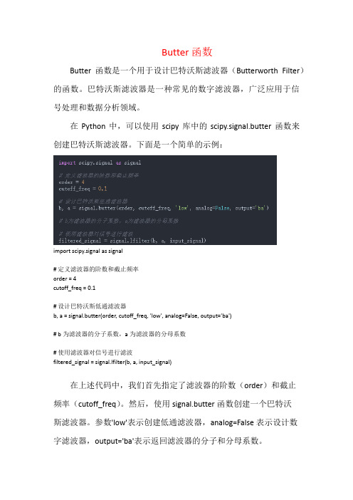
在Python中,可以使用scipy库中的scipy.signal.butter函数来创建巴特沃斯滤波器。
下面是一个简单的示例:import scipy.signal as signal# 定义滤波器的阶数和截止频率order = 4cutoff_freq = 0.1# 设计巴特沃斯低通滤波器b, a = signal.butter(order, cutoff_freq, 'low', analog=False, output='ba')# b为滤波器的分子系数,a为滤波器的分母系数# 使用滤波器对信号进行滤波filtered_signal = signal.lfilter(b, a, input_signal)在上述代码中,我们首先指定了滤波器的阶数(order)和截止频率(cutoff_freq)。
然后,使用signal.butter函数创建一个巴特沃斯滤波器。
参数'low'表示创建低通滤波器,analog=False表示设计数字滤波器,output='ba'表示返回滤波器的分子和分母系数。
创建好滤波器后,我们可以使用signal.lfilter函数将输入信号(input_signal)进行滤波,得到滤波后的信号(filtered_signal)。
当然,根据具体的需求,也可以创建其他类型的巴特沃斯滤波器,如高通、带通或带阻滤波器,只需相应地更改参数'low'为'high'、'bandpass'或'bandstop'即可。
一阶数字滤波器算法
一阶数字滤波器算法
一阶数字滤波器算法常用的有巴特沃斯滤波器、一阶滑动平均滤波器和一阶指数加权滤波器。
以下是这几种滤波器的算法描述:
1. 巴特沃斯滤波器(Butterworth Filter):
巴特沃斯滤波器是一种常用的无纹波滤波器,其算法如下:
- 设输入信号为x,输出信号为y,滤波器的阶数为n,截止频率为fc。
- 初始化y为0。
- 对于每个输入样本xi,进行以下操作:
- 计算y = (1 / (1 + (xi / fc)^2n)) * (y + xi)。
2. 一阶滑动平均滤波器(First-order Moving Average Filter):
一阶滑动平均滤波器是一种简单的滤波器,其算法如下:
- 设输入信号为x,输出信号为y,滤波器的滑动窗口大小为N。
- 初始化y为0。
- 对于每个输入样本xi,进行以下操作:
- 将xi加入到窗口中,并将最旧的样本移除。
- 计算y = (1 / N) * (y * N - oldest_sample + xi)。
3. 一阶指数加权滤波器(First-order Exponential Weighted Filter):
一阶指数加权滤波器是一种常用的滤波器,其算法如下:
- 设输入信号为x,输出信号为y,滤波器的平滑因子为alpha (范围为0到1)。
- 初始化y为0。
- 对于每个输入样本xi,进行以下操作:
- 计算y = alpha * xi + (1 - alpha) * y。
这些算法适用于数字滤波器的实现,具体使用哪种滤波器,取决于应用的要求和滤波器的特性。
巴特沃兹滤波器 (butterworth)
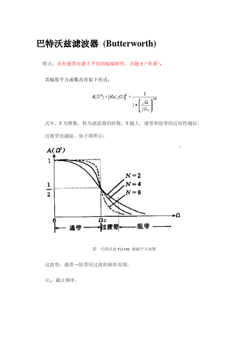
巴特沃兹滤波器(Butterworth)特点:具有通带内最大平坦的振幅特性,且随f↗单调↘其幅度平方函数具有如下形式:式中,N为整数,称为滤波器的阶数,N越大,通带和阻带的近似性越好,过渡带也越陡。
如下图所示:图巴特沃兹filter 振幅平方函数过渡带:通带→阻带间过渡的频率范围,:截止频率。
Ωc理想滤波器的过渡带为O,阻带|H(jΩ)|=0,通带内幅度|H(jΩ)|=常数,H (jΩ)线性相位。
通带内,分母Ω/Ωc<1,相应( Ω/Ωc)2N随N的增加而趋于0,A(Ω2)→1,在过渡带和阻带,Ω/Ωc>1,随N的增加,Ωe/Ωc>>1,所以A(Ω2)快速下降。
Ω=Ωc时,,幅度衰减,相当于3bd衰减点。
振幅平方函数的极点可写成:Ha(-s).Ha(s)=可分解为2N个一次因式令分母为零,→可见,Butterworth 滤波器的振幅平方函数有2N个极点,它们均匀对称地的圆周上。
分布在|s|=Ωc例:如图为N=3阶Butterworth 滤波器振幅平方函数的极点分布。
图三阶A(-s2)的极点分布考虑到系统的稳定性, Butterworth 滤波器的系统函数是由s平面左半部分的极点(SP3,SP4,SP5)组成的,它们分别为:所以系统函数为:式中是为使S=0时Ha(s)=1而引入的。
如用归一化s,即s’=s/Ωc,得归一化的三阶BF:如果要还原的话,则有关于数字滤波器滤波器有很多种,讨论下对信号频率具有选择性的滤波器。
这又分为模拟滤波器和数字滤波器。
模拟滤波器是在传统模拟电路中发展起来的,其实就是RC电路网络。
随着数字技术的发展,数字滤波器则越来越受到青睐。
数字滤波器分为递归型和非递归型,所谓递归即滤波器内部存在反馈回路,这种滤波器对单位冲击响应可以延续到无限长的时间,所以也叫IIR (infinite impulse response filter) ;相应的,非递归型即内部不存在反馈,也叫FIR(finite impulse response filter),其传递函数不存在除零点意外的极点。
Butterworth模拟低通滤波器设计
例:利用AF-BW filter及脉冲响应不变法设计一DF,满足
Wp=0.2p, Ws=0.6p, Ap2dB, As15dB 。
%determine the DF filter [numd,dend]=impinvar(numa,dena,Fs); %plot the frequency response w=linspace(0,pi,1024); h=freqz(numd,dend,w); norm=max(abs(h)); numd=numd/norm; plot(w/pi,20*log10(abs(h/norm))); xlabel('Normalized frequency'); ylabel('Gain,dB'); %computer Ap As of the designed filter w=[Wp Ws]; h=freqz(numd,dend,w); fprintf('Ap= %.4f\n',-20*log10( abs(h(1)))); fprintf('As= %.4f\n',-20*log10( abs(h(2))));
Ap=1.00dB, As=40dB
模拟高通滤波器的设计
MATLAB实现 [numt,dent] = lp2hp(num,den,W0)
例: 设计满足下列条件的模拟BW型高通滤波器 fp=5kHz, fs=1kHz, Ap1dB, As 40dB。
%高通滤波器的设计 wp=1/(2*pi*5000);ws=1/(2*pi*1000);Ap=1;As=40; [N,Wc]=buttord(wp,ws,Ap,As,'s'); [num,den] = butter(N,Wc,'s'); disp('LP 分子多项式'); fprintf('%.4e\n',num); disp('LP 分母多项式'); fprintf('%.4e\n',den); [numt,dent] = lp2hp(num,den,1); disp('HP 分子多项式'); fprintf('%.4e\n',numt); disp('HP 分母多项式'); fprintf(‘%.4e\n’,dent);
Butterworth模拟低通滤波器设计
例:设计满足下列条件的模拟Butterworth低通滤波器
fp=1kHz, fs=2kHz, Ap=1dB, As=40dB
0
BW型: N=8
-20
Gain in dB
-40
-60
-80
0
500
1000
1500
2000
2500
3000
Frequency in Hz
Ap=0.62dB, As=40dB
例:设计满足下列条件的模拟CB I型低通滤波器 fp=1kHz, fs=2kHz, Ap=1dB, As=40dB
%filter specification Wp=2*pi*1000;Ws=2*pi*2000;Ap=1;As=40; %Computer filter order [N,Wc]=cheb1ord(Wp,Ws,Ap,As,'s'); fprintf('Order of the filter=%.0f\n',N) %compute filter coefficients [num,den] = cheby1(N,Ap,Wc,'s'); disp('Numerator polynomial'); fprintf('%.4e\n',num); disp('Denominator polynomial'); fprintf('%.4e\n',den);
Butterworth模拟低通滤波器设计
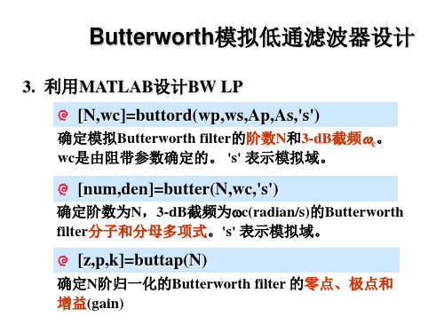
3. 利用MATLAB设计BW LP
[N,wc]=buttord(wp,ws,Ap,As,'s')
确定模拟Butterworth filter的阶数N和3-dB截频wc。
常见的滤波器函数
附件9-2-1 常见的滤波器函数由于理想滤波器的特性不可能实现,因而在实际滤波器的设计中通常采用某个函数来逼近。
根据逼近函数有很多种,以下介绍根据常用的逼近函数所设计的巴特沃兹滤波器(Butterworth filter )、切比雪夫滤波器(Chebyshev filter )和椭圆函数滤波器(elliptic filter )。
由这些函数所决定的实际滤波器特性各有其突出特点,有的衰减特性在过渡区很陡峭,有的相位特性(即延时特性)较为规律,应用中要根据实际需要来选用。
一、巴特沃兹滤波器巴特沃兹滤波器的特点是通带内的频率响应曲线最大限度平坦,没有起伏,而在阻带则逐渐下降为零。
巴特沃兹滤波器的时域特性也比较好,其脉冲响应具有适当的过冲及振铃。
R p =3dB 的巴特沃兹滤波器幅频特性的数学表达式为:()nn f f H 22c 1lg 101lg 10lg 20Ω+-=⎥⎥⎦⎤⎢⎢⎣⎡⎪⎪⎭⎫ ⎝⎛+-=式中f c 是截止频率,Ω=f /f c 是归一化频率,n 是其阶数。
这个响应在Ω=0处有20lg|H |=0dB ,其后随Ω增大而单调增大,在Ω<1即f <f c 的通带内,曲线增长极其缓慢,比较平稳;在Ω>1即f >f c 的阻带内,曲线增长甚快,比较陡峭。
因为函数Ω2n 在Ω=0处的一阶、二阶直至2n -1阶导数均为0,反映了函数的变化率极小,所以巴特沃兹响应也称为最平坦响应。
阻带曲线增长的速率由n 来决定,n 越大,增长越快。
一阶巴特沃兹滤波器的衰减率为每倍频6分贝。
二阶巴特沃兹滤波器的衰减率为每倍频12分贝,三阶巴特沃兹滤波器的衰减率为每倍频18分贝,如此类推。
图1所示为一阶至五阶巴特沃兹低通滤波器的幅频特性。
f20lg|H |/dB图1 一阶至五阶巴特沃兹低通滤波器二、切比雪夫滤波器在巴特沃兹滤波器中,幅度响应在通带内是最平坦且没有起伏的,在阻带内是单调下降的,然而衰减速度相对较为缓慢。
butterworth滤波器阶数
butterworth滤波器阶数Butterworth滤波器是一种常见的模拟滤波器,由英国数学家S. Butterworth在20世纪30年代开发。
它可以应用于信号处理中,常常被用来消除不需要的信号成分,使得滤波后的信号更加适合特定的应用。
Butterworth滤波器的阶数是指滤波器所具有的极点和零点的数量。
根据阶数的不同,可以将Butterworth滤波器分为一阶、二阶、三阶、四阶以及更高阶的滤波器,不同阶数的滤波器具有不同的频率特性和幅频响应。
下面我们将对Butterworth滤波器的阶数进行详细的阐述。
一阶Butterworth滤波器:一阶Butterworth滤波器由一个极点和一个零点组成。
它的幅频响应不是完全的理想低通滤波器,但在0dB时有一点峰值。
一阶滤波器有一个非常简单的形式,因此易于设计和实现。
然而,它的滤波效果并不是最好的。
二阶Butterworth滤波器:二阶Butterworth滤波器由两个极点和两个零点组成。
它具有更好的滤波效果和频率特性,同时也更加复杂。
二阶滤波器是一种比较常见的滤波器,它可以用于各种信号处理应用,例如声音处理和图像处理等。
三阶Butterworth滤波器:三阶Butterworth滤波器比二阶滤波器更加复杂,由三个极点和三个零点组成。
它的滤波效果更好,频率特性也更加平缓。
三阶滤波器通常在需要更加精确滤波时使用,例如高分辨率的数码音频处理。
四阶Butterworth滤波器:四阶Butterworth滤波器具有更加平滑的频率特性和更好的滤波效果。
它由四个极点和四个零点组成,是一种比较复杂的滤波器。
四阶滤波器可以用于处理许多需要高精度滤波的应用,例如声音合成和数字信号处理等。
总结:Butterworth滤波器的阶数越高,滤波效果越好,频率特性越平滑。
不同阶数的滤波器适用于不同的应用场合,需要根据具体应用进行选择。
但需要注意的是,随着阶数的增加,滤波器也变得更加复杂,难以设计和实现。
BUTTERWORTHFILTERDESIGN巴特沃斯滤波器的设计
BUTTERWORTH FILTER DESIGN ObjectiveThe main purpose of this project is to learn the procedures for designing Butterworth filters.BackgroundThe Butterworth and Chebyshev filters are high order filter designs which have significantly different characteristics, but both can be realized by using simple first order or biquad stages cascaded together to achieve the desired order, passband response, and cut-off frequency. The Butterworth filter has a maximally flat response, i.e., no passband ripple and a roll-off of -20dB per pole. In the Butterworth scheme the designer is usually optimizing the flatness of the passband response at the expense of roll-off. The Chebyshev filter displays a much steeper roll-off, but the gain in the passband is not constant. The Chebyshev filter is characterized by a significant passband ripple that often can be ignored. The designer in this case is optimizing roll-off at the expense of passband ripple.Both filter types can be implemented using the simple Sallen-Key configuration. The Sallen-Key design (shown in Figure A-1) is a biquadratic or biquad type filter, meaning there are two poles defined by the circuit transfer function(1)where H 0 is the DC gain of the biquad circuit and is a function only of the ratio of the two resistors connected to the negative input of the opamp. The quantity Q is called the quality factor and is a direct measure of the flatness of the passband (in particular, a large value of Q indicates peaking at the edge of the passband.) When C 1 = C 2 = C and R 1 = R 2 =R for the Sallen-Key design, the value of Q depends exclusively on the gain of the op-amp stage and the cut-off frequency depends on R and C, or(2)(3) Notice that the quality factor Q and the DC gain H 0 cannot be independently set in the)(/)()12(/1s H o H s s o o Q ωω=++12f c RC π=13O Q H =−Sallen-Key circuit. Choice of the value of Q depends on the desired characteristics of the filter. In particular the designer must consider both the quality and the stability of the circuit. Calculations with different values of Q demonstrate that for the second order case the flattest response occurs when Q = 0.707, hence the maximally flat response of the Butterworth filter will also be realized when Q = 0.707. In addition the circuit is only stable when H 0 < 3. Higher values will result in poles in the right half-plane and an unstable circuit.The Butterworth filter is an optimal filter with maximally flat response in the passband. The magnitude of the frequency response of this family of filters can be written as(4)where n is the order of the filter and f c is the cutoff frequency . For a single biquad section, i.e., n = 2, the gain for which Q will equal 0.707, and hence yield a Butterworth type response, is found to be 1.586 from equation (2).In the case of a fourth order Butterworth filter (n = 4), the correct response can be achieved by cascading two biquad stages. Each stage must be characterized by a specific value of gain (or Q ) that achieves both a flat response and stability. For a fourth order Butterworth filter, the Q factors of the two stages must be Q = 0.541 and Q = 1.307. From (2) it follows that one stage must have a gain of 1.152 and the other stage a gain of 2.235. As a result the overall DC gain of the fourth-order Butterworth realized with two biquad stages will be equal to the product of the DC gain of the two stages, i.e., 2.575. The gain values required to cascade biquad sections to achieve even-order filters are given in Table A-I. Note that the number of biquad stages needed to realize a filter of order n is n /2.Other types of filters such as high pass, and bandpass filters can be designed the same way, i.e., by cascading the appropriate filter sections to achieve the desired bandpass and roll-off. The high-pass dual to the Sallen-Key low pass filter can be realized by simply exchanging the positions of R and C in the circuit of Figure A-1. Project1. Design a Butterworth lowpass filter with the following specification:Pass Frequency = 10KHzStop Frequency = 20KHzMinimum Attenuation in the stop band = 45 dB2. Design a Butterworth highpass filter with the following specification:Pass Frequency = 10KHzStop Frequency = 2KHzMinimum Attenuation in the stop band = 45 dB3. What is the minimum order for each filter?4.What is the passband gain of the filters?()H f5.Simulate the filters using Spice. Produce Bode plots for magnitude and phase for the two filters. Apply to the lowpass filter a 1V square wave and simulate the response of the lowpass filter. Do this for three cases: square wave frequency equal to 0.1 f c, 0.5 f c, and f c, where f c is the cutoff frequency of the lowpass filter. Apply to the highpass filter a 1V square wave and simulate the response of the highpass filter. Do this for three cases: square wave frequency equal to 10 f c, 2 f c, and f c, where f c is the cutoff frequency of the highpass filterDATA ANALYSISWrite a discussion of the results comparing the predicted values from your calculations with PSpice's predicted values. Make sure that your conclusions are supported by the data. Place all PSpice hard copies in the Report.AppendixFigure A-1 The Sallen-Key low pass filterPoles Butterworth(Gain) Chebyshev (0.5dB) λnGainChebyshev (2.0dB) λnGain2 1.586 1.231 1.842 0.907 2.114 4 1.152 0.597 1.582 0.471 1.9242.235 1.031 2.660 0.964 2.7821.068 0.396 1.537 0.316 1.891 6 1.586 0.7682.448 0.730 2.6482.483 1.011 2.846 0.983 2.9041.038 0.297 1.522 0.238 1.8791.337 0.5992.379 0.572 2.6051.889 0.8612.711 0.842 2.821 82.610 1.006 2.913 0.990 2.946。
- 1、下载文档前请自行甄别文档内容的完整性,平台不提供额外的编辑、内容补充、找答案等附加服务。
- 2、"仅部分预览"的文档,不可在线预览部分如存在完整性等问题,可反馈申请退款(可完整预览的文档不适用该条件!)。
- 3、如文档侵犯您的权益,请联系客服反馈,我们会尽快为您处理(人工客服工作时间:9:00-18:30)。
Assignment 2
一、设计滤波器
1、Matlab程序
%设计一低通滤波器,通带边缘频率Wp=50,阻带边缘频率100Hz,在通带
%振荡不超过1dB,阻带衰减不小于60dB
%采用butterworth滤波器
clear all
fs=1000;%采样频率
Wp=[2*50/fs];%通带边缘频率标准化
Ws=[2*100/fs];%阻带边缘频率标准化
[n,Wn]=buttord(Wp,Ws,1,60);%满足要求的最小阶数的butterworth滤波器参数
[b,a]=butter(n,Wn,'low'); %满足要求的低通butterworth滤波器
fvtool(b,a)%幅频特性
figure(2)
freqz(b,a,128,fs)%幅频和相频特性
2、运行结果及分析
图1 滤波器幅频特性(dB)
从图1可以看出,在0.1π,即50Hz以前,信号基本没有衰减;0.1π以后,信号急剧衰减,在0.2π时,衰减已达到-60dB,是符合设计要求的。
图2 滤波器幅频特性(幅值)
从图2中可以更明显地看出,在50Hz以前,信号的幅值最大只衰减了约10%,即约1dB,而在100Hz以后,信号幅值几乎已经衰减为0了,符合设计要求。
图3 滤波器幅频及相频特性
从图3可以看出,所设计的滤波器的相频特性总体来说不是线性的,但在通带0~50Hz、
过渡带50~100Hz、阻带100Hz以后的频率范围内,都可以近似认为相频曲线是线性的,因此总体来说,所设计的滤波器有较好的相频特性。
二、使用设计的滤波器对信号进行滤波
1、Matlab程序
%产生一正弦信号,含3个频率分量:20Hz,100Hz,300Hz
T = 10;
t = 0:1/fs:T-1/fs;
N = length(t);
f1 = 20;
f2 = 100;
f3 = 300;
x = sin(2*pi*f1*t) + sin(2*pi*f2*t) + sin(2*pi*f3*t);
%对正弦信号进行傅里叶变换,画出其时域及频域图像
X = fft(x);
f = fs*(0:N-1)/N;
figure(3); clf;
subplot(211);
plot(t,x);
subplot(212);
plot(f(1:N/2),2*abs(X(1:N/2))/N);
xlabel('Frequency (Hz)');
grid on;
%采用所涉及的滤波器对信号进行滤波,在画出其时域及频域的图像
y = filter(b,a,x);
Y = fft(y);
figure(4);clf;
subplot(211);
plot(t,y);
grid on;
subplot(212);
plot(f(1:N/2),2*abs(Y(1:N/2))/N);
xlabel('Frequency (Hz)');
grid on;
2、运行结果及分析
图4 原正弦信号及其频谱
图5 滤波后的信号及其频谱
从图4及图5的对比中可以看出,原信号中只有20Hz的频率成分被保留下来,且其幅值基本没有被衰减,而100Hz及300Hz的频率成分基本已衰减为0,这与所设计的滤波器的特性是相符的。
(a)
(b)
图6 (a)滤波后信号的时域图(放大)(b)滤波器相频特性曲线(放大)根据图6 (a)滤波后信号的时域图(放大)可以计算出,通过滤波器后20Hz正弦频率成分的相位滞后了约150°;而从图6 (b)滤波器相频特性曲线(放大)中可以看出,对频率20Hz的信号,通过滤波器后相位会滞后约150°。
综上,滤波的结果与所设计的滤波器的特性是相符的。