
多介质计算书
封头容积(m3) 罐体截面积(m2) 单位 m3/h m3/h m3/h NTU ℃ NTU a m3/h m3/h m3/h Mpa min
m3/h Min m3/h Min mm mm mm mm m3 m3 m3 Mpa
1.0484 3.14 备注
最小量 最大量
单纯气洗时间不要超过5min
调试时调整
调试时确定 粒度2~4mm 粒度1~2mm 粒度0.5~1.2mm K80<2.0 粒度0.8~1.8mm K80<2.0 具体排水高度参考过滤器 反排+排水+反排+正排 反排+排水+反排+正排
作为反渗透进水预处理时
多介质过滤器计算书
项目名称 项目编号 罐体直径(mm) 2000 计算项目 序号 计算结果 1 产水量 1.1 最大产水量 44.0 1.2 最小产水量 18.8 1.3 设计流量 31.4 设计指标 2 2.1 进水浊度 <10 2.2 工作温度 5~50 2.3 出水浊度 0.5~1.0 2.4 工作压力 <0.6 4 压缩空气 4.1 压缩空气流量 113 4.2 压缩空气流量 170 4.3 压缩空气设计流量 136 0.1 4.4 压缩空气压力 5~10 4.5 气洗时间 5 反洗 5.1 反洗膨胀率 45-50% 反洗水流量 5.2 136 5.3 反洗时间 10 正洗 6 6.1 正洗流量 17 6.3 正洗时间 10 7 滤料装填高度 7.1 石英砂装填高度(2~4mm) 100 7.2 石英砂装填高度(1~2mm) 100 7.3 石英砂装填高度(0.5~1.2mm) 600 7.4 无烟煤装填高度(0.8~1.8mm) 400 2.9 8 气洗前放水 28.4 9 周期最大排水量 周期最小排水量 28.4 10 运行终点判别 10.1 进出水压差 0.05 10.2 出水SDI <4
多层介质传热的计算模拟

摘
*
要
在稳定热源流过多层介质材料的传热过程中,温度会随时间和位置发生变化。本文分析了稳定热源通过
通讯作者。
文章引用: 甄嘉鹏, 郭琦, 周江. 多层介质传热的计算模拟[J]. 应用物理, 2019, 9(1): 7-12. DOI: 10.12677/app.2019.91002
甄嘉鹏 等
多层介质传热的温度分布,运用热传导方程导出了热稳定后的温度分布以及最内层材料温度随时间的变 化关系。本文的方法适用于多种隔热材料的复合问题,可求出多层介质各层温度随时间的变化规律。
Keywords
Multi-Layered Media, Heat Transfer, Thermal Insulation Material
多层介质传热的计算模拟
甄嘉鹏1,郭
1 2
琦2,周
江1*
贵州大学物理学院,贵州 贵阳 贵州大学数学与统计学院,贵州 贵阳
收稿日期:2018年12月21日;录用日期:2019年1月4日;发布日期:2019年1月11日
由傅里叶定律和能量守恒定律得出温度随时间和位置变化的方程[8]:
Open Access
1. 引言
多层材料在传热过程中,不同介质材料会导致不同的温度分布。温度在材料内部随着位置而变化, 材料最内侧的温度会随热传递的时间而变化。 这类问题从 20 世纪 80 年代开始一直被广泛研究。 1981 年, 顾延安研究了保温层外壁面温度,以及它的计算方法,通过理论推导给出了一种计算热损失的方法[1]。 2007 年,白净选用第一类边界条件下的柱坐标形式的导热微分方程对圆筒壁内的温度分布进行计算和分 析,得出结论等温面的热流密度相同[2]。曾剑等考虑了一类热传导方程中间断扩散系数的反问题,证明 了时间相对较小时,极小元的唯一性和稳定性[3] [4] [5] [6]。2018 年,陈大伟利用热传导方程的差分格式 对一维热传导方程的数值解进行计算并绘成图, 从而直观地得到热传导媒介上的温度时空分布[7]。 目前, 对于热传导方程解的研究并以此得到热传导媒介在传热过程中的温度分布的相关研究仍在继续,然而对 于将两者与隔热材料相结合以提高复合材料的隔热性能以及对隔热时间的研究仍然较少。该研究对于复 合材料隔热性能的提高和隔热材料的选择具备参考价值,在实际生活中的应用也较为广泛,可应用于高 温作业服、消防隔热墙等诸多领域,因此具有一定的研究价值。 本文通过实验所得实验数据,利用数学物理方程建立稳定状态下的温度分布模型,包括复合介质各 分界面的温度变化和多层材料内侧温度随时间的变化。将该热传导模型和实验曲线进行对比,验证模型 的正确性。
一维多介质可压缩流动数值方法

一维多介质可压缩流动数值方法
一维多介质可压缩流动数值方法
应用高精度界面追踪方法计算一般状态方程的多介质可压缩流动问题;应用Level Set技术捕捉界面位置,在界面附近采用守恒数值离散,用双波近似求解一般状态方程Riemann问题,并采用统一高阶PPM格式进行内点和交界面点的计算.一维算例表明,该方法对于光滑区域以及多介质交界面具有二阶精度,能准确地模拟交界面的位置,交界面计算无数值振荡和数值耗散,并能处理一般状态方程的多介质可压缩流动问题.
作者:马东军孙德军尹协远作者单位:中国科技大学力学和机械工程系,安徽,合肥,230027 刊名:计算物理 ISTIC EI PKU 英文刊名: CHINESE JOURNAL OF COMPUTATIONAL PHYSICS 年,卷(期): 2003 20(2) 分类号: O354 O241 关键词:多介质可压缩流动一般状态方程界面追踪方法高阶Godunov格式。
中水回用系统-计算书111212
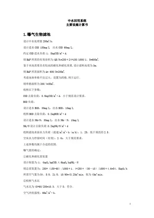
中水回用系统主要设施计算书1.曝气生物滤池设计中水处理量250m3/h,设计进水COD 150mg/L 出水COD 60mg/L,约定COD进水负荷:1。
5kgCOD/m3·d,则BAF所需的有效容积为:QS/N V=250*24*150/1000/1。
5=600m3,鉴于本池需要具有较高的碳化和硝化效果,设计滤料高度为3m,则BAF所需面积为A= 600/3=200m2,考虑池体单格不宜过大,设置为四格,利于运行。
则单格面积为200/4=50m2。
校核以下参数:COD去除负荷:0.9kgCOD/m3·d,小于规范设计要求。
BOD负荷:设计进水BOD:30mg/L,出水BOD:10mg/L校核BOD去除负荷:0.2kgBOD/m3·d设计进水NH3-N:30mg/L,出水NH3—N:10mg/LNH3-N设计去除负荷:0.2kgNH3-N/m3·d校核滤池表面水力负荷(滤速)m3/m2·h(m/h):1。
25,低于规范的2.5。
空床水力停留时间(有效):2.4h,大于规范要求。
上述参数均属于合适的范围。
曝气量的确定:①碳化和硝化需氧量设计取值为:1。
4kgO2/kgCOD,4.6kgO2/kgNH3—N则总需氧量为:250*(150-60)/1000*1。
4+250*(30—10)/1000*4.6=54。
5kgO2/h 所需空气量为54。
5/0。
21/0。
10/60=43.25m3/min,取为43m3/min。
②校核气水比气水比为43*60/250=10.3,大于8,符合。
空气冲洗强度:66m3/m2·h,则所需反冲洗气量:66*50/60=55m3/min。
水冲洗强度:22m3/m2·h;则所需反冲洗水量:22*50=1100m3/h,设计为3台泵,2用1备,单台流量550m3/h,扬程取为15m。
设计尺寸:单格L=8。
常用介质的设计计算

4、点击计算按钮输出结果:
5、点击 “计算书”按钮,软件自动生成计 算书
十一、 十一、管道损失计算
1、打开软件,手动输入流量、管道内径、 管道长度、介质密度、当量粗糙度及运动 粘度
2、运动粘度的调取:各种参数-水的运动粘 度
3、点击“ok”,自动计算出管路沿程阻力
4、调取局部阻力系数,根据管路上的管件 数计算局部阻力系数(加和)
七、保温层经济厚度计算
1、打开保温层经济厚度计算软件,选择保温材料
2、选择保温管线公称直径
3、选择保温管线介质温度,随后软件将自动计算出经济 厚度。
八、过热蒸汽温降计算
顺序将处于 “输入”前 的数据框中 的数据进行 手动输入, 没有“输入” 标示的位置 为软件自动 生成。
九、水管管道阻力计算
3、按照 推荐的 介质流 速手动 输入选 择的流 速
4、手动 输入介 质流量 和介质 比容
5、点击 计算按钮, 软件将自 动输出其 它数据: 管道内径 及其最大 和最小值
6、设计中还需考虑留有一定的余量,自行把 握。
五、管件当量计算
1、在蓝色阴 影区手动输入 管道外径和内 径:如、426 和13(注意单 位)
101209
水、蒸汽常用物性数据补充查询——潜热
二、量和单位转换
1、打开量和单位转换软件:
2、点击石油化工按钮:
3、选择动力粘度,在单位为CP中输入1
4、软件自动输出其它单位数据:
5、同理选择运动粘度(除此之外的导热系数也是 比较重要)厘斯:mm2/s
6、选择粘度转换——动力粘度-运动粘度
7、在弹出的对话框中手动输入动力粘度数 据:如25℃时水的粘度值。
2、在换热器形式中选择将要校核的换热器 形式:(见各种换热器形式动画)
Fluent计算多孔介质模型资料

广东省深圳市宝安区沙井辛养社区西部工业园 TEL:+86-755-3366-8888 FAX:+86-755-3366-0612Fluent计算多孔介质模型资料这是一个多孔介质例子,进口速度为0.01m/s,组份为液态水和氧气,其中氧气从多孔介质porous jump 渗透过去,如何看氧气在tissue中扩散的。
porous jump的face permeability1 a=e-8 m_2thickness 设为0.0001pressure jump coefficient为默认porous zone设置如下:direction vector 1, 1,viscous resistance 100 eachinertial resistance 100 eachporosity 0.1边界条件设置如下:Ab – wall - defaultBc – wall – defaultBe – porous jump – face permeability 1e-8, porous medium thickness0.0001Cd – outflow rating – 0.5De – wall – defaultDefault interior – interiorDefault interior001 – interiorDefault interior019 – interiorEf – wall - defaultFg – outflow rating – 1Fluid - porous zone - direction vector 1, 1, viscous resistance 100 each,inertial resistance 100 each, porosity 0.1Gh- wall - defaultHi – wall - defaultHk - porous jump same conditions as otherIj – outflow – 0.5Jk – wall – defaultKl – wall – defaultLa – velocity inlet – 0.01 m/s, temperature 300K, 0.5 mass fraction O2 Lfluid – porous zone - direction vector 1, 1, viscous resistance 100 each,inertial resistance 100 each, porosity 0.1Pipefluid – fluid – default (no porous zone)Models – species transport – water and oxygen mixtureVariations – different boundary conditions at top and bottom (outflow, wall ect)注意,其中porous zone在gambit中设置为fluid,在fluent中设置为porous zone边界条件设置如下:Ab – wall - defaultBc – wall – defaultBe – porous jump – face permeability 1e-8, porous medium thickness0.0001Cd – outflow rating – 0.5De – wall – defaultDefault interior – interiorDefault interior001 – interiorDefault interior019 – interiorEf – wall - defaultFg – outflow rating – 1Fluid - porous zone - direction vector 1, 1, viscous resistance 100 each,inertial resistance 100 each, porosity 0.1Gh- wall - defaultHi – wall - defaultHk - porous jump same conditions as otherIj – outflow – 0.5Jk – wall – defaultKl – wall – defaultLa – velocity inlet – 0.01 m/s, temperature 300K, 0.5 mass fraction O2 Lfluid – porous zone - direction vector 1, 1, viscous resistance 100 each,inertial resistance 100 each, porosity 0.1Pipefluid – fluid – default (no porous zone)Models – species transport – water and oxygen mixtureVariations – different boundary conditions at top and bottom (outflow, wall ect) 注意,其中porous zone在gambit中设置为fluid,在fluent中设置为porous zone。
fluent中多孔介质设置问题和算例

经过痛苦的一段经历,终于将局部问题真相大白,为了使保位同仁不再经过我之痛苦,现在将本人多孔介质经验公布如下,希望各位能加精:1。
Gambit中划分网格之后,定义需要做为多孔介质的区域为fl uid,与缺省的fl uid分别开来,再定义其名称,我习惯将名称定义为po rous;2。
在fluen t中定义边界条件de fine-bounda ry condit ion-porous(刚定义的名称),将其设置边界条件为fl uid,点击set按钮即弹出与f luid边界条件一样的对话框,选中poro us zone 与l a mina r复选框,再点击por ous zone标签即出现一个带有滚动条的界面;3。
porous zone设置方法:1)定义矢量:二维定义一个矢量,第二个矢量方向不用定义,是与第一个矢量方向正交的;三维定义二个矢量,第三个矢量方向不用定义,是与第一、二个矢量方向正交的;(如何知道矢量的方向:打开grid图,看看X,Y,Z的方向,如果是X向,矢量为1,0,0,同理Y向为0,1,0,Z向为0,0,1,如果所需要的方向与坐标轴正向相反,则定义矢量为负)圆锥坐标与球坐标请参考f luen t帮助。
2)定义粘性阻力1/a与内部阻力C2:请参看本人上一篇博文“终于搞清fl uent中多孔粘性阻力与内部阻力的计算方法”,此处不赘述;3)如果了定义粘性阻力1/a与内部阻力C2,就不用定义C1与C0,因为这是两种不同的定义方法,C1与C0只在幂率模型中出现,该处保持默认就行了;4)定义孔隙率p o rous ity,默认值1表示全开放,此值按实验测值填写即可。
完了,其他设置与普通k-e或RSM相同。
总结一下,与君共享!Tutori al 7. Modeli ng Flow Throug h Porous MediaIntrod uctio nMany indust rialapplic ation s involv e the modeli ng of flow throug h porous media, such as filters, cataly st beds, and packin g. This tutori al illust rates how to set up and solvea proble m involv ing gas flow throug h porous media.The indust rialproble m solved here involv es gas flow throug h a cataly tic conver ter. Cataly tic conver tersare common ly used to purify emissi ons from gasoli ne and diesel engine s by conver tingenviro nment allyhazard ous exhaus t emissi ons to accept ablesubsta nces.Exampl es of such emissi ons includ e carbon monoxi de (CO), nitrog en oxides (NOx), and unburn ed hydroc arbon fuels. Theseexhaus t gas emissi ons are forced throug h a substr ate, whichis a cerami c struct ure coated with a metalcataly st such as platin um or pallad ium.The nature of the exhaus t gas flow is a very import ant factor in determ ining the perfor mance of the cataly tic conver ter. Of partic ularimport anceis the pressu re gradie nt and veloci ty distri butio n throug h the substr ate. HenceCFD analys is is used to design effici ent cataly tic conver ters: by modeli ng the exhaus t gas flow, the pressu re drop and the unifor mityof flow throug h the substr ate can be determ ined. In this tutori al, FLUENT is used to modelthe flow of nitrog en gas throug h a cataly tic conver ter geomet ry, so that the flow field struct ure may be analyz ed.This tutori al demons trate s how to do the follow ing:_ Set up a porous zone for the substr ate with approp riate resist ances._ Calcul ate a soluti on for gas flow throug h the cataly tic conver ter usingthe pressu re basedsolver. _ Plot pressu re and veloci ty distri butio n on specif ied planes of the geomet ry._ Determ ine the pressu re drop throug h the substr ate and the degree of non-unifor mityof flow throug h crosssectio ns of the geomet ry usingX-Y plotsand numeri cal report s.Proble m Descri ptionThe cataly tic conver ter modele d here is shownin Figure 7.1. The nitrog en flowsin throug h the inletwith a unifor m veloci ty of 22.6 m/s, passes throug h a cerami c monoli th substr ate with square shaped channe ls, and then exitsthroug h the outlet.Whilethe flow in the inletand outlet sectio ns is turbul ent, the flow throug h the substr ate is lamina r and is charac teriz ed by inerti al and viscou s loss coeffi cient s in the flow (X) direct ion. The substr ate is imperm eable in otherdirect ions, whichis modele d usingloss coeffi cients whosevalues are threeorders of magnit ude higher than in the X direct ion.Setupand Soluti onStep 1: Grid1. Read the mesh file (cataly tic conver ter.msh).File /Read /Case...2. Checkthe grid. Grid /CheckFLUENT will perfor m variou s checks on the mesh and report the progre ss in the consol e. Make sure that the minimu m volume report ed is a positi ve number.3. Scalethe grid.Grid! Scale...(a) Select mm from the Grid Was Create d In drop-down list.(b) Clickthe Change Length Unitsbutton. All dimens ionswill now be shownin millim eters.(c) ClickScaleand closethe ScaleGrid panel.4. Displa y the mesh. Displa y /Grid...(a) Make sure that inlet, outlet, substr ate-wall, and wall are select ed in the Surfac es select ion list.(b) ClickDispla y.(c) Rotate the view and zoom in to get the displa y shownin Figure 7.2.(d) Closethe Grid Displa y panel.The hex mesh on the geomet ry contai ns a totalof 34,580 cells.Step 2: Models1. Retain the defaul t solver settin gs. Define /Models /Solver...2. Select the standa rd k-ε turbul encemodel.Define/ Models /Viscou s...Step 3: Materi als1. Add nitrog en to the list of fluid materi als by copyin g it from the Fluent Databa se for materi als. Define /Materi als...(a) Clickthe Fluent Databa se... button to open the Fluent Databa se Materi als panel.i. Select nitrog en (n2) from the list of Fluent FluidMateri als.ii. ClickCopy to copy the inform ation for nitrog en to your list of fluid materi als. iii. Closethe Fluent Databa se Materi als panel.(b) Closethe Materi als panel.Step 4: Bounda ry Condit ions.Define /Bounda ry Condit ions...1. Set the bounda ry condit ionsfor the fluid(fluid).(a) Select nitrog en from the Materi al Name drop-down list.(b) ClickOK to closethe Fluidpanel.2. Set the bounda ry condit ionsfor the substr ate (substr ate).(a) Select nitrog en from the Materi al Name drop-down list.(b) Enable the Porous Zone option to activa te the porous zone model.(c) Enable the Lamina r Zone option to solvethe flow in the porous zone withou t turbul ence.(d) Clickthe Porous Zone tab.i. Make sure that the princi pal direct ion vector s are set as shownin Table7.1. Use the scroll bar to access the fields that are not initia lly visibl e in the panel.ii. Enterthe values in Table7.2 for the Viscou s Resist anceand Inerti al Resist ance. Scroll down to access the fields that are not initia lly visibl e in the panel.(e) ClickOK to closethe Fluidpanel.3. Set the veloci ty and turbul encebounda ry condit ionsat the inlet(inlet).(a) Enter22.6 m/s for the Veloci ty Magnit ude.(b) Select Intens ity and Hydrau lic Diamet er from the Specif ication Method dropdo wn list in the Turbul encegroupbox.(c) Retain the defaul t valueof 10% for the Turbul ent Intens ity.(d) Enter42 mm for the Hydrau lic Diamet er.(e) ClickOK to closethe Veloci ty Inletpanel.4. Set the bounda ry condit ionsat the outlet (outlet).(a) Retain the defaul t settin g of 0 for GaugePressu re.(b) Select Intens ity and Hydrau lic Diamet er from the Specif ication Method dropdo wn list in the Turbul encegroupbox.(c) Enter5% for the Backfl ow Turbul ent Intens ity.(d) Enter42 mm for the Backfl ow Hydrau lic Diamet er.(e) ClickOK to closethe Pressu re Outlet panel.5. Retain the defaul t bounda ry condit ionsfor the walls(substr ate-wall and wall) and closethe Bounda ry Condit ionspanel.Step 5: Soluti on1. Set the soluti on parame ters.Solve/Contro ls /Soluti on...(a) Retain the defaul t settin gs for Under-Relaxa tionFactor s.(b) Select Second OrderUpwind from the Moment um drop-down list in the Discre tizat ion groupbox.(c) ClickOK to closethe Soluti on Contro ls panel.2. Enable the plotti ng of residu als during the calcul ation. Solve/Monito rs /Residu al...(a) Enable Plot in the Option s groupbox.(b) ClickOK to closethe Residu al Monito rs panel.3. Enable the plotti ng of the mass flow rate at the outlet.Solve/ Monito rs /Surfac e...(a) Set the Surfac e Monito rs to 1.(b) Enable the Plot and Writeoption s for monito r-1, and clickthe Define... button to open the Define Surfac e Monito r panel.i. Select Mass Flow Rate from the Report Type drop-down list.ii. Select outlet from the Surfac es select ion list.iii. ClickOK to closethe Define Surfac e Monito rs panel.(c) ClickOK to closethe Surfac e Monito rs panel.4. Initia lizethe soluti on from the inlet.Solve/Initia lize/Initia lize...(a) Select inletfrom the Comput e From drop-down list.(b) ClickInit and closethe Soluti on Initia lizat ion panel.5. Save the case file (cataly tic conver ter.cas). File /Write/Case...6. Run the calcul ation by reques ting100 iterat ions.Solve/Iterat e...(a) Enter100 for the Number of Iterat ions.(b) ClickIterat e.The FLUENT calcul ation will conver ge in approx imate ly 70 iterat ions. By this pointthe mass flow rate monito r has attend ed out, as seen in Figure 7.3.(c) Closethe Iterat e panel.7. Save the case and data files(cataly tic conver ter.cas and cataly tic conver ter.dat).File /Write/Case & Data...Note: If you choose a file name that alread y exists in the curren t folder, FLUENTwill prompt you for confir matio n to overwr ite the file.Step 6: Post-proces sing1. Create a surfac e passin g throug h the center linefor post-proces singpurpos es.Surfac e/Iso-Surfac e...(a) Select Grid... and Y-Coordi natefrom the Surfac e of Consta nt drop-down lists.(b) ClickComput e to calcul ate the Min and Max values.(c) Retain the defaul t valueof 0 for the Iso-Values.(d) Entery=0 for the New Surfac e Name.(e) ClickCreate.2. Create cross-sectio nal surfac es at locati ons on either side of the substr ate, as well as at its center.Surfac e /Iso-Surfac e...(a) Select Grid... and X-Coordi natefrom the Surfac e of Consta nt drop-down lists.(b) ClickComput e to calcul ate the Min and Max values.(c) Enter95 for Iso-Values.(d) Enterx=95 for the New Surfac e Name.(e) ClickCreate.(f) In a simila r manner, create surfac es namedx=130 and x=165 with Iso-Values of 130 and 165, respec tivel y. Closethe Iso-Surfac e panelafterall the surfac es have been create d.3. Create a line surfac e for the center lineof the porous media.Surfac e /Line/Rake...(a) Enterthe coordi nates of the line underEnd Points, usingthe starti ng coordi nateof (95, 0, 0) and an ending coordi nateof (165, 0, 0), as shown.(b) Enterporous-cl for the New Surfac e Name.(c) ClickCreate to create the surfac e.(d) Closethe Line/Rake Surfac e panel.4. Displa y the two wall zones(substr ate-wall and wall). Displa y /Grid...(a) Disabl e the Edgesoption.(b) Enable the Facesoption.(c) Desele ct inletand outlet in the list underSurfac es, and make sure that only substr ate-wall and wall are select ed.(d) ClickDispla y and closethe Grid Displa y panel.(e) Rotate the view and zoom so that the displa y is simila r to Figure 7.2.5. Set the lighti ng for the displa y. Displa y /Option s...(a) Enable the Lights On option in the Lighti ng Attrib utesgroupbox.(b) Retain the defaul t select ion of Gouran d in the Lighti ng drop-down list.(c) ClickApplyand closethe Displa y Option s panel.6. Set the transp arenc y parame ter for the wall zones(substr ate-wall and wall).Displa y/Scene...(a) Select substr ate-wall and wall in the Namesselect ion list.(b) Clickthe Displa y... button underGeomet ry Attrib utesto open the Displa y Proper tiespanel.i. Set the Transp arenc y slider to 70.ii. ClickApplyand closethe Displa y Proper tiespanel.(c) ClickApplyand then closethe SceneDescri ption panel.7. Displa y veloci ty vector s on the y=0 surfac e.Displa y /Vector s...(a) Enable the Draw Grid option. The Grid Displa y panelwill open.i. Make sure that substr ate-wall and wall are select ed in the list underSurfac es.ii. ClickDispla y and closethe Displa y Grid panel.(b) Enter5 for the Scale.(c) Set Skip to 1.(d) Select y=0 from the Surfac es select ion list.(e) ClickDispla y and closethe Vector s panel.The flow patter n showsthat the flow enters the cataly tic conver ter as a jet, with recirc ulati on on either side of the jet. As it passes throug h the porous substr ate, it decele rates and straig htens out, and exhibi ts a more unifor m veloci ty distri butio n.This allows the metalcataly st presen t in the substr ate to be more effect ive.Figure 7.4: Veloci ty Vector s on the y=0 Plane8. Displa y filled contou rs of static pressu re on the y=0 plane.Displa y /Contou rs...(a) Enable the Filled option.(b) Enable the Draw Grid option to open the Displa y Grid panel.i. Make sure that substr ate-wall and wall are select ed in the list underSurfac es.ii. ClickDispla y and closethe Displa y Grid panel.(c) Make sure that Pressu re... and Static Pressu re are select ed from the Contou rs of drop-down lists.(d) Select y=0 from the Surfac es select ion list.(e) ClickDispla y and closethe Contou rs panel.Figure 7.5: Contou rs of the Static Pressu re on the y=0 planeThe pressu re change s rapidl y in the middle sectio n, wherethe fluid veloci ty change s as it passes throug h the porous substr ate. The pressu re drop can be high, due to the inerti al and viscou s resist anceof the porous media. Determ ining this pressu re drop is a goal of CFD analys is. In the next step, you will learnhow to plot the pressu re drop alongthe center lineof the substr ate.9. Plot the static pressu re across the line surfac e porous-cl.Plot /XY Plot...(a) Make sure that the Pressu re... and Static Pressu re are select ed from the Y Axis Functi on drop-down lists.(b) Select porous-cl from the Surfac es select ion list.(c) ClickPlot and closethe Soluti on XY Plot panel.Figure 7.6: Plot of the Static Pressu re on the porous-cl Line Surfac eIn Figure 7.6, the pressu re drop across the porous substr ate can be seen to be roughl y 300 Pa.10. Displa y filled contou rs of the veloci ty in the X direct ion on the x=95, x=130 and x=165 surfac es.Displa y /Contou rs...(a) Disabl e the Global Rangeoption.(b) Select Veloci ty... and X Veloci ty from the Contou rs of drop-down lists.(c) Select x=130, x=165, and x=95 from the Surfac es select ion list, and desele ct y=0.(d) ClickDispla y and closethe Contou rs panel.The veloci ty profil e become s more unifor m as the fluid passes throug h the porous media. The veloci ty is very high at the center (the area in red) just before the nitrog en enters the substr ate and then decrea ses as it passes throug h and exitsthe substr ate. The area in green, whichcorres ponds to a modera te veloci ty, increa ses in extent.Figure 7.7: Contou rs of the X Veloci ty on the x=95, x=130, and x=165 Surfac es11. Use numeri cal report s to determ ine the averag e, minimu m, and maximu m of the veloci tydistri butio n before and afterthe porous substr ate.Report /Surfac e Integr als...(a) Select Mass-Weight ed Averag e from the Report Type drop-down list.(b) Select Veloci ty and X Veloci ty from the FieldVariab le drop-down lists.(c) Select x=165 and x=95 from the Surfac es select ion list.(d) ClickComput e.(e) Select FacetMinimu m from the Report Type drop-down list and clickComput e again.(f) Select FacetMaximu m from the Report Type drop-down list and clickComput e again.(g) Closethe Surfac e Integr als panel.The numeri cal report of averag e, maximu m and minimu m veloci ty can be seen in the main FLUENT consol e, as shownin the follow ing exampl e:The spread betwee n the averag e, maximu m, and minimu m values for X veloci ty givesthe degree to whichthe veloci ty distri butio n is non-unifor m. You can also use thesenumber s to calcul ate the veloci ty ratio(i.e., the maximu m veloci ty divide d by the mean veloci ty) and the spaceveloci ty (i.e., the produc t of the mean veloci ty and the substr ate length).Custom field functi ons and UDFs can be also used to calcul ate more comple x measur es ofnon-unifor mity, such as the standa rd deviat ion and the gammaunifor mityindex.Summar yIn this tutori al, you learne d how to set up and solvea proble m involv ing gas flow throug h porous mediain FLUENT. You also learne d how to perfor m approp riate post-proces singto invest igate the flow field, determ ine the pressu re drop across the porous mediaand non-unifor mityof the veloci ty distri butio n as the fluid goes throug h the porous media.Furthe r Improv ement sThis tutori al guides you throug h the stepsto reachan initia l soluti on. You may be able to obtain a more accura te soluti on by usingan approp riate higher-orderdiscre tizat ion scheme and by adapti ng the grid. Grid adapti on can also ensure that the soluti on is indepe ndent of the grid. Thesestepsare demons trate d in Tutori al 1.。
多介质环境目标值-换算公式
多介质环境目标值-换算公式化学物质在没有环境空气质量标准和居住区大气环境质量标准情况下,推荐大家采用AMEG值,主要计算公式如下:美国环保局于1977年公布了该局工业环境实验室用模式推算出来的六百多中化学物质在各种环境介质(空气、水、土壤)中的限定值。
又于1980年对其进行了增补,并建议将其作为环境评价的依据值。
这些限定值被称为多介质环境目标值(Multimeedia Environmental Goal,MEG)。
所有目标值都是在最基本的毒性数据基础上,以统一模式推算的,系统性和可比性好。
因而,多介质环境目标值虽然不具法律效力,却可以作为环境评价的依据。
目前,它已在美国环境影响评价中广泛应用。
●以毒理学数据LD50为基础的计算公式为:AMEG=0.107×LD50/1000式中:AMEG-空气环境目标值(相当于居住区空气中日平均最高容许浓度,mg/m3) LD50-大鼠经口给毒的半数致死剂量以环氧乙烷为例,LD50--330mg/kg,计算得AMEG值= 0.04mg/m3,因此推荐居住区环境空气中环氧乙烷最高容许浓度为0.04 mg/m3(日平均值),根据《环境影响评价技术导则-大气环境》(HJ/T2.2-93)“8.1.2.5 如无法获得8.1.2.1中所述的监测资料,一次取样、日、月、季(或期)、年平均值可按1、0.33、0.20、0.14、0.12的比例关系换算”,则计算得相应1小时平均值为0.11 mg/m3。
●以阙限值为基础的计算公式为:AMEG=阙限值/420式中:AMEG-空气环境目标值(相当于居住区空气中日平均最高容许浓度,mg/m3) 阙限值-美国政府工业卫生学家会议(ACGIH)制定的车间空气容许浓度,即每周工作5天,每天工作8小时条件下,成年工人可以耐受的化学物质在空气中的时间加权平均浓度,mg/m3●以健康影响为依据的空气介质排放环境目标值(DMEGAH)可按下式计算:DMEGAH (μg/m3) = 45× LD50式中:DMEGAH——允许排放浓度,LD50——化学物质的毒理数据,一般取大鼠经口给毒的LD50,若无此数据,可取与其接近的毒理学数据。
压力容器设计计算书(MMF+AC+MB+SF)
原始数据
Flow(m /h)
3
活性炭过滤器
原始数据
8.5 Flow(m /h)
3
10
MMF 桶体直径 7 过滤流速(m/h) 1243.73 计算桶体直径(mm) 1200.00 修正桶体直径(mm) 7.52 修正流速(m/h) MMF 桶体高度 填充总高度(mm) 膨胀系数 膨胀高度(mm) 修正膨胀高度(mm) 上水帽高度(mm) 下水帽高度(mm) 过滤器总高度(mm) MMF 反洗水量 LV(m/h) 反洗流量(m /h) 正洗流速(m/h) 正洗流量(m3/h) 反洗时间(min) 静置时间(min) 正洗时间(min) 反洗总时间(min) 反洗水量(m3) 正洗水量(m3) 总水量(m3)
3
15 14.25 10 10 10 10 10 30 2.37 1.67 4.04
1200 0.4 480 500 100 100 1900
1200 9.22 7 8.5 10 10 10 30 3.20 1.42 4.62
LV(m/h) 反洗流量(m /h) 正洗流速(m/h) 正洗流量(m3/h) 反洗时间(min) 静置时间(min) 正洗时间(min) 反洗总时间(min) 反洗水量(m3) 正洗水量(m3) 总水量(m3)
3
ACF 桶体直径 10 过滤流速(m/h) 1128.67 计算桶体直径(mm) 1100.00 修正桶体直径(mm) 10.53 修正流速(m/h) ACF 桶体高度 填充总高度(mm) 膨胀系数 膨胀高度(mm) 修正膨胀高度(mm) 上水帽高度(mm) 下水帽高度(mm) 过滤器总高度(mm) ACF 反洗水量
(完整word版)fluent中多孔介质设置问题和算例
经过痛苦的一段经历,终于将局部问题真相大白,为了使保位同仁不再经过我之痛苦,现在将本人多孔介质经验公布如下,希望各位能加精:1。
Gambit中划分网格之后,定义需要做为多孔介质的区域为fluid,与缺省的fluid分别开来,再定义其名称,我习惯将名称定义为porous;2。
在fluent中定义边界条件define-boundary condition-porous(刚定义的名称),将其设置边界条件为fluid,点击set按钮即弹出与fluid边界条件一样的对话框,选中porous zone与laminar复选框,再点击porous zone标签即出现一个带有滚动条的界面;3。
porous zone设置方法:1)定义矢量:二维定义一个矢量,第二个矢量方向不用定义,是与第一个矢量方向正交的;三维定义二个矢量,第三个矢量方向不用定义,是与第一、二个矢量方向正交的;(如何知道矢量的方向:打开grid图,看看X,Y,Z的方向,如果是X向,矢量为1,0,0,同理Y向为0,1,0,Z向为0,0,1,如果所需要的方向与坐标轴正向相反,则定义矢量为负)圆锥坐标与球坐标请参考fluent帮助。
2)定义粘性阻力1/a与内部阻力C2:请参看本人上一篇博文“终于搞清fluent中多孔粘性阻力与内部阻力的计算方法”,此处不赘述;3)如果了定义粘性阻力1/a与内部阻力C2,就不用定义C1与C0,因为这是两种不同的定义方法,C1与C0只在幂率模型中出现,该处保持默认就行了;4)定义孔隙率porousity,默认值1表示全开放,此值按实验测值填写即可。
完了,其他设置与普通k-e或RSM相同。
总结一下,与君共享!Tutorial 7. Modeling Flow Through Porous MediaIntroductionMany industrial applications involve the modeling of flow through porous media, such as filters, catalyst beds, and packing. This tutorial illustrates how to set up and solve a problem involving gas flow through porous media.The industrial problem solved here involves gas flow through a catalytic converter. Catalytic converters are commonly used to purify emissions from gasoline and diesel engines by converting environmentally hazardous exhaust emissions to acceptable substances.Examples of such emissions include carbon monoxide (CO), nitrogen oxides (NOx), and unburned hydrocarbon fuels. These exhaust gas emissions are forced through a substrate, which is a ceramic structure coated with a metal catalyst such as platinum or palladium.The nature of the exhaust gas flow is a very important factor in determining the performance of the catalytic converter. Of particular importance is the pressure gradient and velocity distribution through the substrate. Hence CFD analysis is used to design efficient catalytic converters: by modeling the exhaust gas flow, the pressure drop and the uniformity of flow through the substrate can be determined. In this tutorial, FLUENT is used to model the flow of nitrogen gas through a catalytic converter geometry, so that the flow field structure may be analyzed.This tutorial demonstrates how to do the following:_ Set up a porous zone for the substrate with appropriate resistances._ Calculate a solution for gas flow through the catalytic converter using the pressure based solver. _ Plot pressure and velocity distribution on specified planes of the geometry._ Determine the pressure drop through the substrate and the degree of non-uniformity of flow through cross sections of the geometry using X-Y plots and numerical reports.Problem DescriptionThe catalytic converter modeled here is shown in Figure 7.1. The nitrogen flows in through the inlet with a uniform velocity of 22.6 m/s, passes through a ceramic monolith substrate with square shaped channels, and then exits through the outlet.While the flow in the inlet and outlet sections is turbulent, the flow through the substrate is laminar and is characterized by inertial and viscous loss coefficients in the flow (X) direction. The substrate is impermeable in other directions, which is modeled using loss coefficients whose values are three orders of magnitude higher than in the X direction.Setup and SolutionStep 1: Grid1. Read the mesh file (catalytic converter.msh).File /Read /Case...2. Check the grid. Grid /CheckFLUENT will perform various checks on the mesh and report the progress in the console. Make sure that the minimum volume reported is a positive number.3. Scale the grid.Grid! Scale...(a) Select mm from the Grid Was Created In drop-down list.(b) Click the Change Length Units button. All dimensions will now be shown in millimeters.(c) Click Scale and close the Scale Grid panel.4. Display the mesh. Display /Grid...(a) Make sure that inlet, outlet, substrate-wall, and wall are selected in the Surfaces selection list.(b) Click Display.(c) Rotate the view and zoom in to get the display shown in Figure 7.2.(d) Close the Grid Display panel.The hex mesh on the geometry contains a total of 34,580 cells.Step 2: Models1. Retain the default solver settings. Define /Models /Solver...2. Select the standard k-ε turbulence model. Define/ Models /Viscous...Step 3: Materials1. Add nitrogen to the list of fluid materials by copying it from the Fluent Database for materials.Define /Materials...(a) Click the Fluent Database... button to open the Fluent Database Materials panel.i. Select nitrogen (n2) from the list of Fluent Fluid Materials.ii. Click Copy to copy the information for nitrogen to your list of fluid materials. iii. Close the Fluent Database Materials panel.(b) Close the Materials panel.Step 4: Boundary Conditions. Define /Boundary Conditions...1. Set the boundary conditions for the fluid (fluid).(a) Select nitrogen from the Material Name drop-down list.(b) Click OK to close the Fluid panel.2. Set the boundary conditions for the substrate (substrate).(a) Select nitrogen from the Material Name drop-down list.(b) Enable the Porous Zone option to activate the porous zone model.(c) Enable the Laminar Zone option to solve the flow in the porous zone without turbulence.(d) Click the Porous Zone tab.i. Make sure that the principal direction vectors are set as shown in Table7.1. Use the scroll bar to access the fields that are not initially visible in the panel.ii. Enter the values in Table 7.2 for the Viscous Resistance and Inertial Resistance. Scroll down to access the fields that are not initially visible in the panel.(e) Click OK to close the Fluid panel.3. Set the velocity and turbulence boundary conditions at the inlet (inlet).(a) Enter 22.6 m/s for the Velocity Magnitude.(b) Select Intensity and Hydraulic Diameter from the Specification Method dropdown list in the Turbulence group box.(c) Retain the default value of 10% for the Turbulent Intensity.(d) Enter 42 mm for the Hydraulic Diameter.(e) Click OK to close the Velocity Inlet panel.4. Set the boundary conditions at the outlet (outlet).(a) Retain the default setting of 0 for Gauge Pressure.(b) Select Intensity and Hydraulic Diameter from the Specification Method dropdown list in the Turbulence group box.(c) Enter 5% for the Backflow Turbulent Intensity.(d) Enter 42 mm for the Backflow Hydraulic Diameter.(e) Click OK to close the Pressure Outlet panel.5. Retain the default boundary conditions for the walls (substrate-wall and wall) and close the Boundary Conditions panel.Step 5: Solution1. Set the solution parameters. Solve /Controls /Solution...(a) Retain the default settings for Under-Relaxation Factors.(b) Select Second Order Upwind from the Momentum drop-down list in the Discretization group box.(c) Click OK to close the Solution Controls panel.2. Enable the plotting of residuals during the calculation. Solve/Monitors /Residual...(a) Enable Plot in the Options group box.(b) Click OK to close the Residual Monitors panel.3. Enable the plotting of the mass flow rate at the outlet.Solve / Monitors /Surface...(a) Set the Surface Monitors to 1.(b) Enable the Plot and Write options for monitor-1, and click the Define... button to open the Define Surface Monitor panel.i. Select Mass Flow Rate from the Report Type drop-down list.ii. Select outlet from the Surfaces selection list.iii. Click OK to close the Define Surface Monitors panel.(c) Click OK to close the Surface Monitors panel.4. Initialize the solution from the inlet. Solve /Initialize /Initialize...(a) Select inlet from the Compute From drop-down list.(b) Click Init and close the Solution Initialization panel.5. Save the case file (catalytic converter.cas). File /Write /Case...6. Run the calculation by requesting 100 iterations. Solve /Iterate...(a) Enter 100 for the Number of Iterations.(b) Click Iterate.The FLUENT calculation will converge in approximately 70 iterations. By this point the mass flow rate monitor has attended out, as seen in Figure 7.3.(c) Close the Iterate panel.7. Save the case and data files (catalytic converter.cas and catalytic converter.dat).File /Write /Case & Data...Note: If you choose a file name that already exists in the current folder, FLUENTwill prompt you for confirmation to overwrite the file.Step 6: Post-processing1. Create a surface passing through the centerline for post-processing purposes.Surface/Iso-Surface...(a) Select Grid... and Y-Coordinate from the Surface of Constant drop-down lists.(b) Click Compute to calculate the Min and Max values.(c) Retain the default value of 0 for the Iso-Values.(d) Enter y=0 for the New Surface Name.(e) Click Create.2. Create cross-sectional surfaces at locations on either side of the substrate, as well as at its center.Surface /Iso-Surface...(a) Select Grid... and X-Coordinate from the Surface of Constant drop-down lists.(b) Click Compute to calculate the Min and Max values.(c) Enter 95 for Iso-Values.(d) Enter x=95 for the New Surface Name.(e) Click Create.(f) In a similar manner, create surfaces named x=130 and x=165 with Iso-Values of 130 and 165, respectively. Close the Iso-Surface panel after all the surfaces have been created.3. Create a line surface for the centerline of the porous media.Surface /Line/Rake...(a) Enter the coordinates of the line under End Points, using the starting coordinate of (95, 0, 0) and an ending coordinate of (165, 0, 0), as shown.(b) Enter porous-cl for the New Surface Name.(c) Click Create to create the surface.(d) Close the Line/Rake Surface panel.4. Display the two wall zones (substrate-wall and wall). Display /Grid...(a) Disable the Edges option.(b) Enable the Faces option.(c) Deselect inlet and outlet in the list under Surfaces, and make sure that only substrate-wall and wall are selected.(d) Click Display and close the Grid Display panel.(e) Rotate the view and zoom so that the display is similar to Figure 7.2.5. Set the lighting for the display. Display /Options...(a) Enable the Lights On option in the Lighting Attributes group box.(b) Retain the default selection of Gourand in the Lighting drop-down list.(c) Click Apply and close the Display Options panel.6. Set the transparency parameter for the wall zones (substrate-wall and wall).Display/Scene...(a) Select substrate-wall and wall in the Names selection list.(b) Click the Display... button under Geometry Attributes to open the Display Properties panel.i. Set the Transparency slider to 70.ii. Click Apply and close the Display Properties panel.(c) Click Apply and then close the Scene Description panel.7. Display velocity vectors on the y=0 surface.Display /Vectors...(a) Enable the Draw Grid option. The Grid Display panel will open.i. Make sure that substrate-wall and wall are selected in the list under Surfaces.ii. Click Display and close the Display Grid panel.(b) Enter 5 for the Scale.(c) Set Skip to 1.(d) Select y=0 from the Surfaces selection list.(e) Click Display and close the Vectors panel.The flow pattern shows that the flow enters the catalytic converter as a jet, with recirculation on either side of the jet. As it passes through the porous substrate, it decelerates and straightens out, and exhibits a more uniform velocity distribution.This allows the metal catalyst present in the substrate to be more effective.Figure 7.4: Velocity Vectors on the y=0 Plane8. Display filled contours of static pressure on the y=0 plane.Display /Contours...(a) Enable the Filled option.(b) Enable the Draw Grid option to open the Display Grid panel.i. Make sure that substrate-wall and wall are selected in the list under Surfaces.ii. Click Display and close the Display Grid panel.(c) Make sure that Pressure... and Static Pressure are selected from the Contours of drop-down lists.(d) Select y=0 from the Surfaces selection list.(e) Click Display and close the Contours panel.Figure 7.5: Contours of the Static Pressure on the y=0 planeThe pressure changes rapidly in the middle section, where the fluid velocity changes as it passes through the porous substrate. The pressure drop can be high, due to the inertial and viscous resistance of the porous media. Determining this pressure drop is a goal of CFD analysis. In the next step, you will learn how to plot the pressure drop along the centerline of the substrate.9. Plot the static pressure across the line surface porous-cl.Plot /XY Plot...(a) Make sure that the Pressure... and Static Pressure are selected from the Y Axis Function drop-down lists.(b) Select porous-cl from the Surfaces selection list.(c) Click Plot and close the Solution XY Plot panel.Figure 7.6: Plot of the Static Pressure on the porous-cl Line SurfaceIn Figure 7.6, the pressure drop across the porous substrate can be seen to be roughly 300 Pa.10. Display filled contours of the velocity in the X direction on the x=95, x=130 and x=165 surfaces.Display /Contours...(a) Disable the Global Range option.(b) Select Velocity... and X Velocity from the Contours of drop-down lists.(c) Select x=130, x=165, and x=95 from the Surfaces selection list, and deselect y=0.(d) Click Display and close the Contours panel.The velocity profile becomes more uniform as the fluid passes through the porous media. The velocity is very high at the center (the area in red) just before the nitrogen enters the substrate and then decreases as it passes through and exits the substrate. The area in green, which corresponds to a moderate velocity, increases in extent.Figure 7.7: Contours of the X Velocity on the x=95, x=130, and x=165 Surfaces11. Use numerical reports to determine the average, minimum, and maximum of the velocity distribution before and after the porous substrate.Report /Surface Integrals...(a) Select Mass-Weighted Average from the Report Type drop-down list.(b) Select Velocity and X Velocity from the Field Variable drop-down lists.(c) Select x=165 and x=95 from the Surfaces selection list.(d) Click Compute.(e) Select Facet Minimum from the Report Type drop-down list and click Compute again.(f) Select Facet Maximum from the Report Type drop-down list and click Compute again.(g) Close the Surface Integrals panel.The numerical report of average, maximum and minimum velocity can be seen in the main FLUENT console, as shown in the following example:The spread between the average, maximum, and minimum values for X velocity gives the degree to which the velocity distribution is non-uniform. You can also use these numbers to calculate the velocity ratio (i.e., the maximum velocity divided by the mean velocity) and the space velocity (i.e., the product of the mean velocity and the substrate length).Custom field functions and UDFs can be also used to calculate more complex measures ofnon-uniformity, such as the standard deviation and the gamma uniformity index.SummaryIn this tutorial, you learned how to set up and solve a problem involving gas flow through porous media in FLUENT. You also learned how to perform appropriate post-processing to investigate the flow field, determine the pressure drop across the porous media and non-uniformity of the velocity distribution as the fluid goes through the porous media.Further ImprovementsThis tutorial guides you through the steps to reach an initial solution. You may be able to obtain a more accurate solution by using an appropriate higher-order discretization scheme and by adapting the grid. Grid adaption can also ensure that the solution is independent of the grid. These steps aredemonstrated in Tutorial 1.。
fluent中多孔介质设置问题和算例
经过痛苦的一段经历,终于将局部问题真相大白,为了使保位同仁不再经过我之痛苦,现在将本人多孔介质经验公布如下,希望各位能加精:1。
Gambit 中划分网格之后,定义需要做为多孔介质的区域为fluid, 与缺省的fluid 分别开来,再定义其名称,我习惯将名称定义为porous;2。
在fluent 中定义边界条件define-boundary condition-porous(刚定义的名称),将其设置边界条件为fluid, 点击set 按钮即弹出与fluid 边界条件一样的对话框,选中porous zone 与laminar 复选框, 再点击porous zone 标签即出现一个带有滚动条的界面;3。
porous zone 设置方法:1)定义矢量:二维定义一个矢量,第二个矢量方向不用定义,是与第一个矢量方向正交的;三维定义二个矢量,第三个矢量方向不用定义,是与第一、二个矢量方向正交的;(如何知道矢量的方向:打开grid 图,看看X,Y,Z 的方向,如果是X 向,矢量为1,0,0, 同理Y 向为0,1,0 ,Z 向为0,0,1, 如果所需要的方向与坐标轴正向相反,则定义矢量为负)圆锥坐标与球坐标请参考fluent 帮助。
2)定义粘性阻力1/a 与内部阻力C2:请参看本人上一篇博文“ 终于搞清fluent 中多孔粘性阻力与内部阻力的计算方法”,此处不赘述;3)如果了定义粘性阻力1/a 与内部阻力C2,就不用定义C1 与C0,因为这是两种不同的定义方法,C1与C0 只在幂率模型中出现,该处保持默认就行了;4)定义孔隙率porousity ,默认值1 表示全开放,此值按实验测值填写即可。
完了,其他设置与普通k-e 或RSM相同。
总结一下,与君共享!Tutorial 7. Modeling Flow Through Porous MediaIntroductionMany industrial applications involve the modeling of flow through porous media, such as filters, catalyst beds, and packing. This tutorial illustrates how to set up and solve a problem involving gas flow through porous media.The industrial problem solved here involves gas flow through a catalytic converter. Catalytic converters are commonly used to purify emissions from gasoline and diesel engines by converting environmentally hazardous exhaust emissions to acceptable substances.Examples of such emissions include carbon monoxide (CO), nitrogen oxides (NOx), and unburned hydrocarbon fuels. These exhaust gas emissions are forced through a substrate, which is a ceramic structure coated with a metal catalyst such as platinum or palladium.The nature of the exhaust gas flow is a very important factor in determining the performance of the catalytic converter. Of particular importance is the pressure gradient and velocity distribution through the substrate. Hence CFD analysis is used to design efficient catalytic converters: by modeling the exhaust gas flow, the pressure drop and the uniformity of flow through the substrate can be determined. In this tutorial, FLUENT is used to model the flow of nitrogen gas through a catalytic converter geometry, so that the flow field structure may be analyzed.This tutorial demonstrates how to do the following:_ Set up a porous zone for the substrate with appropriate resistances._ Calculate a solution for gas flow through the catalytic converter using the pressure based solver._ Plot pressure and velocity distribution on specified planes of the geometry._ Determine the pressure drop through the substrate and the degree of non-uniformity of flow through cross sections of the geometry using X-Y plots and numerical reports.Problem DescriptionThe catalytic converter modeled here is shown in Figure 7.1. The nitrogen flows in through the inlet with a uniform velocity of 22.6 m/s, passes through a ceramic monolith substrate with square shaped channels, and then exits through the outlet.While the flow in the inlet and outlet sections is turbulent, the flow through the substrate is laminar and is characterized by inertial and viscous loss coefficients in the flow (X) direction. The substrate is impermeable in other directions, which is modeled using loss coefficients whose values are three orders of magnitude higher than in the X direction.Setup and SolutionStep 1: Grid1. Read the mesh file (catalytic converter.msh).File /Read /Case...2. Check the grid. Grid /CheckFLUENT will perform various checks on the mesh and report the progress in the console. Make sure that the minimum volume reported is a positive number.3. Scale the grid.Grid! Scale...(a) Select mm from the Grid Was Created In drop-down list.(b) Click the Change Length Units button. All dimensions will now be shown in millimeters.(c) Click Scale and close the Scale Grid panel.4. Display the mesh. Display /Grid...(a) Make sure that inlet, outlet, substrate-wall, and wall are selected in the Surfaces selection list.(b) Click Display.(c) Rotate the view and zoom in to get the display shown in Figure 7.2.(d) Close the Grid Display panel.The hex mesh on the geometry contains a total of 34,580 cells.Step 2: Models1. Retain the default solver settings. Define /Models /Solver...2. Select the standard k-ε turbulence model. Define/ Models /Viscous...Step 3: Materials1. Add nitrogen to the list of fluid materials by copying it from the Fluent Database for materials. Define /Materials...(a)Click the Fluent Database... button to open the Fluent Database Materials panel.(a) Select nitrogen from the Material Name drop-down list.(b)Click OK to close the Fluid panel.2. Set the boundary conditions for the substrate (substrate).i. Select nitrogen (n2) from the list of Fluent Fluid Materials.ii. Click Copy to copy the information for nitrogen to your list of fluid materials. iii. Close the Fluent Database Materials panel. (b) Close the Materials panel. Step 4: Boundary Conditions.1. Set the boundary conditions for the fluid (fluid).Define /Boundary Conditions...(a) Select nitrogen from the Material Name drop-down list.(b) Enable the Porous Zone option to activate the porous zone model.(c) Enable the Laminar Zone option to solve the flow in the porous zone without turbulence.(d) Click the Porous Zone tab.i. Make sure that the principal direction vectors are set as shown in Table7.1. Use the scroll bar to access the fields that are not initially visible in the panel.ii. Enter the values in Table 7.2 for the Viscous Resistance and Inertial Resistance. Scroll down to access the fields that are not initially visible in the panel.(e) Click OK to close the Fluid panel.3. Set the velocity and turbulence boundary conditions at the inlet (inlet).(a) Enter 22.6 m/s for the Velocity Magnitude.(b) Select Intensity and Hydraulic Diameter from the Specification Method dropdown list in the Turbulence group box.(c) Retain the default value of 10% for the Turbulent Intensity.(d) Enter 42 mm for the Hydraulic Diameter.(e) Click OK to close the Velocity Inlet panel.4. Set the boundary conditions at the outlet (outlet).(a) Retain the default setting of 0 for Gauge Pressure.(b) Select Intensity and Hydraulic Diameter from the Specification Method dropdown list in the Turbulence group box.(c) Enter 5% for the Backflow Turbulent Intensity.(d) Enter 42 mm for the Backflow Hydraulic Diameter.(e) Click OK to close the Pressure Outlet panel.5. Retain the default boundary conditions for the walls (substrate-wall and wall) and close the Boundary Conditions panel.Step 5: Solution1. Set the solution parameters. Solve /Controls /Solution...(a) Retain the default settings for Under-Relaxation Factors.(b) Select Second Order Upwind from the Momentum drop-down list in the Discretization group box.(c) Click OK to close the Solution Controls panel.2. Enable the plotting of residuals during the calculation. Solve/Monitors /Residual...(a)Enable Plot in the Options group box.(b)Click OK to close the Residual Monitors panel.3.Enable the plotting of the mass flow rate at the outlet.Solve / Monitors /Surface...(a) Set the Surface Monitors to 1.(b) Enable the Plot and Write options for monitor-1, and click the Define... button to open the Define Surface Monitor panel.i. Select Mass Flow Rate from the Report Type drop-down list.ii. Select outlet from the Surfaces selection list.iii. Click OK to close the Define Surface Monitors panel.(c) Click OK to close the Surface Monitors panel.4. Initialize the solution from the inlet. Solve /Initialize /Initialize...(a) Select inlet from the Compute From drop-down list.(b) Click Init and close the Solution Initialization panel.5. Save the case file (catalytic converter.cas). File /Write /Case...6. Run the calculation by requesting 100 iterations. Solve /Iterate...(a) Enter 100 for the Number of Iterations.(b) Click Iterate.The FLUENT calculation will converge in approximately 70 iterations. By this point the mass flow rate monitor has attended out, as seen in Figure 7.3.(c) Close the Iterate panel.7. Save the case and data files (catalytic converter.cas and catalytic converter.dat). File /Write /Case & Data...Note: If you choose a file name that already exists in the current folder, FLUENT will prompt you for confirmation to overwrite the file.Step 6: Post-processing1. Create a surface passing through the centerline for post-processing purposes.Surface/Iso-Surface...(a) Select Grid... and Y-Coordinate from the Surface of Constant drop-down lists.(b) Click Compute to calculate the Min and Max values.(c) Retain the default value of 0 for the Iso-Values.(d) Enter y=0 for the New Surface Name.(e) Click Create.2. Create cross-sectional surfaces at locations on either side of the substrate, as well as at its center.Surface /Iso-Surface...(a) Select Grid... and X-Coordinate from the Surface of Constant drop-down lists.(b) Click Compute to calculate the Min and Max values.(c) Enter 95 for Iso-Values.(d) Enter x=95 for the New Surface Name.(e) Click Create.(f) In a similar manner, create surfaces named x=130 and x=165 with Iso-Values of 130 and 165, respectively. Close the Iso-Surface panel after all the surfaces have been created.3. Create a line surface for the centerline of the porous media.Surface /Line/Rake...(a) Enter the coordinates of the line under End Points, using the starting coordinate of (95, 0, 0) and an ending coordinate of (165, 0, 0), as shown.(b) Enter porous-cl for the New Surface Name.(c) Click Create to create the surface.(d) Close the Line/Rake Surface panel.4. Display the two wall zones (substrate-wall and wall). Display /Grid...(a) Disable the Edges option.(b) Enable the Faces option.(c) Deselect inlet and outlet in the list under Surfaces, and make sure that only substrate-wall and wall are selected.(d) Click Display and close the Grid Display panel.(e) Rotate the view and zoom so that the display is similar to Figure 7.2.5. Set the lighting for the display. Display /Options...(a) Enable the Lights On option in the Lighting Attributes group box.(b) Retain the default selection of Gourand in the Lighting drop-down list.(c) Click Apply and close the Display Options panel.6. Set the transparency parameter for the wall zones (substrate-wall and wall). Display/Scene...(a) Select substrate-wall and wall in the Names selection list.(b) Click the Display... button under Geometry Attributes to open the Display Properties panel.i. Set the Transparency slider to 70.ii. Click Apply and close the Display Properties panel.(c) Click Apply and then close the Scene Description panel.7. Display velocity vectors on the y=0 surface.Display /Vectors...(a) Enable the Draw Grid option. The Grid Display panel will open.i. Make sure that substrate-wall and wall are selected in the list under Surfaces.ii. Click Display and close the Display Grid panel.(b) Enter 5 for the Scale.(c) Set Skip to 1.(d) Select y=0 from the Surfaces selection list.(e) Click Display and close the Vectors panel.The flow pattern shows that the flow enters the catalytic converter as a jet, with recirculation on either side of the jet. As it passes through the porous substrate, it decelerates and straightens out, and exhibits a more uniform velocity distribution.This allows the metal catalyst present in the substrate to be more effective.Figure 7.4: Velocity Vectors on the y=0 Plane8. Display filled contours of static pressure on the y=0 plane.Display /Contours...(a) Enable the Filled option.(b) Enable the Draw Grid option to open the Display Grid panel.i. Make sure that substrate-wall and wall are selected in the list under Surfaces.ii. Click Display and close the Display Grid panel.(c) Make sure that Pressure... and Static Pressure are selected from the Contours of drop-down lists.(d) Select y=0 from the Surfaces selection list.(e) Click Display and close the Contours panel.Figure 7.5: Contours of the Static Pressure on the y=0 planeThe pressure changes rapidly in the middle section, where the fluid velocity changes as it passes through the porous substrate. The pressure drop can be high, due to the inertial and viscous resistance of the porous media. Determining this pressure drop is a goal of CFD analysis. In the next step, you will learn how to plot the pressure drop along the centerline of the substrate.9. Plot the static pressure across the line surface porous-cl.Display /Contours...Plot /XY Plot...(a) Make sure that the Pressure... and Static Pressure are selected from the Y Axis Function drop-down lists.(b) Select porous-cl from the Surfaces selection list.(c)Click Plot and close the Solution XY Plot panel.(a) Disable the Global Range option.Figure 7.6: Plot of the Static Pressure on the porous-cl Line SurfaceIn Figure 7.6, the pressure drop across the porous substrate can be seen to be roughly 300 Pa.10. Display filled contours of the velocity in the X direction on the x=95, x=130 and x=165 surfaces.(b) Select Velocity... and X Velocity from the Contours of drop-down lists.(c) Select x=130, x=165, and x=95 from the Surfaces selection list, and deselect y=0.(d) Click Display and close the Contours panel.The velocity profile becomes more uniform as the fluid passes through the porous media. The velocity is very high at the center (the area in red) just before the nitrogen enters the substrate and then decreases as it passes through and exits the substrate. The area in green, which corresponds to a moderate velocity, increases in extent.Figure 7.7: Contours of the X Velocity on the x=95, x=130, and x=165 Surfaces 11. Use numerical reports to determine the average, minimum, and maximum of the velocity distribution before and after the porous substrate.Report /Surface Integrals...(a) Select Mass-Weighted Average from the Report Type drop-down list.(b) Select Velocity and X Velocity from the Field Variable drop-down lists.(c) Select x=165 and x=95 from the Surfaces selection list.(d) Click Compute.(e) Select Facet Minimum from the Report Type drop-down list and click Compute again.(f) Select Facet Maximum from the Report Type drop-down list and click Compute again.(g) Close the Surface Integrals panel.The numerical report of average, maximum and minimum velocity can be seen in the main FLUENT console, as shown in the following example:The spread between the average, maximum, and minimum values for X velocity gives the degree to which the velocity distribution is non-uniform. You can also use these numbers to calculate the velocity ratio (i.e., the maximum velocity divided by the mean velocity) and the space velocity (i.e., the product of the mean velocity and the substrate length).Custom field functions and UDFs can be also used to calculate more complex measures of non-uniformity, such as the standard deviation and the gamma uniformity index.SummaryIn this tutorial, you learned how to set up and solve a problem involving gas flow through porous media in FLUENT. You also learned how to perform appropriate post-processing to investigate the flow field, determine the pressure drop across the porous media and non-uniformity of the velocity distribution as the fluid goes through the porous media.Further ImprovementsThis tutorial guides you through the steps to reach an initial solution. You may be able to obtain a more accurate solution by using an appropriate higher-order discretization scheme and by adapting the grid. Grid adaption can also ensure that the solution is independent of the grid. These steps are demonstrated in Tutorial 1.。