博迪第八版投资学第十章课后习题答案
博迪《投资学》笔记和课后习题详解(指数模型)【圣才出品】

第10章指数模型10.1 复习笔记1.单指数证券市场(1)单指数模型①单指数模型的定义式马科维茨模型在实际操作中存在两个问题,一是需要估计大量的数据;二是该模型应用中相关系数确定或者估计中的误差会导致结果无效。
单指数模型大降低了马科维茨资产组合选择程序的数据数量,它把精力放在了对证券的专门分析中。
因为不同企业对宏观经济事件有不同的敏感度。
所以,如果记宏观因素的非预测成分为F,记证券i对宏观经济事件的敏感度为βi;则证券i的宏观成分为,则股票收益的单因素模型为:②单指数模型收益率的构成因为指数模型可以把实际的或已实现的证券收益率区分成宏观(系统)的与微观(公司特有)的两部分。
每个证券的收益率是三个部分的总和:如果记市场超额收益R M的方差为σ2M,则可以把每个股票收益率的方差拆分成两部分:(2)指数模型的估计单指数模型表明,股票GM的超额收益与标准普尔500指数的超额收益之间的关系由下式给定:R i=αi+βi R M+e i该式通过βi来测度股票i对市场的敏感度,βi是回归直线的斜率。
回归直线的截距是αi,它代表了平均的公司特有收益。
在任一时期里,回归直线的特定观测偏差记为e i,称为残值。
每一个残值都是实际股票收益与由描述股票同市场之间的一般关系的回归方程所预测出的股票收益之间的差异。
这些量可以用标准回归技术来估计。
(3)指数模型与分散化资产组合的方差为其中定义资产组合方差的系统风险成分为依赖于市场运动的部分为它也依赖于单个证券的敏感度系数。
这部分风险依赖于资产组合的贝塔和σ2M,不管资产组合分散化程度如何都不会改变。
相比较,资产组合方差的非系统成分是σ2(e P),它来源于公司特有成分e i。
因为这些e i 是独立的,都具有零期望值,所以可以得出这样的结论:随着越来越多的股票加入到资产组合中,公司特有风险倾向于被消除掉,非市场风险越来越小。
当各资产为等权重,且e i不相关时,有。
式中,为公司特有方差的均值。
投资学(博迪)答案

(ii)价格不变,净价值不变。
收益百分比= 0。
(iii)净价值下跌至7 2美元×2 5 0-5 000美元=13 000美元。
收益百分比=2 000美元/15 000美元=-0.133 3=-1 3 . 3 3%
股票价格的百分比变化和投资者收益百分比关系由下式给定:
第五章利率史与风险溢价
1.根据表5-1,分析以下情况对真实利率的影响?
a.企业对其产品的未来需求日趋悲观,并决定减少其资本支出。
b.居民因为其未来社会福利保险的不确定性增加而倾向于更多地储蓄。
c.联邦储蓄委员会从公开市场上购买美国国债以增加货币供给。
a.如果企业降低资本支出,它们就很可能会减少对资金的需求。这将使得图5 - 1中的需求曲线向左上方移动,从而降低均衡实际利率。
a. Lanni公司向银行贷款。它共获得50000美元的现金,并且签发了一张票据保证3年内还款。
b. Lanni公司使用这笔现金和它自有的20000美元为其一新的财务计划软件开发提供融资。
c. Lanni公司将此软件产品卖给微软公司(Microsoft),微软以它的品牌供应给公众,Lanni公司获得微软的股票1500股作为报酬。
10.67%; -2.67%; -16%
e.假设一年后,Intel股票价格降至多少时,投资者将受到追缴保证金的通知?p=28.8
购买成本是8 0美元×250=20 000美元。你从经纪人处借得5 000美元,并从自有资金中取出
15 000美元进行投资。你的保证金账户初始净价值为15 000美元。
a. (i)净价值增加了2 000美元,从15 000美元增加到:8 8美元×2 5 0-5 000美元=17 000美元。
博迪《投资学》笔记和课后习题详解(投资环境)【圣才出品】

第1章投资环境1.1 复习笔记1.金融资产与实物资产(1)概念实物资产指经济生活中所创造的用于生产商品和提供服务的资产。
实物资产包括:土地、建筑物、知识、机械设备以及劳动力。
实物资产和“人力”资产是构成整个社会的产出和消费的主要内容。
金融资产是实物资产所创造的利润或政府的收入的要求权。
金融资产主要指股票或债券等有价证券。
金融资产是投资者财富的一部分,但不是社会财富的组成部分。
(2)两种资产的区分①实物资产能够创造财富和收入,而金融资产却只是收入或财富在投资者之间的配置的一种手段。
②实物资产通常只在资产负债表的资产一侧出现,而金融资产却可以作为资产或负债在资产负债表的两侧都出现。
对企业的金融要求权是一种资产,但是,企业发行的这种金融要求权则是企业的负债。
③金融资产的产生和消除一般要通过一定的商务过程。
例如,当贷款被支付后,债权人的索偿权(一种金融资产)和债务人的债务(一种金融负债)就都消失了。
而实物资产只能通过偶然事故或逐渐磨损来消除。
2.金融市场(1)金融市场与经济①金融市场的概念金融市场是指以金融资产为交易对象而形成的供求关系及其机制的总和。
它包括三层含义,一是它是金融资产进行交易的一个有形和无形的场所;二是它反映了金融资产的供应者和需求者之间所形成的供求关系;三是它包含了金融资产交易过程中所产生的运行机制。
②金融市场的作用a.金融市场允许人们通过金融资产储蓄财富,使人们消费与收入在时间上分离。
人们可以通过调整消费期获得最满意的消费。
b.金融市场使人们可以通过金融资产的买卖来分配实物资产的风险。
c.金融市场保证了公司经营权和所有权的分离。
③代理问题代理问题是指公司的管理者追求自己的利益而非公司的利益所产生的管理者与股东潜在的利益冲突。
解决代理问题的管理机制有:期权等激励机制、通过董事会解雇管理者以及雇佣独立人士监控管理者。
绩效差的公司通常面临着被收购的危机,这是一种外部的激励。
公司治理危机包括会计丑闻、分析师丑闻和首次公开发行中的问题。
博迪《投资学》(第10版)章节题库-第九章至第十章【圣才出品】
第三部分资本市场均衡第9章资本资产定价模型一、选择题1.如果一个股票的价值是高估的,则它应位于()。
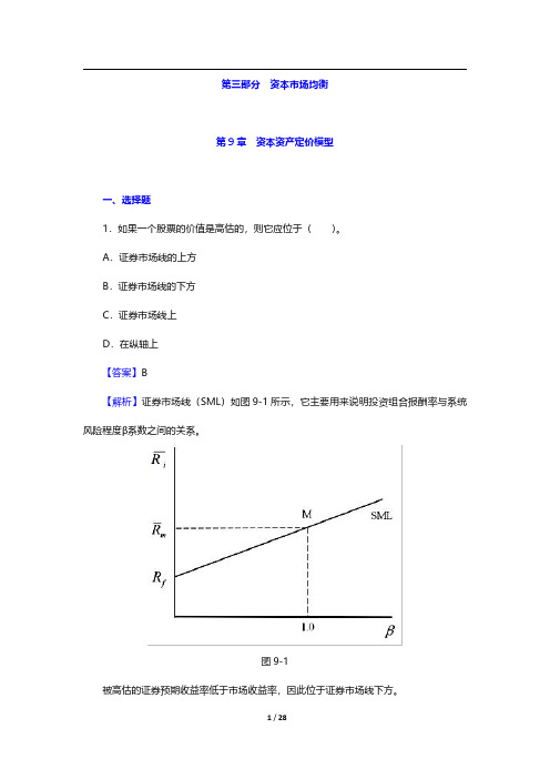
A.证券市场线的上方B.证券市场线的下方C.证券市场线上D.在纵轴上【答案】B【解析】证券市场线(SML)如图9-1所示,它主要用来说明投资组合报酬率与系统风险程度β系数之间的关系。
图9-1被高估的证券预期收益率低于市场收益率,因此位于证券市场线下方。
2.无风险利率和市场预期收益率分别是3.5%和10.5%。
根据资本资产定价模型,一只β值是1.63的证券的预期收益是()。
A.10.12%B.14.91%C.16.56%D.18.79%【答案】B【解析】根据资本资产定价模型:E(r i)=r f+β[E(r M)-r f]=3.5%+1.63×(10.5%-3.5%)=14.91%。
3.资本资产定价模型给出了精确预测()的方法。
A.有效投资组合B.单一资产与风险资产组合期望收益率C.不同风险收益偏好下最优风险投资组合D.资产风险及其期望收益率之间的关系【答案】D【解析】根据资本资产定价模型,每一证券的期望收益率应等于无风险利率加上该证券由β系数测定的风险溢价。
4.假定一只股票定价合理,预期收益是15%,市场预期收益是10.5%,无风险利率是3.5%,这只股票的β值是()。
A.1.36B.1.52C.1.64D.1.75【答案】C【解析】既然α值假定为零,证券的收益就等于CAPM设定的收益。
因此,将已知的数值代入CAPM,即15%=[3.5%+(10.5%-3.5%)β],解得:β=1.64。
5.根据CAPM模型,市场期望收益率和无风险收益率分别是0.12和0.06,β值为1.2的证券A的期望收益率是()。
A.0.068B.0.12C.0.132D.0.142【答案】C【解析】根据资本资产定价模型,E(r i)=r f+[E(r M)-r f]βi=0.06+(0.12-0.06)×1.2=0.132。
博迪《投资学》笔记和课后习题详解(最优风险资产组合)【圣才出品】

第8章最优风险资产组合8.1 复习笔记1. 分散化与资产组合风险(1)系统性风险与非系统性风险分散化能够降低风险,但是当共同的风险来源影响所有的公司时,分散化就不能消除风险了。
资产组合的标准差随着证券种类的增加而下降,但是,它不能降至零。
在最充分的分散条件下还存在着市场风险,它来源于与市场有关的因素,这种风险亦被称为“系统风险”,或“不可分散风险”。
而那些可被分散化消除的风险被称为“独特风险”、“特有公司风险”、“非系统风险”或“可分散风险”。
(2)两种风险资产的资产组合①资产组合的风险与收益资产组合的期望收益是资产组合中各种证券的期望收益的加权平均值,即:两资产的资产组合的方差是:②表格法计算组合方差表8-1显示可以通过电子表格计算资产组合的方差。
其中a表示两个共同基金收益的相邻协方差矩阵,相邻矩阵是沿着首排首列相邻每一基金在资产组合中权重的协方差矩阵。
可以通过如下方法得到资产组合的方差:斜方差矩阵中的每个因子与行、列中的权重相乘,把四个结果相加,就可以得出给出的资产组合方差。
表8-1 通过协方差矩阵计算资产组合方差③相关系数与资产组合方差具有完全正相关(相关系数为1)的资产组合的标准差恰好是资产组合中各证券标准差的加权平均值。
相关系数小于1时,资产组合的标准差小于资产组合中各证券标准差的加权平均值。
通过调整资产比例,具有完全负相关(相关系数为-1)的资产组合的标准差可以趋向0。
④资产组合比例与资产组合方差当两种资产负相关时,调整资产组合比例可以得到小于两种资产方差的最小组合方差。
若某个资产比例为负值,表示借入(或卖空)该资产。
⑤机会集机会集是指多种资产进行组合所能构成的所有风险收益的集合。
2. 资产配置(1)最优风险资产组合最优风险资产组合是使资本配置线的斜率(报酬与波动比率)最大的风险资产组合,这样表示边际风险报酬最大。
最优风险资产组合为资产配置线与机会集曲线的切点。
(2)最优完整资产组合最优完整资产组合为投资者无差异曲线与资本配置线的切点处组合,最优完整组合包含风险资产组合(债券和股票)以及无风险资产(国库券)。
Essentials Of Investments 8th Ed Bodie 投资学精要(第八版)课后习题答案Chap007
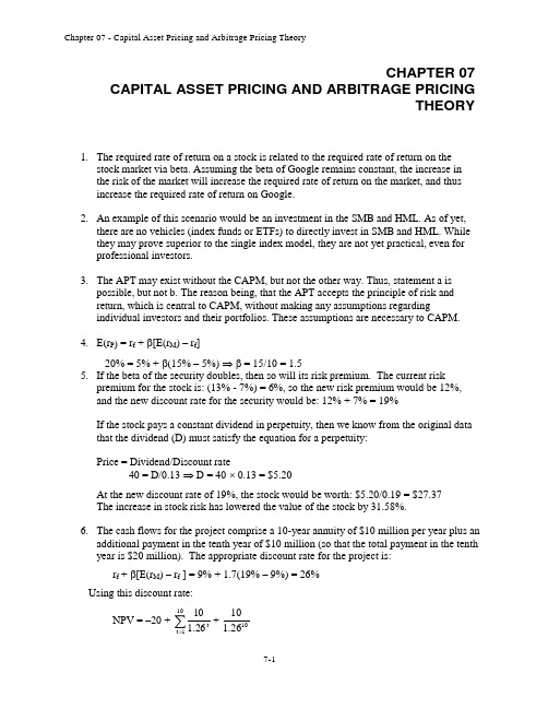
CHAPTER 07CAPITAL ASSET PRICING AND ARBITRAGE PRICINGTHEORY1. The required rate of return on a stock is related to the required rate of return on thestock market via beta. Assuming the beta of Google remains constant, the increase in the risk of the market will increase the required rate of return on the market, and thus increase the required rate of return on Google.2. An example of this scenario would be an investment in the SMB and HML. As of yet,there are no vehicles (index funds or ETFs) to directly invest in SMB and HML. While they may prove superior to the single index model, they are not yet practical, even for professional investors.3. The APT may exist without the CAPM, but not the other way. Thus, statement a ispossible, but not b. The reason being, that the APT accepts the principle of risk and return, which is central to CAPM, without making any assumptions regardingindividual investors and their portfolios. These assumptions are necessary to CAPM.4. E(r P ) = r f + β[E(r M ) – r f ]20% = 5% + β(15% – 5%) ⇒ β = 15/10 = 1.55. If the beta of the security doubles, then so will its risk premium. The current riskpremium for the stock is: (13% - 7%) = 6%, so the new risk premium would be 12%, and the new discount rate for the security would be: 12% + 7% = 19%If the stock pays a constant dividend in perpetuity, then we know from the original data that the dividend (D) must satisfy the equation for a perpetuity:Price = Dividend/Discount rate 40 = D/0.13 ⇒ D = 40 ⨯ 0.13 = $5.20 At the new discount rate of 19%, the stock would be worth: $5.20/0.19 = $27.37The increase in stock risk has lowered the value of the stock by 31.58%.6. The cash flows for the project comprise a 10-year annuity of $10 million per year plus anadditional payment in the tenth year of $10 million (so that the total payment in the tenth year is $20 million). The appropriate discount rate for the project is:r f + β[E(r M ) – r f ] = 9% + 1.7(19% – 9%) = 26% Using this discount rate:NPV = –20 + +∑=101t t26.1101026.110= –20 + [10 ⨯ Annuity factor (26%, 10 years)] + [10 ⨯ PV factor (26%, 10 years)] = 15.64The internal rate of return on the project is 49.55%. The highest value that beta can take before the hurdle rate exceeds the IRR is determined by:49.55% = 9% + β(19% – 9%) ⇒ β = 40.55/10 = 4.055 7. a. False. β = 0 implies E(r) = r f , not zero.b. False. Investors require a risk premium for bearing systematic (i.e., market orundiversifiable) risk.c. False. You should invest 0.75 of your portfolio in the market portfolio, and theremainder in T-bills. Then: βP = (0.75 ⨯ 1) + (0.25 ⨯ 0) = 0.758.a. The beta is the sensitivity of the stock's return to the market return. Call theaggressive stock A and the defensive stock D . Then beta is the change in the stock return per unit change in the market return. We compute each stock's beta by calculating the difference in its return across the two scenarios divided by the difference in market return.00.2205322A =--=β70.0205145.3D =--=βb. With the two scenarios equal likely, the expected rate of return is an average ofthe two possible outcomes: E(r A ) = 0.5 ⨯ (2% + 32%) = 17%E(r B ) = 0.5 ⨯ (3.5% + 14%) = 8.75%c. The SML is determined by the following: T-bill rate = 8% with a beta equal tozero, beta for the market is 1.0, and the expected rate of return for the market is:0.5 ⨯ (20% + 5%) = 12.5%See the following graph.812.5%S M LThe equation for the security market line is: E(r) = 8% + β(12.5% – 8%) d. The aggressive stock has a fair expected rate of return of:E(r A ) = 8% + 2.0(12.5% – 8%) = 17%The security analyst’s estimate of the expected rate of return is also 17%.Thus the alpha for the aggressive stock is zero. Similarly, the required return for the defensive stock is:E(r D ) = 8% + 0.7(12.5% – 8%) = 11.15%The security analyst’s estimate of the expected return for D is only 8.75%, and hence:αD = actual expected return – required return predicted by CAPM= 8.75% – 11.15% = –2.4%The points for each stock are plotted on the graph above.e. The hurdle rate is determined by the project beta (i.e., 0.7), not by the firm’sbeta. The correct discount rate is therefore 11.15%, the fair rate of return on stock D.9. Not possible. Portfolio A has a higher beta than Portfolio B, but the expected returnfor Portfolio A is lower.10. Possible. If the CAPM is valid, the expected rate of return compensates only forsystematic (market) risk as measured by beta, rather than the standard deviation, which includes nonsystematic risk. Thus, Portfolio A's lower expected rate of return can be paired with a higher standard deviation, as long as Portfolio A's beta is lower than that of Portfolio B.11. Not possible. The reward-to-variability ratio for Portfolio A is better than that of themarket, which is not possible according to the CAPM, since the CAPM predicts that the market portfolio is the most efficient portfolio. Using the numbers supplied:S A =5.0121016=- S M =33.0241018=-These figures imply that Portfolio A provides a better risk-reward tradeoff than the market portfolio.12. Not possible. Portfolio A clearly dominates the market portfolio. It has a lowerstandard deviation with a higher expected return.13. Not possible. Given these data, the SML is: E(r) = 10% + β(18% – 10%)A portfolio with beta of 1.5 should have an expected return of: E(r) = 10% + 1.5 ⨯ (18% – 10%) = 22%The expected return for Portfolio A is 16% so that Portfolio A plots below the SML (i.e., has an alpha of –6%), and hence is an overpriced portfolio. This is inconsistent with the CAPM.14. Not possible. The SML is the same as in Problem 12. Here, the required expectedreturn for Portfolio A is: 10% + (0.9 ⨯ 8%) = 17.2%This is still higher than 16%. Portfolio A is overpriced, with alpha equal to: –1.2%15. Possible. Portfolio A's ratio of risk premium to standard deviation is less attractivethan the market's. This situation is consistent with the CAPM. The market portfolio should provide the highest reward-to-variability ratio.16.a.b.As a first pass we note that large standard deviation of the beta estimates. None of the subperiod estimates deviate from the overall period estimate by more than two standard deviations. That is, the t-statistic of the deviation from the overall period is not significant for any of the subperiod beta estimates. Looking beyond the aforementioned observation, the differences can be attributed to different alpha values during the subperiods. The case of Toyota is most revealing: The alpha estimate for the first two years is positive and for the last two years negative (both large). Following a good performance in the "normal" years prior to the crisis, Toyota surprised investors with a negative performance, beyond what could be expected from the index. This suggests that a beta of around 0.5 is more reliable. The shift of the intercepts from positive to negative when the index moved to largely negative returns, explains why the line is steeper when estimated for the overall period. Draw a line in the positive quadrant for the index with a slope of 0.5 and positive intercept. Then draw a line with similar slope in the negative quadrant of the index with a negative intercept. You can see that a line that reconciles the observations for both quadrants will be steeper. The same logic explains part of the behavior of subperiod betas for Ford and GM.17. Since the stock's beta is equal to 1.0, its expected rate of return should be equal to thatof the market, that is, 18%. E(r) =01P P P D -+0.18 =100100P 91-+⇒ P 1 = $10918. If beta is zero, the cash flow should be discounted at the risk-free rate, 8%:PV = $1,000/0.08 = $12,500If, however, beta is actually equal to 1, the investment should yield 18%, and the price paid for the firm should be:PV = $1,000/0.18 = $5,555.56The difference ($6944.44) is the amount you will overpay if you erroneously assume that beta is zero rather than 1.ing the SML: 6% = 8% + β(18% – 8%) ⇒β = –2/10 = –0.220.r1 = 19%; r2 = 16%; β1 = 1.5; β2 = 1.0a.In order to determine which investor was a better selector of individual stockswe look at the abnormal return, which is the ex-post alpha; that is, the abnormalreturn is the difference between the actual return and that predicted by the SML.Without information about the parameters of this equation (i.e., the risk-free rateand the market rate of return) we cannot determine which investment adviser isthe better selector of individual stocks.b.If r f = 6% and r M = 14%, then (using alpha for the abnormal return):α1 = 19% – [6% + 1.5(14% – 6%)] = 19% – 18% = 1%α2 = 16% – [6% + 1.0(14% – 6%)] = 16% – 14% = 2%Here, the second investment adviser has the larger abnormal return and thusappears to be the better selector of individual stocks. By making betterpredictions, the second adviser appears to have tilted his portfolio toward under-priced stocks.c.If r f = 3% and r M = 15%, then:α1 =19% – [3% + 1.5(15% – 3%)] = 19% – 21% = –2%α2 = 16% – [3%+ 1.0(15% – 3%)] = 16% – 15% = 1%Here, not only does the second investment adviser appear to be a better stockselector, but the first adviser's selections appear valueless (or worse).21.a.Since the market portfolio, by definition, has a beta of 1.0, its expected rate ofreturn is 12%.b.β = 0 means the stock has no systematic risk. Hence, the portfolio's expectedrate of return is the risk-free rate, 4%.ing the SML, the fair rate of return for a stock with β= –0.5 is:E(r) = 4% + (–0.5)(12% – 4%) = 0.0%The expected rate of return, using the expected price and dividend for next year: E(r) = ($44/$40) – 1 = 0.10 = 10%Because the expected return exceeds the fair return, the stock must be under-priced.22.The data can be summarized as follows:ing the SML, the expected rate of return for any portfolio P is:E(r P) = r f + β[E(r M) – r f ]Substituting for portfolios A and B:E(r A) = 6% + 0.8 ⨯ (12% – 6%) = 10.8%E(r B) = 6% + 1.5 ⨯ (12% – 6%) = 15.0%Hence, Portfolio A is desirable and Portfolio B is not.b.The slope of the CAL supported by a portfolio P is given by:S =P fP σr)E(r-Computing this slope for each of the three alternative portfolios, we have:S (S&P 500) = 6/20S (A) = 5/10S (B) = 8/31Hence, portfolio A would be a good substitute for the S&P 500.23.Since the beta for Portfolio F is zero, the expected return for Portfolio F equals therisk-free rate.For Portfolio A, the ratio of risk premium to beta is: (10% - 4%)/1 = 6%The ratio for Portfolio E is higher: (9% - 4%)/(2/3) = 7.5%This implies that an arbitrage opportunity exists. For instance, you can create aPortfolio G with beta equal to 1.0 (the same as the beta for Portfolio A) by taking a long position in Portfolio E and a short position in Portfolio F (that is, borrowing at the risk-free rate and investing the proceeds in Portfolio E). For the beta of G to equal 1.0, theproportion (w) of funds invested in E must be: 3/2 = 1.5The expected return of G is then:E(r G) = [(-0.50) ⨯ 4%] + (1.5 ⨯ 9%) = 11.5%βG = 1.5 ⨯ (2/3) = 1.0Comparing Portfolio G to Portfolio A, G has the same beta and a higher expected return.Now, consider Portfolio H, which is a short position in Portfolio A with the proceedsinvested in Portfolio G:βH = 1βG + (-1)βA = (1 ⨯ 1) + [(-1) ⨯ 1] = 0E(r H) = (1 ⨯ r G) + [(-1) ⨯ r A] = (1 ⨯ 11.5%) + [(- 1) ⨯ 10%] = 1.5%The result is a zero investment portfolio (all proceeds from the short sale of Portfolio Aare invested in Portfolio G) with zero risk (because β = 0 and the portfolios are welldiversified), and a positive return of 1.5%. Portfolio H is an arbitrage portfolio.24.Substituting the portfolio returns and betas in the expected return-beta relationship, weobtain two equations in the unknowns, the risk-free rate (r f ) and the factor return (F):14.0% = r f + 1 ⨯ (F – r f )14.8% = r f + 1.1 ⨯ (F – r f )From the first equation we find that F = 14%. Substituting this value for F into the second equation, we get:14.8% = r f + 1.1 ⨯ (14% – r f ) ⇒ r f = 6%25.a.Shorting equal amounts of the 10 negative-alpha stocks and investing the proceedsequally in the 10 positive-alpha stocks eliminates the market exposure and creates azero-investment portfolio. Using equation 7.5, and denoting the market factor as R M,the expected dollar return is [noting that the expectation of residual risk (e) inequation 7.8 is zero]:$1,000,000 ⨯ [0.03 + (1.0 ⨯ R M)] – $1,000,000 ⨯ [(–0.03) + (1.0 ⨯ R M)]= $1,000,000 ⨯ 0.06 = $60,000The sensitivity of the payoff of this portfolio to the market factor is zero because theexposures of the positive alpha and negative alpha stocks cancel out. (Notice thatthe terms involving R M sum to zero.) Thus, the systematic component of total riskalso is zero. The variance of the analyst's profit is not zero, however, since thisportfolio is not well diversified.For n = 20 stocks (i.e., long 10 stocks and short 10 stocks) the investor will have a$100,000 position (either long or short) in each stock. Net market exposure is zero,but firm-specific risk has not been fully diversified. The variance of dollar returnsfrom the positions in the 20 firms is:20 ⨯ [(100,000 ⨯ 0.30)2] = 18,000,000,000The standard deviation of dollar returns is $134,164.b.If n = 50 stocks (i.e., 25 long and 25 short), $40,000 is placed in each position,and the variance of dollar returns is:50 ⨯ [(40,000 ⨯ 0.30)2] = 7,200,000,000The standard deviation of dollar returns is $84,853.Similarly, if n = 100 stocks (i.e., 50 long and 50 short), $20,000 is placed ineach position, and the variance of dollar returns is:100 ⨯ [(20,000 ⨯ 0.30)2] = 3,600,000,000The standard deviation of dollar returns is $60,000.Notice that when the number of stocks increases by a factor of 5 (from 20 to 100),standard deviation falls by a factor of 5= 2.236, from $134,164 to $60,000. 26.Any pattern of returns can be "explained" if we are free to choose an indefinitely largenumber of explanatory factors. If a theory of asset pricing is to have value, it mustexplain returns using a reasonably limited number of explanatory variables (i.e.,systematic factors).27.The APT factors must correlate with major sources of uncertainty, i.e., sources ofuncertainty that are of concern to many investors. Researchers should investigatefactors that correlate with uncertainty in consumption and investment opportunities.GDP, the inflation rate and interest rates are among the factors that can be expected to determine risk premiums. In particular, industrial production (IP) is a good indicator of changes in the business cycle. Thus, IP is a candidate for a factor that is highlycorrelated with uncertainties related to investment and consumption opportunities in the economy.28.The revised estimate of the expected rate of return of the stock would be the oldestimate plus the sum of the unexpected changes in the factors times the sensitivitycoefficients, as follows:Revised estimate = 14% + [(1 ⨯ 1) + (0.4 ⨯ 1)] = 15.4%29.Equation 7.11 applies here:E(r P) = r f + βP1[E(r1) - r f] + βP2[E(r2) – r f]We need to find the risk premium for these two factors:γ1 = [E(r1) - r f] andγ2 = [E(r2) - r f]To find these values, we solve the following two equations with two unknowns: 40% = 7% + 1.8γ1 + 2.1γ210% = 7% + 2.0γ1 + (-0.5)γ2The solutions are: γ1 = 4.47% and γ2 = 11.86%Thus, the expected return-beta relationship is:E(r P) = 7% + 4.47βP1 + 11.86βP230.The first two factors (the return on a broad-based index and the level of interest rates)are most promising with respect to the likely impa ct on Jennifer’s firm’s cost of capital.These are both macro factors (as opposed to firm-specific factors) that can not bediversified away; consequently, we would expect that there is a risk premiumassociated with these factors. On the other hand, the risk of changes in the price ofhogs, while important to some firms and industries, is likely to be diversifiable, andtherefore is not a promising factor in terms of its impact on the firm’s cost of capital.31.Since the risk free rate is not given, we assume a risk free rate of 0%. The APT required(i.e., equilibrium) rate of return on the stock based on Rf and the factor betas is:Required E(r) = 0 + (1 x 6) + (0.5 x 2) + (0.75 x 4) = 10%According to the equation for the return on the stock, the actually expected return onthe stock is 6 % (because the expected surprises on all factors are zero by definition).Because the actually expected return based on risk is less than the equilibrium return,we conclude that the stock is overpriced.CFA 1a, c and dCFA 2a.E(r X) = 5% + 0.8(14% – 5%) = 12.2%αX = 14% – 12.2% = 1.8%E(r Y) = 5% + 1.5(14% – 5%) = 18.5%αY = 17% – 18.5% = –1.5%b.(i)For an investor who wants to add this stock to a well-diversified equityportfolio, Kay should recommend Stock X because of its positivealpha, while Stock Y has a negative alpha. In graphical terms, StockX’s expected return/risk profile plots above the SML, while Stock Y’sprofile plots below the SML. Also, depending on the individual riskpreferences of Kay’s clients, Stock X’s lower beta may have abeneficial impact on overall portfolio risk.(ii)For an investor who wants to hold this stock as a single-stock portfolio,Kay should recommend Stock Y, because it has higher forecastedreturn and lower standard deviation than S tock X. Stock Y’s Sharperatio is:(0.17 – 0.05)/0.25 = 0.48Stock X’s Sharpe ratio is only:(0.14 – 0.05)/0.36 = 0.25The market index has an even more attractive Sharpe ratio:(0.14 – 0.05)/0.15 = 0.60However, given the choice between Stock X and Y, Y is superior.When a stock is held in isolation, standard deviation is the relevantrisk measure. For assets held in isolation, beta as a measure of risk isirrelevant. Although holding a single asset in isolation is not typicallya recommended investment strategy, some investors may hold what isessentially a single-asset portfolio (e.g., the stock of their employercompany). For such investors, the relevance of standard deviationversus beta is an important issue.CFA 3a.McKay should borrow funds and i nvest those funds proportionally in Murray’sexisting portfolio (i.e., buy more risky assets on margin). In addition toincreased expected return, the alternative portfolio on the capital market line(CML) will also have increased variability (risk), which is caused by the higherproportion of risky assets in the total portfolio.b.McKay should substitute low beta stocks for high beta stocks in order to reducethe overall beta of York’s portfolio. By reducing the overall portfolio beta,McKay will reduce the systematic risk of the portfolio and therefore theportfolio’s volatility relative to the market. The security market line (SML)suggests such action (moving down the SML), even though reducing beta mayresult in a slight loss of portfolio efficiency unless full diversification ismaintained. York’s primary objective, however, is not to maintain efficiencybut to reduce risk exposure; reducing portfolio beta meets that objective.Because York does not permit borrowing or lending, McKay cannot reduce riskby selling equities and using the proceeds to buy risk free assets (i.e., by lendingpart of the portfolio).CFA 4c.“Both the CAPM and APT require a mean-variance efficient market portfolio.”This statement is incorrect. The CAPM requires the mean-variance efficientportfolio, but APT does not.d.“The CAPM assumes that one specific factor explains security returns but APTdoes not.” This statement is c orrect.CFA 5aCFA 6dCFA 7d You need to know the risk-free rate.CFA 8d You need to know the risk-free rate.CFA 9Under the CAPM, the only risk that investors are compensated for bearing is the riskthat cannot be diversified away (i.e., systematic risk). Because systematic risk(measured by beta) is equal to 1.0 for each of the two portfolios, an investor wouldexpect the same rate of return from each portfolio. Moreover, since both portfolios are well diversified, it does not matter whether the specific risk of the individual securities is high or low. The firm-specific risk has been diversified away from both portfolios. CFA 10b r f = 8% and E(r M) = 16%E(r X) = r f + βX[E(r M) – r f] = 8% + 1.0(16% - 8%) = 16%E(r Y) = r f + βY[E(r M) – r f] = 8% + 0.25(16% - 8%) = 10%Therefore, there is an arbitrage opportunity.CFA 11cCFA 12dCFA 13cInvestors will take on as large a position as possible only if the mis-pricingopportunity is an arbitrage. Otherwise, considerations of risk anddiversification will limit the position they attempt to take in the mis-pricedsecurity.CFA 14d。
投资学第10章习题及答案

第10章习题及答案1.2008年金融危机对我国股市有何影响?2.货币政策如何影响股市的?3.2008年以来我国实施的宽松的财政政策对于股票市场有何影响?4.简述经济周期与证券市场波动之间的关系?5.影响行业兴衰的因素都有哪些?6.一个公司的行业敏感性取决于哪些因素?参考答案1.国际经济关系对证券市场的影响,包括国际经济的增长状况、国际金融以及利率与汇率的变动、境外股市行情波动、贸易关系等。
其中国际金融以及利率与汇率的变动对于证券市场的影响非常大。
西方主要国际金融市场的利率一旦发生变化,证券市场也会相应的发生变化,即利率的提高将会带来证券市场的下跌趋势,反之利率的降低,证券市场就会上涨。
境外股市行情的波动会立刻影响到我国股市的波动。
一国因为某种因素引发股市危机,就会引发连锁的股市灾难。
另外,贸易关系的改变通常会引起相关国际性公司股票价格发生波动。
如果一国贸易对国际市场依赖性比较大,那么,贸易关系的改善,将会推动该国股市指数的大幅上涨;相反,如果贸易关系恶化,通常会引起该国股市指数的大幅下挫。
例如07年爆发美国次贷危机中,美国股市下跌了55%,以此同时,受到牵连的中国股市跌幅达到73%。
2.从证券投资的角度看, 货币政策可以直接影响证券市场行情。
中央银行的货币政策对证券的价格有重要影响。
从整体来说, 宽松的货币政策将会使证券市场价格上涨;而从紧的货币政策将会使证券市场价格下跌。
货币政策对证券市场的影响可以从四个方面来分析: (1)利率政策对于证券市场价格具有重要影响。
通常证券价格对利率的变动较为敏感。
(2)中央银行的微调政策对证券价格的影响具体表现如下:如果放松银根, 中央银行将大量买进证券, 增加了社会对证券的需求, 引起证券价格上升;如果紧缩银根,中央银行将抛出证券, 使证券供给过旺, 导致价格下跌。
(3)货币政策的综合影响, 当货币供应量过多而造成通货膨胀时, 人们为保值而购买证券(尤其是股票) , 推动证券需求上升, 价格上涨; 当货币供应量不足时, 人们为取得货币资金而抛售证券, 使证券价格下跌。
投资学 (博迪) 第10版课后习题答案19 Investments 10th Edition Textbook Solutions Chapter 19
15. a. The total capital of the firms must first be calculated by adding their respective debt and equity together. The total capital for Acme is 100 + 50 = 150, and the total capital for Apex is 450 + 150 = 600. The economic value added will be the spread between the ROC and cost of capital multiplied by the total capital of the firm. Acme’s EVA thus equals (17% − 9%) × 150 = 12 (million). Apex’s EVA equals (15% − 10%) × 600 = 30 (mil). Notice that even though Apex’s spread is smaller, their larger capital stock allows them more economic value added.
Alternatively, 0.03 = 0.65 × [ROA + (ROA - 0.06) × 0.5] 0.0462 = [ROA + (ROA - 0.06) × 0.5] 0.0462 = ROA + 0.5ROA - 0.03 0.0762 = ROA + 0.5ROA 0.0762 = 1.5ROA 0.0508 = ROA
2. Earnings management should not matter in a truly efficient market, where all publicly available information is reflected in the price of a share of stock. Investors can see through attempts to manage earnings so that they can determine a company’s true profitability and, hence, the intrinsic value of a share of stock. However, if firms do engage in earnings management, then the clear implication is that managers do not view financial markets as efficient.
- 1、下载文档前请自行甄别文档内容的完整性,平台不提供额外的编辑、内容补充、找答案等附加服务。
- 2、"仅部分预览"的文档,不可在线预览部分如存在完整性等问题,可反馈申请退款(可完整预览的文档不适用该条件!)。
- 3、如文档侵犯您的权益,请联系客服反馈,我们会尽快为您处理(人工客服工作时间:9:00-18:30)。
CHAPTER 10: ARBITRAGE PRICING THEORYAND MULTIFACTOR MODELS OF RISK AND RETURNPROBLEM SETS1. The revised estimate of the expected rate of return on the stock wouldbe the old estimate plus the sum of the products of the unexpectedchange in each factor times the respective sensitivity coefficient: revised estimate = 12% + [(1 2%) + (0.5 3%)] = 15.5%2. The APT factors must correlate with major sources of uncertainty, i.e.,sources of uncertainty that are of concern to many investors.Researchers should investigate factors that correlate with uncertaintyin consumption and investment opportunities. GDP, the inflation rate,and interest rates are among the factors that can be expected todetermine risk premiums. In particular, industrial production (IP) is a good indicator of changes in the business cycle. Thus, IP is acandidate for a factor that is highly correlated with uncertaintiesthat have to do with investment and consumption opportunities in theeconomy.3. Any pattern of returns can be “explained” if we are free to choose anindefinitely large number of explanatory factors. If a theory of assetpricing is to have value, it must explain returns using a reasonablylimited number of explanatory variables (i.e., systematic factors).4. Equation 10.9 applies here:E(r p) = r f + P1 [E(r1 ) r f ] + P2 [E(r2) – r f ]We need to find the risk premium (RP) for each of the two factors: RP1 = [E(r1) r f ] and RP2 = [E(r2) r f ]In order to do so, we solve the following system of two equations with two unknowns:31 = 6 + (1.5 RP1) + (2.0 RP2)27 = 6 + (2.2 RP1) + [(–0.2) RP2]The solution to this set of equations is:RP1 = 10% and RP2 = 5%Thus, the expected return-beta relationship is: E(r P) = 6% + (P1 10%) + (P2 5%)5. The expected return for Portfolio F equals the risk-free rate since itsbeta equals 0.For Portfolio A, the ratio of risk premium to beta is: (12 6)/1.2 = 5For Portfolio E, the ratio is lower at: (8 – 6)/0.6 = 3.33This implies that an arbitrage opportunity exists. For instance, youcan create a Portfolio G with beta equal to 0.6 (the same as E’s) by combining Portfolio A and Portfolio F in equal weights. The expectedreturn and beta for Portfolio G are then:E(r G ) = (0.5 12%) + (0.5 6%) = 9%G = (0.5 1.2) + (0.5 0) = 0.6Comparing Portfolio G to Portfolio E, G has the same beta and higherreturn. Therefore, an arbitrage opportunity exists by buying PortfolioG and selling an equal amount of Portfolio E. The profit for thisarbitrage will be:r G– r E =[9% + (0.6 F)] [8% + (0.6 F)] = 1%That is, 1% of the funds (long or short) in each portfolio.6. Substituting the portfolio returns and betas in the expected return-beta relationship, we obtain two equations with two unknowns, the risk-free rate (r f ) and the factor risk premium (RP):12 = r f + (1.2 RP)9 = r f + (0.8 RP)Solving these equations, we obtain:r f = 3% and RP = 7.5%7. a. Shorting an equally-weighted portfolio of the ten negative-alphastocks and investing the proceeds in an equally-weighted portfolioof the ten positive-alpha stocks eliminates the market exposure andcreates a zero-investment portfolio. Denoting the systematic marketfactor as R M , the expected dollar return is (noting that theexpectation of non-systematic risk, e, is zero):$1,000,000 [0.02 + (1.0 R M )] $1,000,000 [(–0.02)+ (1.0 R M )]= $1,000,000 0.04 = $40,000The sensitivity of the payoff of this portfolio to the market factor is zero because the exposures of the positive alpha and negative alpha stocks cancel out. (Notice that the terms involving R M sum to zero.) Thus, the systematic component of total risk is also zero. The variance of the analyst’s profit is not zero, however, since this portfolio is not well diversified.For n = 20 stocks (i.e., long 10 stocks and short 10 stocks) the investor will have a $100,000 position (either long or short) in each stock. Net market exposure is zero, but firm-specific risk has not been fully diversified. The variance of dollar returns from the positions in the 20 stocks is: 20 [(100,000 0.30)2 ] = 18,000,000,000 The standard deviation of dollar returns is $134,164.b.If n = 50 stocks (25 stocks long and 25 stocks short), the investor will have a $40,000 position in each stock, and the variance of dollar returns is: 50 [(40,000 0.30)2 ] = 7,200,000,000 The standard deviation of dollar returns is $84,853. Similarly, if n = 100 stocks (50 stocks long and 50 stocks short), the investor will have a $20,000 position in each stock, and the variance of dollar returns is: 100 [(20,000 0.30)2 ] = 3,600,000,000 The standard deviation of dollar returns is $60,000. Notice that, when the number of stocks increases by a factor of 5 (i.e., from 20 to 100), standard deviation decreases by a factor of 5= 2.23607 (from $134,164 to $60,000).8. a.)e (22M 22σ+σβ=σ 88125)208.0(2222A =+⨯=σ 50010)200.1(2222B =+⨯=σ 97620)202.1(2222C =+⨯=σb.If there are an infinite number of assets with identical characteristics, then a well-diversified portfolio of each type will have only systematic risk since the non-systematic risk will approach zero with large n. The mean will equal that of the individual (identical) stocks.c. There is no arbitrage opportunity because the well-diversifiedportfolios all plot on the security market line (SML). Becausethey are fairly priced, there is no arbitrage.9. a. A long position in a portfolio (P) comprised of Portfolios A and Bwill offer an expected return-beta tradeoff lying on a straightline between points A and B. Therefore, we can choose weights suchthat P = C but with expected return higher than that ofPortfolio C. Hence, combining P with a short position in C willcreate an arbitrage portfolio with zero investment, zero beta, andpositive rate of return.b. The argument in part (a) leads to the proposition that thecoefficient of 2 must be zero in order to preclude arbitrageopportunities.10. a. E(r) = 6 + (1.2 6) + (0.5 8) + (0.3 3) = 18.1%b.Surprises in the macroeconomic factors will result in surprises inthe return of the stock:Unexpected return from macro factors =[1.2(4 – 5)] + [0.5(6 – 3)] + [0.3(0 – 2)] = –0.3%E (r) =18.1% − 0.3% = 17.8%11. The APT required (i.e., equilibrium) rate of return on the stock basedon r f and the factor betas is:required E(r) = 6 + (1 6) + (0.5 2) + (0.75 4) = 16%According to the equation for the return on the stock, the actuallyexpected return on the stock is 15% (because the expected surprises on all factors are zero by definition). Because the actually expectedreturn based on risk is less than the equilibrium return, we conclude that the stock is overpriced.12. The first two factors seem promising with respect to the likely impacton the firm’s cost of capital. Both are macro factors that would elicit hedging demands across broad sectors of investors. The third factor,while important to Pork Products, is a poor choice for a multifactor SML because the price of hogs is of minor importance to most investors and is therefore highly unlikely to be a priced risk factor. Better choices would focus on variables that investors in aggregate might find moreimportant to their welfare. Examples include: inflation uncertainty,short-term interest-rate risk, energy price risk, or exchange rate risk.The important point here is that, in specifying a multifactor SML, we not confuse risk factors that are important to a particular investorwith factors that are important to investors in general; only the latter are likely to command a risk premium in the capital markets.13. The maximum residual variance is tied to the number of securities (n)in the portfolio because, as we increase the number of securities, weare more likely to encounter securities with larger residual variances.The starting point is to determine the practical limit on the portfolio residual standard deviation, (e P), that still qualifies as a ‘well-diversified portfolio.’ A reasonable approach is to compare 2(e P) to the market variance, or equivalently, to compare (e P) to the marketstandard deviation. Suppose we do not allow (e P) to exceed p M, where p is a small decimal fraction, for example, 0.05; then, the smaller the value we choose for p, the more stringent our criterion for defininghow diversified a ‘well-diversified’ portfolio must be.Now construct a portfolio of n securities with weights w1, w2,…,w n, sothat w i =1. The portfolio residual variance is: 2(e P) = w122(e i)To meet our practical definition of sufficiently diversified, werequire this residual variance to be less than (p M)2. A sure andsimple way to proceed is to assume the worst, that is, assume that the residual variance of each security is the highest possible valueallowed under the assumptions of the problem: 2(e i) = n2MIn that case: 2(e P) = w i2n M2Now apply the constraint: w i2 n M2 ≤ (p M)2This requires that: n w i2≤ p2Or, equivalently, that: w i2 ≤ p2/nA relatively easy way to generate a set of well-diversified portfolios isto use portfolio weights that follow a geometric progression, since the computations then become relatively straightforward. Choose w1 and acommon factor q for the geometric progression such that q < 1. Therefore, the weight on each stock is a fraction q of the weight on the previous stock in the series. Then the sum of n terms is:w i= w1(1– q n)/(1– q) = 1or: w1 = (1– q)/(1–q n)The sum of the n squared weights is similarly obtained from w12 and acommon geometric progression factor of q2. Therefore:w i2 = w12(1– q2n)/(1– q 2)Substituting for w1 from above, we obtain:w i2 = [(1– q)2/(1–q n)2] × [(1– q2n)/(1– q 2)]For sufficient diversification, we choose q so that: w i2 ≤ p2/nFor example, continue to assume that p = 0.05 and n = 1,000. If wechooseq = 0.9973, then we will satisfy the required condition. At this valuefor q:w1 = 0.0029 and w n = 0.0029 × 0.99731,000In this case, w1 is about 15 times w n. Despite this significantdeparture from equal weighting, this portfolio is nevertheless welldiversified. Any value of q between 0.9973 and 1.0 results in a well-diversified portfolio. As q gets closer to 1, the portfolio approachesequal weighting.14. a. Assume a single-factor economy, with a factor risk premium E M and a(large) set of well-diversified portfolios with beta P. Supposewe create a portfolio Z by allocating the portion w to portfolio Pand (1 – w) to the market portfolio M. The rate of return onportfolio Z is:R Z = (w × R P) + [(1 – w) × R M]Portfolio Z is riskless if we choose w so that Z = 0. Thisrequires that:Z = (w × P) + [(1 – w) × 1] = 0 w = 1/(1 –P) and (1 – w) = –P/(1 –P)Substitute this value for w in the expression for R Z:R Z = {[1/(1 –P)] × R P} – {[P/(1 –P)] × R M}Since Z = 0, then, in order to avoid arbitrage, R Z must be zero.This implies that: R P = P× R MTaking expectations we have:E P = P× E MThis is the SML for well-diversified portfolios.b. The same argument can be used to show that, in a three-factormodel with factor risk premiums E M, E1 and E2, in order to avoidarbitrage, we must have:E P = (PM× E M) + (P1× E1) + (P2× E2)This is the SML for a three-factor economy.15. a. The Fama-French (FF) three-factor model holds that one of thefactors driving returns is firm size. An index with returns highlycorrelated with firm size (i.e., firm capitalization) thatcaptures this factor is SMB (Small Minus Big), the return for aportfolio of small stocks in excess of the return for a portfolioof large stocks. The returns for a small firm will be positivelycorrelated with SMB. Moreover, the smaller the firm, the greaterits residual from the other two factors, the market portfolio andthe HML portfolio, which is the return for a portfolio of highbook-to-market stocks in excess of the return for a portfolio oflow book-to-market stocks. Hence, the ratio of the variance ofthis residual to the variance of the return on SMB will be largerand, together with the higher correlation, results in a high betaon the SMB factor.b.This question appears to point to a flaw in the FF model. Themodel predicts that firm size affects average returns, so that, iftwo firms merge into a larger firm, then the FF model predictslower average returns for the merged firm. However, there seems tobe no reason for the merged firm to underperform the returns ofthe component companies, assuming that the component firms wereunrelated and that they will now be operated independently. Wemight therefore expect that the performance of the merged firmwould be the same as the performance of a portfolio of theoriginally independent firms, but the FF model predicts that theincreased firm size will result in lower average returns.Therefore, the question revolves around the behavior of returnsfor a portfolio of small firms, compared to the return for largerfirms that result from merging those small firms into larger ones.Had past mergers of small firms into larger firms resulted, onaverage, in no change in the resultant larger firms’ stock returncharacteristics (compared to the portfolio of stocks of the mergedfirms), the size factor in the FF model would have failed.Perhaps the reason the size factor seems to help explain stock returns is that, when small firms become large, thecharacteristics of their fortunes (and hence their stock returns) change in a significant way. Put differently, stocks of large firms that result from a merger of smaller firms appearempirically to behave differently from portfolios of the smaller component firms. Specifically, the FF model predicts that the large firm will have a smaller risk premium. Notice that this development is not necessarily a bad thing for the stockholders of the smaller firms that merge. The lower risk premium may be due, in part, to the increase in value of the larger firm relative to the merged firms.CFA PROBLEMS1. a. This statement is incorrect. The CAPM requires a mean-varianceefficient market portfolio, but APT does not.b.This statement is incorrect. The CAPM assumes normally distributedsecurity returns, but APT does not.c. This statement is correct.2. b. Since Portfolio X has = 1.0, then X is the market portfolio andE(R M) =16%. Using E(R M ) = 16% and r f = 8%, the expected return forportfolio Y is not consistent.3. d.4. c.5. d.6. c. Investors will take on as large a position as possible only if themispricing opportunity is an arbitrage. Otherwise, considerationsof risk and diversification will limit the position they attemptto take in the mispriced security.7. d.8. d..。