Two-level system with a thermally fluctuating transfer matrix element Application to the pr
PEROXCAP 氢氧化酸浓度传感器说明书

Measurement conditions Q: Does the probewithstand condensation?A: Yes. When powered on, the PEROXCAP ® sensor is heated, which permits use in condensing VH 2O 2 conditions. The heating maintains measurementperformance and lengthens the probe’s lifetime. The probe must always be powered on with H 2O 2 present. Exposing the probe to H 2O 2 condensation is notrecommended with the power off.Q: Can the probe measure liquid H 2O 2?A: No, the HPP270 probe isdesigned to measure vaporized hydrogen peroxide only.Q: Can the probe be used in vacuum conditions?A: The probe is not designed to be used under vacuum conditions. Vacuum conditions will cause the measurement to drift and could harm the humidity sensors.Q: Can I use this probe in over / under pressure?A: The HPP270 probe is designed for normal atmospheric pressure only. While the probe can withstand slight over/under pressure, pressure influences the ppm calculation. The probe does not have on-board pressure measurement, but a pressure reading from an external source can be used as a setpoint value for limited range compensation. You can configure the pressure compensation parameters using Vaisala Insight software, Modbus configuration registers, or an Indigo 200 or 500 transmitter.Q: What happens if the probe reads above 2000 ppm?A: The HPP272 probe withstands concentrations greater than 2000 ppm but higher H 2O 2 concentrations will negatively impact the probe’s lifespan and increase sensor drift.Q: What are theacceptable flow rates for the probes?A: The white filter on theprobe covers the PEROXCAP ® sensor. This porous PTFE filter allows ambient air to reach the PEROXCAP ® sensor while protecting the sensor. We have tested different airflows for RH measurement only, but do not predict any negative effect on the H 2O 2 ppm readings.HPP270 Series probes for vaporized hydrogen peroxide measurement: Frequently Asked QuestionsThe Vaisala PEROXCAP® HPP270 series probes (HPP271 and HPP272) are designed for demanding vaporized hydrogenperoxide bio-decontamination applications. The probes provide repeatable, stable, and accurate measurements and are ideal for VH 2O 2 bio-decontamination in environments such as isolators, material transfer hatches, and rooms. In this technical note we answer common questions on the HPP270 series vaporized hydrogen peroxide probes.FAQsMeasurementQ: What benefit does Vaisala traceable factory calibration bring to the HPP270-series probes?A: Traceability: a traceable measurement can be linkedto appropriate national or international standards through a documented, unbrokenchain of comparisons. Vaisala’s calibration laboratory has aworld-class H2O2vapor calibrationstation. The calibration station’sH2O2ppm value can be tracedto international standards. This means that we can rely on the ppm concentration value it generates.Q: How are relative humidity and relative saturation measured by the HPP270-series probes?A: The PEROXCAP® sensor contains two differentHUMICAP® sensors: A standard HUMICAPR2 and a HUMICAPR2 with a catalytic layer. The catalytic layer on one of the humiditysensors decomposes the H2O2vapor into water and oxygen. Thisprevents any H2O2measurementby one of the HUMICAP® sensors. Relative saturation is a calculated value based on the different measurements from the two humidity sensors, one with and one without a catalytic layer. Calculated RS% is derived from the different relative humidity, ppm and temperature measurements of both sensors.Q: What is the lowestppm that the probe canmeasure?A: The measurement scale is from0 to 2000 ppm with the accuracyof 10 ppm or 5% of the reading(whichever is greater) at 25 °C.The accuracy specifications arestated from 10 ppm onwards. TheHPP270 series probes are notdesigned for low level or sub-ppmlevel measurements.Q: Why is the absolutehydrogen peroxide unitmg/m3 and not mg/L?What is the conversion?A: We have chosen to usemg/m3 because it is an SI unit,and mg/L is not. AbsoluteH2O2mg/m3 (milligrams per cubicmeter) can be converted into mg/L(milligrams per liter) by using thisformula:(H2O2) = M H2O2∙ P ∙ H2O2ppm / TWhere:M H2O2= Molecular mass of H2O2P = PressureH2O2ppm = Measured H2O2concentration in ppmvT = Measured temperatureQ: Why does the HPP271only output ppm, butnot relative humidity andrelative saturation?A: The HPP271 probe containsa PEROXCAP® sensor that iswarmed in order to provide stable,accurate and repeatable VH2O2measurement in condensingenvironments.The HPP272 probe can providevalues for relative humidityand relative saturation becauseit comes with an additionaltemperature sensor. Relativehumidity and relative saturationare temperature-dependentparameters. The HPP271 doesnot have this required additionaltemperature sensor and thereforecan only measure H2O2ppm.With the temperature probe, theHPP272 probe can output ppm,%RH and %RS.Q: Why does the analogppm output not alwaysgo to zero with no H2O2present?A: The PEROXCAP® sensorconsists of two humidity sensorsthat have a minor differencein behavior when the humiditylevel changes. Because of thisdifference, the H2O2concentrationreading may vary slightly (typically0 … 3ppm) even when the probe isnot exposed to H2O2.If necessary, the variation in low level output can be hidden byenabling the low H2O2thresholdfeature that forces the output to 0 when the measurement falls below a set level (for example, 3 ppm), and the configured activation delay ends.The output returns to normal operation after the measurement has remained above the set deactivation level (for example,10 ppm) for a set time. You canconfigure the low H2O2 thresholdactivation and deactivation levels and the activation and deactivation delays with Vaisala Insight PC software and Modbus registers.Q: What kind of heating functions do the sensors have?A: When powered on, the PEROXCAP® sensor is heated. This prevents condensationfrom forming on the sensor and provides reliable measurement even in condensing environments. Heating also helps to maintain measurement performance and lengthens the probe’s lifetime.In addition, the probes feature a chemical purge cycle that heats the sensor at certain intervals. The chemical purge causes the rapid evaporation of chemical contaminants that may have been absorbed by the polymer. This chemical purge feature cleans the sensor internally, maintaining its stability and accuracy.Chemical purgeQ: When does thechemical purge cycleoccur?A: The purge cycle is initiated inthree ways:• Automatically when the probe ispowered on.• When manually triggered, whichthen re-sets the purge interval.• At regular intervals (the defaultpurge cycle is every 24 hours,but purge cycles are configurablebetween one hour and one weekusing Vaisala’s Insight software,Modbus, or Indigo 200 and 500transmitters.Q: How can I ensure thechemical purge doesn’toccur during the bio-decontamination cycle?A: The chemical purge isautomatically performed atintervals, however, the purgecycle is postponed by 30 minutesif H2O2is present or the relativehumidity has not stabilized.The purge cycle is essential forthe accuracy and long-termperformance of the probe indemanding H2O2environments.During a purge cycle,H2O2and H2O measurements arenot available.Q: How often is thechemical purgerecommended?A chemical purge is recommendedat least every 24 hours ofpowered-on time, even if theprobe has not been continuouslyexposed to H2O2. If triggeredpurge is used, we recommendimplementing the purge prior to abio-decontamination. Note, that ittakes approximately nine minutesto get accurate results after apurge. Increased exposure to H2O2will warrant more frequent purges.The maximum purge interval isonce a week.Calibration andmaintenanceQ: Can a user replace thePEROXCAP® sensors?A: No, you cannot replace thesensors. They are not soldseparately and a factory-levelcalibration and adjustment needsto be performed after a sensorreplacement. This ensures themeasurement performance of thePEROXCAP® probe.Q: Can I replace the filterby myself? Can I orderthe filter as a spare part?A: Yes, you can replace thefilter. The part number isDRW246363SP.Q: Can I do an on-site calibration and adjustment?A: Yes, the HPP270 series probes can be calibrated in the field in a couple of ways.Because the PEROXCAP® sensor is composed of two HUMICAP®humidity sensors with theH2O2measurement based oncalculations from both sensors, a field calibration and adjustment can be performed using a humidity standard reference, such asour HMK15 Humidity Calibrator. Vaisala’s Insight software is required for calibration and adjustment. Additional details for this procedure can be found in the HPP270 series probe User Guide. Another option is a calibration using a recently calibrated HPP270 series probe. With the calibratedH2O2measurement, calibrationsand adjustments can be made through the Insight PC Software, or with an Indigo transmitter. These calibrations are difficult due to the challenge of producinga stable H2O2environment. It isrecommended that this type of calibration be performed by one of Vaisala’s calibration labs.Q: How do you know if the catalytic layer is still ok?A: We have performed extensive, long-term testing on the catalyticlayer in a vaporized H2O2environment. These tests indicate that the catalytic layer is durable. You can spot-check the catalyticlayer by comparing the H2O2ppmvalues to those of a calibrated andadjusted HPP270 series probe.Q: How often do I need tocalibrate the probe?A: The HPP270 series probes donot have a specified calibrationinterval. The typical calibrationinterval is one year, however theneed for calibration is based uponthe duration and concentrationof H2O2exposure and thereqirements of your internalquality management system. TheVaisala Insight software allowsyou to perform sensor diagnosticsand view information on sensorfunction, called “Sensor Vitality”.Sensor vitality is displayed asa percentage. We recommendreplacing HPP270 series probeswhen the sensor vitality valuereaches ≤40%.Q: What does the SensorVitality percentagemean?A: Due to the stresses ofthe VH2O2environment, thePEROXCAP® sensor will losesome functionality over time. Inless demanding conditions, thesensor can remain functionalfor many years. In environmentswith higher H2O2concentrationsand longer exposure periods, itis recommended to monitor thecondition of the sensor regularly.Within the Vaisala Insight software,the status of the sensor can beviewed in Diagnostics Data.>Devices > [probe name] >Diagnostics. In the DiagnosticsData view, the condition of thesensor is shown as a percentage(0 … 100 %) on the SensorVitality row. A new sensor willhave a sensor vitality of 100 %and a sensor at the end of its lifecycle will have a sensor vitalityof 0 %. If you are using the probein a demanding environment,contact Vaisala to arrange sensorreplacement once the sensorvitality value reaches 40 %.Q: Can I customize theoutput (measurementscale)?A: Yes, the analog output scalecan be customized for all of theavailable parameters. This canbe performed using the Insightsoftware, Modbus registers, orthrough the Indigo 200 and 500configuration interface.Q: Can changes to theprobe be made in thefield?A: Yes, you can change the outputparameters, output scaling, andchemical purge intervals. Makethese changes using Vaisala’sInsight software, Modbus registers,or through the Indigo transmitter’sconfiguration interface.INDIGO 200 & 500 seriestransmittersQ: Are the HPP271 and HPP272 probes compatible with Indigo 200 and 500 Series?A: Yes, connecting the probe to an Indigo transmitter provides a range of additional options for outputs, measurementviewing, status monitoring, and configuration.Additional features with Indigo transmitters: Indigo 200 Series• 3.5” LCD color display or non-display model with LED indicator • Digital output or 3 analog outputs (depending on the transmitter model)• 2 configurable relays• Wireless browser-basedconfiguration interface for mobile devices and computers (IEEE 802.11 b/g/n WLAN)Indigo 500 Series • Dual probe support • T ouchscreen display• Digital output or 4 configurable analog outputs and 2 configurable relays • Power over Ethernet optionQ: Can the purge function of the HPP272 betriggered by the Indigo?A: Yes, you can trigger and modify the purge function by using the Indigo 200 and 500 transmitters.Learn more at/hpp270Please contact us at/contactusScan the code formore informationRef. B212113EN-A ©Vaisala 2020This material is subject to copyright protection, with all copyrights retained by Vaisala and its individual partners. All rights reserved. Any logos and/or product names are trademarks of Vaisala or its individual partners. The reproduction, transfer, distribution or storage of information contained in this brochure in any form without the prior written consent of Vaisala is strictly prohibited. All specifications — technical included — are subject to change without notice.。
Welch Allyn

Welch Allyn ® Braun ThermoScan ® PRO 6000 Ear ThermometerFor more information, please contact your local distributor or Hillrom sales representative at 1Guyton A C, Textbook of medical physiology, W.B. Saunders, Philadelphia, 1996, p 919Hill-Rom reserves the right to make changes without notice in design, specifications and models. The only warranty Hill-Rom makes is the express written warranty extended on the sale or rental of its products.© 2020 Welch Allyn, Inc. ALL RIGHTS RESERVED. APR74002 R2 03-NOV-2020 ENG - USSELECT SPECIFICATIONSWelch Allyn ® Braun ThermoScan ®PRO 6000 Ear ThermometerOrdering Information06000-200Braun ThermoScan PRO 6000 and Small/One-box Cradle 06000-300Braun ThermoScan PRO 6000 and Large/Two-box CradleAccessories06000-005 Braun ThermoScan PRO 6000 Disposable Probe Covers (5000/case)06000-100 Braun ThermoScan PRO 6000 Charging Station (includes Rechargeable Battery Pack)106201 Security Tether, 6 ft 106204 Security Tether, 9 ft104894 Braun ThermoScan PRO 6000 Rechargeable Battery Pack 01802-110Model 9600 Plus Temperature Calibration TesterSmall CradleAdvanced technology and features to enhance your clinical experienceInnovative PerfecTemp ® technology adjusts for variability in probe placement.ExacTemp ® technology detects stability of the probe during measurement.A pre-warmed sensor helps support accurate measurements.Memory recall button displays last measurement taken.The C/F button provides for quick scale conversion of readings.60-second pulse timer can assist you with manual measurement of pulse rate and respirations .Our design uses plastics compatible with common medical-grade cleaning products.Electronic and mechanical security features help prevent theft and lossWHY MEASURE IN THE EAR?Clinical studies have shown that the ear is an excellent site for measurement as temperatures taken in the ear reflect the body’s core temperature.Advantages of taking temperature in the ear:.Less invasive for the patient than oral, axillary or rectal temperature measurements.No mucus membrane contact which can impact accuracy of readingsSo how does it work?When the PRO 6000 probe tip is placed in the ear, it continuously monitors the infrared energy emitted by the tympanic membrane and surrounding tissues, until a temperature equilibrium has been reached and an accurate measurement can be taken.Device options and accessoriesSmall CradleOur device cradle offers you storage for 20 probe covers and pops up for easy probe cover attachmentOptional Charging StationStores 200 probe covers, includes Rechargeable Battery Pack and enables electronic security settingsOptional Security TetherHelps you minimize theft and loss, keeping the PRO 6000 attached to its cradlePERFECTEMP ® TECHNOLOGY—THE PRO 6000 ADVANTAGEPerfecTemp technology overcomes the potential for low readings, compared to core, by adjusting for factors that impact measurement accuracyPerfecTemp technology address two main concerns with taking temperature in the ear.challenges presented by ear canal anatomy.variability in technique with probe placementWhen probe positioning is not ideal, PerfecTemp helps support the accuracy of measurement as compared to coretemperature. PerfecTemp is activated when the probe tip is placed in the ear, collecting information about the direction and depth of probe placement then accounting for this in the temperature calculation.。
Emergence of thermodynamic behavior within composite quantum systems

ˆ c, H ˆ =0. H
(4)
This inequality must hold for all states that the total system can possibly evolve into under given constraints. The weak coupling has further to be classified. Not so much for practical, but for theoretical reasons, the most important contact conditions are the microcanonical and the canonical conditions. In the microcanonical contact scenario no energy transfer between system and environment is allowed, as opposed to the canonical contact.
Key words: Decoherence, Quantum statistical mechanics, Nonequilibrium and irreversible thermodynamics PACS: 03.65.Yz, 05.30.-d, 05.70.Ln
1. Introduction There have been various attempts to reduce thermodynamics to some underlying more fundamental theory. While the vast majority of the pertinent work done in this field has been based on classical mechanics [1], a reduction to quantum mechanics has also attracted increasing interest [2]. Decoherence [3] has, during the last years, often been discussed as one of the main obstacles for the implementation of large-scale quantum computation. Quantum thermodynamics [4], on the other hand, tries to show that decoherence is far from being just a technical nuisance but a generic phenomenon of partite quantum systems giving rise to
厨卫设备-Elkay SwirlFlo双层高效ADAountain寿命延长防拆掘冷水瓶说明书

PRODUCT SPECIFICATIONSElkay SwirlFlo® Bi-level High Efficiency ADA Fountain with Mounting Frame and Vandal Resistant Bubbler Filtered Refrigerated Stainless. Chilling Capacity of 7.5 GPH (gallons per hour) of 50︒ F drinking water, based on 80︒ F inlet water and 90︒ F ambient, per ASHRAE 18 testing. Features shall include Energy Savings, Filtered. Furnished with Vandal Resistant StreamSaver ™ bubbler. Mechanical Front Bubbler Button activation. Product shall be Wall Mount (Inwall Frame/Plate), for Indoor applications, serving 2 station(s). Unit shall be certified to UL 399 and CAN/CSA C22.2 No. 120.*Based on 80° F inlet water & 90° F ambient air temp for 50° F chilled ∙ Mechanically-Activated bubbler continues to supply water in event of service disruptions.∙ Filter is certified to NSF 42 and 53 for lead, cyst, particulate, chlorine, taste and odor reduction. 1,500 gal. capacity.∙ Energy-savings mode reduces energy consumption.COOLING SYSTEM∙ Compressor: Hermetically-sealed, reciprocating type, single phase. Sealed-in lifetime lubrication.∙ Condenser: Fan cooled, copper tube with aluminum fins. Fan motor is permanently lubricated.∙ Cooling Unit: Combination tube-tank type. Continuous copper tubing with is fully insulated with EPS foam that meets UL requirements for self-extinguishing material. ∙ Refrigerant Control: Refrigerant R-134a is controlled by accurately calibrated capillary tube.∙ Temperature Control: Easily accessible enclosed adjustable thermostat is factory preset. Requires no adjustment other than for altitude requirements.Included with Product:Fountain, Chiller,Mounting Frame, FilterShips in multiple boxes.A Century of Tradition and Quality.For more than 100 years, Elkay has been making innovativeproducts and providing exceptional customer care. We take pride in offering plumbing products that make life easier, inspire change and leave the world a better place.PRODUCT COMPLIANCEADA & ICC A117.1ASME A112.19.3/CSA B45.4 CAN/CSA C22.2 No. 120 GreenSpec ®NSF/ANSI 42, 53, 61 (Q≤1), & 372 (lead free) UL 399Complies with ADA & ICC A117.1 accessibility requirements when installed according to the requirements outlined in these standards. Installation may require additional components and/or construction features to be fully compliant. Consult the local Authority Having Jurisdiction if necessary.Installation Instructions (PDF) - 98663C Installation Instructions (PDF) - 97924C Installation Instructions (PDF) - 97153C5 Year Limited Warranty on the refrigeration system of the unit. Electrical components and water system are warranted for 12 months from date of installation. Warranty pertains to drinking water applications only. Non-drinking water applications are not covered under warranty. Warranty (PDF)PART:________________________________QTY: _____________ PROJECT:______________________________________________ CONTACT:______________________________________________ DATE:__________________________________________________ NOTES:_________________________________________________APPROVAL:_____________________________________________Optional Accessories。
fundamentals of thermoelectricity oxford 2015
fundamentals of thermoelectricityoxford 2015The fundamentals of thermoelectricity, as discussed in the Oxford 2015 book, are crucial for understanding the conversion of heat into electrical energy. This field combines principles from thermodynamics, solid-state physics, and materials science to explore the behavior and performance of thermoelectric devices. Thermoelectricity has gained significance in recent years due to its potential application in waste heat recovery, portable power generation, and energy-efficient cooling systems. Let's dive into some key concepts covered in this book.Thermoelectric phenomena arise from a temperature gradient across a material or device. The underlying principle is the Seebeck effect, which describes the generation of an electric voltage when there is a temperature difference between two points in a conductor or semiconductor. This voltage is proportional to the gradient in temperature and depends on the material properties.热电现象是在材料或器件中存在温度梯度时产生的。
金库利模型2635A 2636A系统源电流器说明书
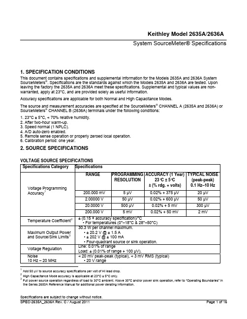
Keithley Model 2635A/2636A System SourceMeter® Specifications1.SPECIFICATION CONDITIONSThis document contains specifications and supplemental information for the Models 2635A and 2636A System SourceMeters ®. Specifications are the standards against which the Models 2635A and 2636A are tested. Upon leaving the factory the 2635A and 2636A meet these specifications. Supplemental and typical values are non-warranted, apply at 23°C, and are provided solely as useful information.Accuracy specifications are applicable for both Normal and High Capacitance Modes.The source and measurement accuracies are specified at the SourceMeters ® CHANNEL A (2635A and 2636A) or SourceMeters ® CHANNEL B (2636A) terminals under the following conditions: 1.23°C ± 5°C, < 70% relative humidity.2.After two-hour warm-up.3.Speed normal (1 NPLC).4.A/D auto-zero enabled.5.Remote sense operation or properly zeroed local operation.6.Calibration period: one year.2.SOURCE SPECIFICATIONSVOLTAGE SOURCE SPECIFICATIONSSpecifications Category SpecificationsRANGE PROGRAMMING RESOLUTION ACCURACY (1 Year) 23°C ± 5°C± (% rdg. + volts) TYPICAL NOISE(peak-peak) 0.1 Hz–10 Hz 200.000 mV 5 µV 0.02% + 375 µV 20 µV 2.00000 V 50 µV 0.02% + 600 µV 50 µV 20.0000 V 500 µV 0.02% + 5 mV 300 µV Voltage Programming Accuracy 1200.000 V5 mV0.02% + 50 mV2 mVTemperature Coefficient 2 ± (0.15 × accuracy specification)/°C•For temperatures (0°–18°C & 28°–50°C)Maximum Output Powerand Source/Sink Limits 3 30.3 W per channel maximum. •± 20.2 V @ ± 1.5 A •± 202 V @ ± 100 mA•Four-quadrant source or sink operation.Voltage Regulation Line: 0.01% of rangeLoad: ± (0.01% of range + 100 µV).Noise10 Hz – 20 MHz< 20 mV peak-peak (typical), < 3 mV RMS (typical) •20 V range1Add 50 µV to source accuracy specifications per volt of HI lead drop.2High Capacitance Mode accuracy is applicable at 23°C ± 5°C only.3Full power source operation regardless of load to 30°C ambient. Above 30°C and/or power sink operation, refer to “Operating Boundaries” in the Series 2600A Reference Manual for additional power derating information.Model 2635A/2636ASystem SourceMeter® SpecificationsSpecifications Category SpecificationsCurrentLimit/Compliance 4 Bipolar current limit (compliance) set with single value. Minimum value is 100 pA. Accuracy is the same as current source. Overshoot< ± (0.1% + 10 mV) (typical )•Step size = 10% to 90% of range, resistive load, maximum current limit/compliance.Guard Offset Voltage< 4 mV•Current < 10 mACURRENT SOURCE SPECIFICATIONSSpecifications Category SpecificationsRANGE PROGRAMMING RESOLUTION ACCURACY (1 Year) 23°C ± 5°C± (% rdg. + amps) TYPICAL NOISE(peak-peak) 0.1 Hz–10 Hz 1.00000 nA 20 fA 0.15% + 2 pA 800 fA 10.0000 nA 200 fA 0.15% + 5 pA 2 pA 100.000 nA 2 pA 0.06% + 50 pA 5 pA 1.00000 µA20 pA 0.03% + 700 pA 25 pA 10.0000 µA 200 pA 0.03% + 5 nA 60 pA 100.000 µA 2 nA 0.03% + 60 nA 3 nA 1.00000 mA 20 nA 0.03% + 300 nA 6 nA 10.0000 mA 200 nA 0.03% + 6 µA 200 nA 100.000 mA 2 µA 0.03% + 30 µA 600 nA 1.00000 A 520 µA 0.05% + 1.8 mA 70 µA 1.50000 A 550 µA0.06% + 4 mA 150 µACurrent ProgrammingAccuracy10.0000 A 5,6 200µA 0.5% + 40 mA (typical)Temperature Coefficient 7± (0.15 × accuracy specification)/°C•For temperatures (0° – 18°C & 28° – 50°C)4For sink mode operation (quadrants II and IV), add 0.06% of limit range to the corresponding current limit accuracy specifications. Specifications apply with sink mode enabled.5Full power source operation regardless of load to 30°C ambient. Above 30°C and/or power sink operation, refer to “Operating Boundaries” in the Series 2600A Reference Manual for additional power derating information.610A range accessible only in pulse mode.7High Capacitance Mode accuracy is applicable at 23°C ± 5°C only.Model 2635A/2636ASystem SourceMeter® SpecificationsSpecifications Category SpecificationsMaximum Output Power and Source/Sink Limits 8 30.3 W per channel maximum. •± 1.515 A @ ± 20 V •± 101 mA @ ± 200 V•Four-quadrant source or sink operation.Current Regulation Line: 0.01% of rangeLoad: ± (0.01% of range + 100pA).VoltageLimit/Compliance 9 Bipolar voltage limit (compliance) set with single value. Minimum value is 20 mV. Accuracy is the same as voltage source. Overshoot< ± 0.1% (typical)•step size = 10% to 90% of range, resistive load•See CURRENT SOURCE OUTPUT SETTLING TIME for additional test conditionsADDITIONAL SOURCE SPECIFICATIONS Specifications Category SpecificationsTransient Response Time< 70 µs for the output to recover to within 0.1% for a 10% to 90% step change in load.Time required to reach within 0.1% of final value after source level command is processed on a fixed range.Range Settling Time 200 mV < 50 µs (typical) 2 V < 50 µs (typical) 20 V < 110 µs (typical) Voltage Source OutputSettling Time200 V < 700 µs (typical)Time required to reach within 0.1% of final value after source level command is processed on a fixed range.•Values below for Iout × Rload = 2 V unless notedCurrent Range Settling Time 1.5 A – 1 A < 120 µs (typical) (Rload > 6 ) 100 mA – 10 mA < 80 µs (typical)1 mA < 100 µs (typical) 100 µA < 150 µs (typical) 10 µA < 500 µs (typical) 1 µA <2 ms (typical) 100 nA < 20 ms (typical) 10 nA < 40 ms (typical) Current Source Output Settling Time1 nA < 150 ms (typical)8Full power source operation regardless of load to 30°C ambient. Above 30°C and/or power sink operation, refer to “Operating Boundaries” in the Series 2600A Reference Manual for additional power derating information.9For sink mode operation (quadrants II and IV), add 10% of compliance range and ±0.02% of limit setting to corresponding voltage source specification. For 200mV range add an additional 120mV of uncertainty.Model 2635A/2636ASystem SourceMeter® SpecificationsSpecifications Category SpecificationsDC Floating Voltage Output can be floated up to ± 250 VDCRemote Sense Operating Range10Maximum voltage between HI and SENSE HI = 3 V Maximum voltage between LO and SENSE LO = 3VVoltage Output Headroom 200 V Range•Maximum output voltage = 202.3 V – total voltage drop across source leads. (maximum 1 Ω per source lead)20 V Range•Maximum output voltage = 23.3 V – total voltage drop across source leads. (maximum 1 Ω per source lead)Over TemperatureProtectionInternally sensed temperature overload puts unit in standby mode.Voltage Source Range Change Overshoot < 300 mV + 0.1% of larger range (typical) •Overshoot into a 200 kΩ load, 20 MHz BWCurrent Source Range Change Overshoot < 5% of larger range + 300 mV/Rload (typical – With source settling set to SETTLE_SMOOTH_100NA)•See CURRENT SOURCE OUTPUT SETTLING TIME for additional test conditions.PULSE SPECIFICATIONSSpecifications Category SpecificationsRegionCircled On Quadrant DiagramMaximumCurrent LimitMaximumPulse Width11MaximumDuty Cycle121 100 mA at 200 V DC, no limit100%1 1.5 A at 20 V DC, no limit 100%2 1 A at 180 V 8.5 ms 1%313 1 A at 200V 2.2 ms 1% Pulse Specifications4 10 A at5 V 1 ms 2.2%10Add 50 µV to source accuracy specifications per volt of HI lead drop.11 Times measured from the start of pulse to the start off-time; see figure below.12Thermally limited in sink mode (quadrants 2 and 4) and ambient temperatures above 30°C. See power equations in the Reference Manual for more information.13Voltage source operation with 1.5 A current limit.Model 2635A/2636ASystem SourceMeter® SpecificationsTypical performance for minimum settled pulse widths: Typical tests were performed using remote opera 14tion, 4W sense, and best fixed measurement range. Fo n on p ripts, e M Source Value Source Sett r more informatio ulse sc see the Series 2600A Referenc anual.Load ling (% of range)Min. Pulse Width5 V 0.5 Ω1%300 µs 20 V 200 Ω0.2%200 µs 180 V 180 Ω0.2% 5 ms 200 V (1.5 A Limit) 200 0.2%Ω 1.5 ms100 mA 200 Ω1%200 µs 1 A 200 Ω1%500 µs 1 A 180 Ω0.2% 5 ms 10 A 0.5 Ω0.5%300 µs 15Times measured from the start of pulse to the start off-time; see figure below.Model 2635A/2636ASystem SourceMeter® Specifications3.METER SPECIFICATIONSVOLTAGE MEASUREMENT SPECIFICATIONS Specifications Category SpecificationsRANGEDISPLAYRESOLUTION18INPUT IMPEDANCE ACCURACY (1 Year)23°C ± 5°C ± (% rdg. + volts) 200.000 mV 1 µV >1014Ω0.015% + 225 µV 2.00000 V 10 µV >1014 Ω0.02% + 350 µV 20.0000 V 100 µV >1014 Ω0.015% + 5 mV Voltage Measurement Accuracy 16,17200.000 V1 mV>1014 Ω0.015% + 50 mVTemperature Coefficient 19± (0.15 × accuracy specification)/°C•For temperatures (0°–18°C & 28°–50°C)16Add 50µV to source accuracy specifications per volt of HI lead drop.17De-rate accuracy specifications for NPLC setting < 1 by increasing error term. Add appropriate % of range term using table below.NPLC Setting 200 mV Range 2 V – 200 V Ranges 100 nA Range 1 µA – 100 mA Ranges 1 A – 1.5 ARanges0.10.01%0.01%0.01%0.01%0.01%0.010.08 %0.07%0.1 %0.05%0.05%0.0010.8 %0.6 %1 % 0.5 % 1.1 % 18Applies when in single channel display mode.19High Capacitance Mode accuracy is applicable at 23°C ± 5°C only.Model 2635A/2636ASystem SourceMeter® SpecificationsCURRENT MEASUREMENT SPECIFICATIONS Specifications Category SpecificationsRANGEDISPLAY RESOLUTION 20VOLTAGEBURDEN 21ACCURACY (1 Year)23°C ± 5°C ± (% rdg. + amps) 100.000 pA 22,23 1 fA < 1 mV 0.15% + 120 fA 1.00000 nA 22,2410 fA < 1 mV 0.15% + 240 fA 10.0000 nA 100 fA < 1 mV 0.15% + 3 pA 100.000 nA1 pA < 1 mV 0.06% + 40 pA 1.00000 µA 10 pA < 1 mV 0.025% + 400 pA 10.0000 µA 100 pA < 1 mV 0.025% +1.5 nA 100.000 µA 1 nA < 1 mV 0.02% + 25 nA 1.00000 mA 10 nA < 1 mV 0.02% +200 nA 10.0000 mA 100 nA < 1 mV 0.02% + 2.5 µA 100.000 mA 1 µA < 1 mV 0.02% +20 µA 1.00000 A 10 µA < 1 mV 0.03% +1.5 mA 1.50000 A 10 µA < 1 mV 0.05% + 3.5 mA Current Measurement Accuracy 1710.000025A100 µA< 1 mV0.4% + 25 mATime required to reach within 0.1% of final value after source level command is processed on a fixed range.•Values below for Vout = 2 V unless notedCurrent Range Settling TimeCurrent Measure 26 Settling Time(Time for measurement to settle after a Vstep) 1 mA < 100 µs (typical)Temperature Coefficient 27± (0.15 × accuracy specification)/°C•For temperatures (0°–18°C & 28°–50°C)20 Applies when in single channel display mode.21Four-wire remote sense only and with current meter mode selected. Voltage measure set to 200 mV or 2 V range only.2210-NPLC, 11-Point Median Filter, < 200V range, measurements made within 1 hour after zeroing. 23°C ± 1°C 23Under default specification conditions: ±(0.15% + 750 fA).24Under default specification conditions: ±(0.15% + 1 pA).2510 A range accessible only in pulse mode.26Delay factor set to 1. Compliance equal to 100 mA.27High Capacitance Mode accuracy is applicable at 23°C ± 5°C only.Model 2635A/2636ASystem SourceMeter® SpecificationsSpecifications Category SpecificationsSpeedMaximum measurement time to memory for 60Hz(50Hz) ACCURACY (1 Year)23°C ± 5°C ± (% rdg. + ohms)Fast 1.1 ms (1.2 ms) 5% + 10 Ω Medium 4.1 ms (5 ms) 5% + 1 Ω Contact Check Specifications 28Slow36 ms (42 ms)5% + 0.3 ΩADDITIONAL METER SPECIFICATIONS Specifications Category SpecificationsMaximum Load ImpedanceNormal Mode 10nF (typical)High Capacitance Mode50uF(typical)Common Mode Voltage 250 VDC Common Mode Isolation >1 G Ω< 4500 pFOverrange101% of source range 102% of measure range Maximum Sense Lead Resistance1 k Ω for rated accuracy Sense High Input Impedance>1014Ω28Includes measurement of SENSE HI to HI and SENSE LO to LO contact resistances.Model 2635A/2636ASystem SourceMeter® SpecificationsHIGH CAPACITANCE MODE 29,30,31Specifications CategorySpecifications Accuracy SpecificationsAccuracy specifications are applicable in both Normal and High Capacitance Modes.Time required to reach within 0.1% of final value after source level command is processed on a fixed range.Current limit = 1AVoltage Source RangeSettling Time withC load = 4.7µF 200 mV600 µs (typical) 2 V600 µs (typical) 20 V1.5 ms (typical) Voltage Source Output Settling Time200 V20 ms (typical) Time required to reach within 0.1% of final value after voltage source is stabilized on a fixed range.•Values below for Vout = 2 V unless notedCurrent Measure RangeSettling Time 1.5 A – 1 A< 120 µs (typical) (Rload > 6 Ω) 100 mA – 10 mA< 100 µs (typical) 1 mA< 3 ms (typical) 100 µA< 3 ms (typical) 10 µA< 230 ms (typical) Current Measure Settling Time1 µA < 230 ms (typical) Capacitor Leakage PerformanceUsing HIGH-C scripts 32200 ms (typical) @ 50 nALoad = 5µF||10M ΩTest: 5V step & measureMode Change Delay100 µA Current Range and above:Delay into High Capacitance Mode: 11 ms Delay out of High Capacitance Mode: 11 ms 1 µA and 10 µA Current Ranges:Delay into High Capacitance Mode: 250 ms Delay out of High Capacitance Mode: 11 ms Voltmeter Input Impedance 30 G Ω in parallel with 3300 pF Noise10 Hz – 20 MHz< 30 mV peak-peak (typical)∙20 V Range29High Capacitance Mode specifications are for DC measurements only. 30100 nA range and below are not available in High Capacitance Mode.31High Capacitance Mode utilizes locked ranges. Auto Range is disabled . 32Part of KI Factory scripts. See the reference manual for details.Model 2635A/2636ASystem SourceMeter® Specifications Specifications Category SpecificationsVoltage Source Range Change Overshoot < 400 mV + 0.1% of larger range (typical) •For 20 V range and below•Overshoot into an 200 k load, 20 MHz BW4.GENERALSpecifications Category SpecificationsIEEE-488 IEEE Std 488.1 compliant. Supports IEEE Std 488.2 common commands and status model topology.RS-232 Baud rates from 300bps to 115200bps.Programmable number of data bits, parity type, and flow control (RTS/CTS hardware or none). When not programmed as the active host interface, the SourceMeter can use the RS-232 interface to control other –instrumentationEthernet RJ-45 connector, LXI Class C, 10/100BT, Auto MDIXLXI Compliance LXI Class C 1.2Total Output Trigger Response Time: 245 µs min., 280 µs typ., (not specified) max.Receive LAN[0-7] Event Delay: UnknownGenerate LAN[0-7] Event Delay: UnknownExpansion Interface The TSP-Link™ expansion interface allows TSP™ enabled instruments to trigger and communicate with each other.Cable Type: Category 5e or higher LAN crossover cable.3 meters maximum between each TSP enabled instrumentUSB USB 2.0 Host ControllerPower Supply 100 V to 250 VAC, 50 Hz – 60 Hz (auto sensing), 250 VA maxModel 2635A/2636ASystem SourceMeter® Specifications Connector: 25-pin female DInput/Output Pins: 14 open drain I/O bitsModel 2635A/2636ASystem SourceMeter® Specifications Specifications Category SpecificationsCooling Forced air. Side intake and rear exhaust. One side must be unobstructed when rack mountedWarranty1yearEMC Conforms to European Union Directive 2004/108/EEC, EN 61326-1Safety Conforms to European Union Directive 73/23/EEC, EN 61010-1, and UL 61010-1Dimensions 89 mm high × 213 mm wide × 460 mm deep (31⁄2 in × 83⁄8 in × 171⁄2 in). Bench Configuration (with handle & feet): 104 mm high × 238 mm wide × 460 mm deep (41⁄8 in × 93⁄8 in × 171⁄2 in)Weight 2635A: 4.75 kg (10.4 lbs). 2636A: 5.50 kg (12.0 lbs).Environment For indoor use only.Altitude: Maximum 2000 meters above sea levelOperating: 0°– 50°C, 70% R.H. up to 35°C. Derate 3% R.H./°C, 35°– 50°C Storage: – 25°C to 65°CModel 2635A/2636ASystem SourceMeter® Specifications 5.MEASUREMENT SPEED SPECIFICATIONS33,34,35Maximum Sweep Operation Rates (operations per second) for 60Hz (50Hz):A/D converterspeed TriggeroriginMeasure tomemoryusinguser scriptsMeasure toGPIBusinguser scriptsSourcemeasure tomemoryusinguser scriptsSourcemeasure toGPIBusinguser scriptsSourcemeasure tomemoryusingsweep APISourcemeasure toGPIBusingsweep API0.001 NPLC Internal 20000 (20000) 9800 (9800) 7000 (7000) 6200 (6200)12000(12000)5900 (5900)0.001 NPLC Digital I/O 8100 (8100) 7100 (7100) 5500 (5500) 5100 (5100)11200(11200)5700 (5700)0.01 NPLC Internal 4900 (4000) 3900 (3400) 3400 (3000) 3200 (2900) 4200 (3700) 4000 (3500)0.01 NPLC Digital I/O 3500 (3100) 3400 (3000) 3000 (2700) 2900 (2600) 4150 (3650) 3800 (3400)0.1 NPLC Internal 580 (480) 560 (470) 550 (465) 550 (460) 560 (470) 545 (460)0.1 NPLC Digital I/O 550 (460) 550 (460) 540 (450) 540 (450) 560 (470) 545 (460)1.0 NPLC Internal 59 (49) 59 (49) 59 (49) 59 (49) 59 (49) 59 (49)1.0 NPLC Digital I/O 58 (48) 58 (49) 59 (49) 59 (49) 59 (49) 59 (49) Maximum Single Measurement Rates (operations per second) for 60Hz (50Hz):A/D converterspeed TriggeroriginMeasure to GPIBSource measureto GPIBSource measure pass/fail to GPIB0.001 NPLC Internal 1900 (1800) 1400 (1400) 1400 (1400)0.01 NPLC Internal 1450 (1400) 1200 (1100) 1100 (1100)0.1 NPLC Internal 450 (390) 425 (370) 425 (375)1.0 NPLC Internal 58 (48) 57 (48) 57 (48)Maximum measurement range change rate: >7000/second for >10 µA typical. When changing to or from a range ≥1A, maximum rate is >2200/second typical.Maximum source range change rate: >400/second >10 µA typical. When changing to or from a range ≥1A, maximum rate is >190/second typical.Maximum source function change rate: >1000/second, typical.Command processing time: Maximum time required for the output to begin to change following the receipt of the smux.source.levelv or smux.source.leveli command. <1ms typical.33 Tests performed with a 2636A on Channel A using the following equipment: Computer hardware (Intel® Pentium® 4 2.4 GHz,2 GB RAM, National Instruments™ PCI-GPIB). Driver (NI-488.2 Version 2.2 PCI-GPIB). Software (Microsoft® Windows® XP,Microsoft® Visual Studio® 2010, VISA™ version 4.1).34 Exclude current measurement ranges less than 1mA.35 2635A/2636A with default measurement delays and filters disabled.Model 2635A/2636ASystem SourceMeter® Specifications6.TRIGGERING AND SYNCHRONIZATION SPECIFICATIONSTriggering:Trigger in to trigger out: 0.5μs, typical.Trigger in to source change:3610 μs, typical.Trigger Timer accuracy: ±2μs, typical.change36 after LXI Trigger: 280μs, typical.SourceSynchronization:Single-node synchronized source change:36<0.5μs, typical.Multi-node synchronized source change:36<0.5μs, typical.7.SUPPLEMENTAL INFORMATIONFront Panel Interface:Two-line vacuum fluorescent display (VFD) with keypad and rotary knob.Display:∙Show error messages and user-defined messages∙Display source and limit settings∙Show current and voltage measurements∙View measurements stored in dedicated reading buffersKeypad operations:∙Change host interface settings∙Save and restore instrument setups∙Load and run factory and user-defined test scripts (i.e., sequences) that prompt for input and send results to the display∙Store measurements into dedicated reading buffersProgramming:Embedded Test Script Processor (TSP): Accessible from any host interface.∙Responds to individual instrument control commands.∙Responds to high-speed test scripts comprised of instrument control commands and Test Script Language (TSL) statements (for example branching, looping, and math).∙Able to execute high-speed test scripts stored in memory without host intervention.Minimum user memory available: 16MB (approximately 250,000 lines of TSL code).Test Script Builder: Integrated development environment for building, running, and managing TSP scripts. Includes an instrument console for communicating with any TSP-enabled instrument in an interactive manner. Requires:∙VISA (NI-VISA included on CD)∙Microsoft .NET Framework (included on CD)∙Keithley I/O Layer (included on CD)36Fixed source range, with no polarity change.Model 2635A/2636ASystem SourceMeter® Specifications TSP™ Express (embedded):Tool that allows users to quickly and easily perform common I-V tests withoutprogramming or installing software. To run TSP Express, you need:∙Java™ Platform, Standard Edition 6∙Microsoft® Internet Explorer®, Mozilla® Firefox®, or another Java-compatible web browserSoftware Interface: TSP Express (embedded), direct GPIB/VISA, read/write with Microsoft® Visual Basic®, Visual C/C++®, Visual C#®, LabVIEW™, CEC TestPoint™ Data Acquisition Software Package, NI LabWindows™/CVI, and so on.Reading Buffers:Non-Volatile memory utilizes dedicated storage area(s) reserved for measurement data. Reading buffers are arrays of measurement elements. Each element can hold the following items:∙Measurement∙Source setting (at the time the measurement was taken)∙Measurement status∙Range information∙TimestampTwo reading buffers are reserved for each SourceMeter channel. Reading buffers can be filled using the front panel STORE key, and retrieved using the RECALL key or host interface.Buffer Size, with timestamp and source setting: > 60,000 samples.Buffer Size, without timestamp and source setting: > 140,000 samples.System Expansion:The TSP-Link expansion interface allows TSP-enabled instruments to trigger and communicate with each other. See figure below:Model 2635A/2636ASystem SourceMeter® SpecificationsEach SourceMeter has two TSP-Link connectors to make it easier to connect instruments together in sequence.∙Once SourceMeter instruments are interconnected via TSP-Link, a computer can access all of the resources of each SourceMeter via the host interface of any SourceMeter.∙ A maximum of 32 TSP-Link nodes can be interconnected. Each SourceMeter consumes one TSP-Link node.TIMER:Free-running 47-bit counter with 1MHz clock input. Reset each time instrument powers up. Rolls over every 4 years.Timestamp: TIMER value automatically saved when each measurement is triggered.Resolution: 1μs.Timestamp Accuracy: ±100ppm.。
MCR-WPT发射接收线圈性能仿真建模分析
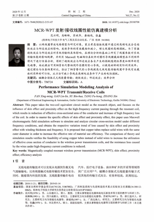
2020年12月第27卷第12期控制工程Control Engineering of ChinaD ec.2020Vol.27,N o.12文章编号:1671-7848(2020)12-2151-07 DOI: 10.14107/ki.kzgc.20180708M CR-W P T发射/接收线圈性能仿真建模分析范兴明,高琳琳,苏斌华,唐福鸿,张鑫(桂林电子科技大学电气工程及其自动化系,广西桂林541004)摘要:以两线圏等效电路模型为研究对象,重点考虑谐振线圈中通过的高频电流会受趋肤效应与邻近效应的影响,致使导体的有效截面积减小,增大线圈的高频损耗。
为了掌握 K:趋肤效应与邻近效应对系统传输的具体影响,在理论分析的基础上研究了线圏参数对系统 ^ 传输性能的影响规律,并利用M a x w e丨丨电磁场仿真软件对圆形导线横截面模型在不同频率情况下进行仿真分析,得到了趋肤效应与邻近效应各自产生的损耗随绕组厚度和频率的变丨化趋势,由此提出可用铜管来代替相同外径圆形实心导线,以提高材料的实际利用效率。
通过理论与仿真结果对比,验证了铜管替代实心导线提高无线电能传输线圈中导线有效截面利用率的可行性,此方法可减小导线在高频电流条件下产生的电阻损耗。
关键词:磁耦合谐振式无线能量传输:趋肤效应;邻近效应;效率分析中图分类号:TM724 文献标识码:APerformance Simulation Modeling Analysis ofMCR-WPT Transmit/Receive CoilsF A N X in g-m ing,G AO Lin-lin,S U B in-hua,TANG F u-hong,ZH A N G X in(Department of Electrical Engineering&Automation,Guilin University of Electronic Technology,Guilin541004, China) Abstract: This paper takes the two-coil equivalent circuit model as the research object, and focuses on the influence of skin effect and proximity effect on the high-frequency current passing through the resonant coil, which resu lt s in reduction of effective cross-sectional area of the conductor and increase of high frequency loss of the coil. In order to master the specific effects of skin effect and proximity effect, t h is paper uses Maxwell electromagnetic f ield simulation software to simulate and analyze circular cross-section model under different frequency conditions, and obtains the respective variation trend of loss caused by skin effect and proximity effect with winding thickness and frequency.I t i s proposed that copper tubes replace solid wires with the same outer diameter i n order to increase the effective rate of material use efficiency. The comparison of theory and simulation results verifies the f e as ib il it y of using copper tubes instead of solid wires to increase the utilizati on of effective cross section of conductor i n the wireless power transmission coils, and the resistance loss caused by the wires under high-frequency current conditions i s reduced.Key words: Magnetically coupled resonant wireless power transmission (M C R-W P T); skin effect; proximity effect;efficiency analysisi引言无线电能传输技术可以实现从电源到负载无电汽车、医疗电子设备、油田和矿井的开采等领域得 气接触输电,比传统接触式电能传输技术更加安全。
海沃德游泳池清洁器说明书

2Limited WarrantyMakoShark 2KingSharkKingShark 2KingShark 2 w/RemoteTigerShark 2Tiger Shark 2 PlusYour Hayward Pool Cleaner has been manufactured, tested and inspected in accordance with carefully specified engineering requirements. It is warranted to be free from defects in materials and workmanship for a period of one year. Coverage is provided to the original owner only and is not transferrable. This limited warranty includes both parts and labor for the cleaners listed above. This warranty gives you specific legal rights. You may also have other rights, which vary from state to stateEXCEPTIONS AND EXCLUSIONS FROM WARRANTYDamage, malfunctions orrising from improper electrical supply levels are excludedfrom this warranty. Malfunctions, failure or damage of the cleaner caused by improper, unreasonable, or negligent use or abuse by the consumer, are excluded from this warranty.Any repair that is made on your cleaner during the warranty period by anyone other than an Authorized Hayward Warranty Service Center (designated to perform such work) will void this warranty and other warranty rights you may have. Filter cartridges and debris bags are not covered by this warrantyINSTRUCTIONS TO OBTAIN WARRANTY REPAIRTo obtain repair of your Hayward cleaner under this warranty, the following procedure must be followed:• Locate and deliver the cleaner to the nearest Hayward Factory Authorized Warranty Service Center. Your Authorized Hayward Warranty Service Center can be located by visiting . You may also call 908-355-7955 to locate you nearest authorized service center. Cost of transportation, if required, is at the sole expense of the owner. Proof of purchase is required.TERMSIf a warranty claim is made and the product delivered to an Authorized Hayward Warranty Service Center within the warranty period, your Hayward cleaner will be repaired at no charge (parts & labor) to you. Listed warranty exclusions apply.No dealer, distributor, or other similar person has any authority to make any warranties or representations concerning Hayward Pool Cleaner products or to extend this warranty beyond the express items contained herein. Accordingly, Hayward Pool Products assumes no responsibility for any such warranties or representations beyond the express items contained in this limited warranty.WARRANTY REGISTRATION CARDYou can register your unit on-line by visiting or by filling out the registrationcard and returning it to:Hayward IndustriesAttn Warranty Department620 Division StreetElizabeth, NJ 07207CONTENTSSafety Precautions (2)General Information (3)Motor Information (4)Trouble Shooting (5)Specifications (7)Machine Assembly/Parts (8)Filter Assembly/Parts (10)Accessories (11)Preventive Maintenance (13)Parts Ordering Instructions (14)SAFETY PRECAUTIONSThe KingShark2 automatic swimming pool vacuum cleaner has been manufactured with the highest degree of care and concernfor safety. We suggest the following safety precautions become part of your pool safety regulations:1. ALWAYS PUT THE MACHINE INTO THE WATER BEFORE CON-NECTING IT TO THE ELECTRICAL OUTLET.2. IT IS IMPORTANT FOR SWIMMERS’ SAFETY TO REMOVETHE UNIT IMMEDIATELY FOLLOWING USE. THIS WILL ALSOIMPROVE THE OPERATING LIFE OF YOUR KING SHARK2.3. BE CERTAIN THE MACHINE IS ONLY PLUGGED INTO AGROUNDED ELECTRICAL OUTLET EQUIPPED WITH AGROUND FAULT CIRCUIT INTERRUPTER.4. DO NOT HANDLE MACHINE WHILE IT IS PLUGGED INTO THEELECTRICAL OUTLET.5. DO NOT USE AN EXTENSION CORD. THIS COULD CREATE ASAFETY HAZARD AND/OR DAMAGE YOUR UNIT.6. ALWAYS STAY OUT OF THE POOL WHILE CLEANER IS INOPERATION.7. NEVER ALLOW PLUG TO ENTER THE POOL.8. DO NOT OPERATE THE MACHINE OUT OF WATER. THIS WILLDAMAGE THE MOTOR SEAL AND VOID THE WARRANTY.9. DO NOT DRAG THE MACHINE OUT OF THE POOL AGAINSTTHE SIDE WALL. THIS COULD DAMAGE UNIT AND/OR YOURPOOL WALL.10. SOME POOLS HAVE A CORNER OR A CORNER STEP CON-FIGURATION THAT MAY CAUSE THE UNIT TO “HANG-UP;”THEREFORE, DO NOT LEAVE THE UNIT COMPLETELYUNATTENDED FOR MORE THAN 1/2 HOUR. OCCASIONALOBSERVATION AND ATTENDANCE CAN ALSO REDUCE ANYTENDENCY FOR THE CORD TO TWIST.While the KingShark2 has been made to operate as safely as possible, we suggest you exercise reasonable care in the handling of the vacuum and inspect the electrical cord frequently for damage or wear, as with any other electrical appliance. After use, remove the unit and rinse with fresh water and remove any twists that may be present in the cord.GENERAL INFORMATIONYou have purchased the finest piece of equipment in the pool cleaner industry. If you treat it as such, your KingShark2 automatic swimming pool vacuum cleaner will give you years of satisfactory service. As a suggestion, the unit should be stored in the original shipping container for safekeeping during the off season.ADJUSTMENTTHERE IS ONE ADJUSTMENT THAT MAY BE NECESSARY FOR USE IN YOURPOOL. PLEASE TAKE THE FEW MINUTES NECESSARY TO UNDERSTAND THIS SIMPLE PROCEDURE:1.2.3.4.1.2.3. The height of the sensor bar #3210 (Page 9, Key 2) is pre-set at the factory for average pools. It may be necessary to readjust the height of the sensor bar for the machine to operate satisfactorily in your pool.In “Free Form” or “Bowl Shaped” pools, the sensor bar may have to be raised to a higher setting to allow the machine to climb out of the deep end and clean up the radius or slope as far as possible without the machine turning over.Adjustment of the sensor bar #3210 (Page 9, Key 2) is made by loosening adjust- ing arm bolts #2121 B (Page 9, Key D) located just ahead of the intake. With the machine sitting on a level surface, loosen both adjusting arm bolts, and move sensor bar to desired position. Make certain the sensor bar is parallel to the level surface and retighten the adjusting arm.It may be necessary to reset the sensor bar several times to find the best position for operation in your pool. Sensor bar should glide freely. This can be checked by pushing back on the sensor bar which will activate the reversing arms.OPERATING INSTRUCTIONSSelect nearest grounded outlet supply of 110/115/220/240 voltage.CAUTION: avoid overloaded circuits as low or high voltage can damage your mo- tor. A connected ground is most important. Plug into outlet. Observe machine as it travels over bottom of pool.Allow machine to travel around the pool until it is clean. Average 75' x 150' pool will required approximately 4 hours. If the pool has a heavy accumulation of debris, it may be necessary to clean the filter several times during the vacuuming period. Upon completion of vacuuming the pool, allow the unit to travel to the shallow endof the pool. Before it reaches the pool wall, turn power off, raise the unit by the white nylon rope #1312, then remove the unit from the water by use of the handle. Allow excess water from the filter to drain into the pool with the KingShark2 resting on the edge or coping. Do not leave machine in water after disconnecting.4.5.6.7.8.KingShark2REMOVE THE UNIT IMMEDIATELY AFTER USE.ALLOWING UNIT TO COOL IN WATER AFTERRUNNING CAN CAUSE MOTOR SEAL DAMAGE.To clean the cartridge filters #7807 (Page 10, Key 7) remove the filter housing assembly #3400 (Page 10, Key 13) by removing the filter knob and releasing the filter box.Cleaning the filters after each use is an important part of maintaining your King- Shark2. Clean filters will allow the machine to function most efficiently.Disassemble the filter housing assembly #3400 (Page 10, Key l3) by removing the four (4) filter knobs #3405 (Page 10, Key 3) The filter backplate #3416 (Page 10, Key 10) and filter cartridges #7807 can then be removed.Clean cartridges with a water hose using a pressure nozzle.Use the KingShark2 on a regular basis to keep your pool clean.MOTOR INFORMATIONThe Motor in your KingShark2 has automatic overload protection. The overload switch will protect the motor against burning out when an obstruction stops the machine. When an obstruction stops the machine, UNPLUG THE CORD FROM THE OUTLET and remove the unit from the pool. Turn the machine over and with the aid of a long screw driver or needle-nose pliers, rotate the impeller and dislodge any foreign object. All large objects should be removed from the pool before the KingShark2 is put into operation.KingShark2TROUBLE SHOOTINGWhere to set Sensor Bar(Make adjustments in 1/4" Increments)Machine fails to come out of deep end:Raise sensor bar to allow the machine to climb the incline to shallow end. Machine turns in circles and twists cord:1.2.3.4.5. Sensor bar too high, hitting hood, or is not level.Thread on reversing arm #2203 (Page 9, Key 16) is worn or stripped, not allowing reversing mechanism to disengage.Drive wheel broken.Drive belt broken.Is the unit being run in the pool for too great a length of time? Four hours in operation in the larger pools should be sufficient with not more than a few twists in the cord, which should be straightened out after each vacuuming.Machine does not pick up:1.2. Filter may be clogged and not permitting the flow of water through the filter cartridges, (clean filter cartridges).Large object lodged in the intake or in the impeller housing (remove object).Machine does not move:1.2.3.Not connected to live outlet, (check electrical source).Object lodged in impeller, (remove object).A short in the motor, (check the ground fault interrupter for tripping).4.5.TROUBLE SHOOTINGUnit runs for short distance but stops. Check for overloaded circuit or possible faulty motor. *Contact service center*(DO NOT USE EXTENSION CORDS.)Motor runs but unit becomes motionless (gear box worm is worn or the drive pin is sheared).Machine tips over backwards before sensing wall:1.2.3. Improper sensor bar adjustment, (too high).Cord too short for pool length. *Contact service center.*You may need optional float Part No. 7 (Page 13 ) call factory or local dealer/service center.Machine tips over before tripping or sensing wall:1. Lower sensor bar to ensure it will engage and reverse unit.KEEP SENSOR BAR LEVEL AT ALL TIMES!MOTOR:SPECIFICATIONSType ...................................................................... Submersible EXPORT ONLY Voltage .................................................................. 110/115 Volts ................................ 230/240 VoltsFrequency ............................................................. 60 Cycle ...........................................60/50 CycleSpeed .................................................................... 1725 RPM ..........................................1425 RPMBearing .................................................................. Ball BearingsHousing ................................................................. Aluminum AnodizedMotor Seals ........................................................... Double Lip WaveOverload Protection .............................................. Thermal OverloadElectrical Cord ....................................................... #16 Wire Encased in Flotation Jacket; 150' in lengthDRIVE:Rear Wheel Drive ................................................. Planetary Gear SystemFront Wheel Driven by .......................................... Continuous BeltFILTER:Type ...................................................................... Self ContainedFilter Media ........................................................... Corrugated Resin Impregnated ElementPorosity ................................................................. 50 MicronsFilter Area .............................................................. 40 Square FeetHousing ................................................................. Molded PlasticGallons Circulated ................................................. 70-75 Per Minute/4200-4500 Per HourSHAFT and AXLE:All parts such as axle, shafts, pins, fasteners, rods, etc., are corrosion resistant.(KingShark2) SPECIFICATIONS WITHOUT SWIVELUNIT DIMENSIONS Height 15 in. (38.1 cm) Width 24 in. (60.0 cm) Length 29 in. (73.6 cm)UNIT WEIGHT86.5 lbs. (39.2 Kg)UNIT CORD LENGTH150 ft. (45.7m)UNIT DIMENSIONS (KingShark2) SPECIFICATIONS WITH SWIVELUNIT WEIGHT UNIT CORD LENGTHHeight 19.5 in. (49.5cm)Width 24 in. (60.0 cm)Length 29 in. (73.6 cm)89.0 (40.5 Kg) 150 ft. (45.7m)UNIT BOX DIMENSIONS (KingShark2) W/BOX SPECIFICATIONSUNIT BOX WEIGHT UNIT BOX VOLUMEHeight 19.5 in. (49.5 cm) W/Swivel 23.5 in. (59.7 cm) Width 26.0 in. (66.0 cm) Length 32.0 in. (81.3 cm) 105 lbs. (47.6 Kg)109 lbs. (49.4 Kg)w/optional Swivel9.38 ft3 (.3m3)11.31 ft3 (.36m3)w/optional SwivelCART BOX DIMENSIONS CADDY CART W/BOX SPECIFICATIONSCADDY CART WEIGHT CART BOX VOLUMEHeight 12.5 in. (31.8 cm) Width 22.5 in. (57.2 cm) Length 42.5 in. (107.0 cm) 16.5 lbs. (7.5 Kg)WITH BOX29.0 lbs. (13.2 kg)6.92 ft3 (0.2m3)KingShark2WITH SWIVEL89I T H S W I V E LKingShark2 HOOD & FILTER ASSEMBLYKEY PART NO. 1-A 3310GPART DESCRIPTIONHOOD - GREY PLASTICREQ L/H R/H11 3310GS SWIVEL HOOD - GREY PLASTIC 12 3309A 212B3 34054 34095 3401C 34026 3403D 34027 78078 7813 SPACER - HOOD MOUNTINGBOLT HEX HD 1/4-20X3/4" SSKNOB - FILTERKNOB - FILTER ASSEMBLYINTAKE - FILTER HOUSINGSCREW PHIL HD #4X3/8" SSBAFFLE - FILTER HOUSINGSCREW PHIL HD #4X3/8" SSFILTER - CARTRIDGEGASKET FOAM 1/4" OVAL4 2 22 1 14 2 2114 2 212 1 14 2 28 4 49 7808PC TIE ROD - FILTER 4 2 210 341611 341112 3410E 3402 PLATE - BACK ASSEMBLYPLATE - REINFORCING BACK(REFERENCE ONLY)PLATE - BACK (REF. ONLY)SCREW PHIL HD #4X3/8" SS1114 2 213 3400 FILTER ASSEMBLY - COMPLETE 110KingShark2ACCESSORIES11KingShark2ACCESSORIESCADDY CART12KingShark2KingShark2PREVENTATIVE MAINTENANCECongratulations on the purchase of the KingShark2. The KingShark2 is built and designed to give you years of service.In order to maximize efficiency and receive long term service, we suggestthe following:2.3.4.5.6. Thoroughly rinse entire unit after use.Clean filters thoroughly after each use - a clogged filter will decreaseefficiency dramatically.Remove any twists in the cord after each use. Twisting should be minimalif the unit is functioning properly.Avoid allowing the unit to “cool down” in the water. For example, if used on a timer, it is better to set for 3:00 a.m. to 8:00 a.m. (then remove) thanit is to set for 12:00 a.m. to 5:00 a.m. (and remove it at 8:00 a.m.). Inspect belts and filter frequently. Replace when necessary.Always keep your Sensor Bar level; (a non-level Sensor Bar can cause the cord to twist).Protect Your Investment!Following these quick and easy steps will extend the life and efficiency of your KingShark2.13KingShark2PARTS ORDERING INSTRUCTIONSShould you desire to order repair parts, follow this simple procedure:1.2.3.4.5. Ascertain each of the parts you will need and identify them by part number. Use this book as a guide; be sure to note that in some cases, due to continual product improvement, parts may vary depending on the time of manufacture.Contact your local Factory Authorized Service Center with the listof parts you will need. Be sure to advise the Service Center of the KingShark2 serial number and the date of purchase. If you need the location of your nearest Service Center, go to the or call Hayward, 908-351-5400All parts will be shipped immediately via best way on a collect freight basis, from the Service Center.All shipments will be C.O.D. unless prior arrangements have been made with the service centerAll parts under limited warranty are confined to the specific limitations as stated.14MakoShark 2TigerSharkFOR RESIDENTIAL POOLSThe MakoShark 2 and TigerShark are portable automatic vacuum cleaners. THERE IS NO INSTALLATION! Several hours eachweek will enable the M a koShark 2 and TigerShark to keep your pool spotless. NO WHIPS, NO PIPES OR EXTRA PLUMBING. Remember, when you really clean your home, you don't just sweep or dust, you vacuum. There is no better way to cleanyour home pool than with… the MakoShark 2 or TigerShark.。
- 1、下载文档前请自行甄别文档内容的完整性,平台不提供额外的编辑、内容补充、找答案等附加服务。
- 2、"仅部分预览"的文档,不可在线预览部分如存在完整性等问题,可反馈申请退款(可完整预览的文档不适用该条件!)。
- 3、如文档侵犯您的权益,请联系客服反馈,我们会尽快为您处理(人工客服工作时间:9:00-18:30)。
a r X i v :c o n d -m a t /0207654v 1 [c o n d -m a t .s o f t ] 26 J u l 2002Two-level system with a thermally fluctuating transfer matrix element:Application tothe problem of DNA charge transferMaria R.D’Orsogna and Joseph RudnickPhysics Department,University of California,Los Angeles,CA 90095-1547(Dated:February 1,2008)Charge transfer along the base-pair stack in DNA is modeled in terms of thermally-assisted tunneling between adjacent base pairs.Central to our approach is the notion that tunneling between fluctuating pairs is rate limited by the requirement of their optimal alignment.We focus on this aspect of the process by modeling two adjacent base pairs in terms of a classical damped oscillator subject to thermal fluctuations as described by a Fokker-Planck equation.We find that the process is characterized by two time scales,a result that is in accord with experimental findings.PACS numbers:87.15.-v,73.50.-h,82.30.FiI.INTRODUCTIONIn spite of the fact that a decade has passed since the first definitive observation of charge transfer along the DNA base-pair stack [1],the detailed properties of this process have not been definitively elucidated.This is partly due to the inherent complexity of the molecular structure of DNA,and to the large number of exter-nal and intrinsic factors that exert an influence on DNA structure and behavior.The current unsettled situation also reflects the absence of an overall agreement on the precise mechanism by which this charge transport takes place.One of the key issues that awaits full illumina-tion is the role of disorder—both static and dynamic—on the propagation of charge along the base-pair stack.A related,and quite fundamental,question is whether charge transport is a coherent quantum mechanical pro-cess,like conduction of electronic charge against a static,or deformable,background,or whether it it takes place as fundamentally incoherent transport,as a variation of the random walk.The answers to these and other questions will have a significant impact on both our understand-ing of the biological impact of charge transport in DNA and the development of applications based on this phe-nomenon.Despite the often contradictory results of experimen-tal investigations [2,3,4,5,6],a few conclusions seem inescapable.The first is that long-range charge trans-port along the base-pair stack depends quite strongly on the sequence of the base pairs [7].In addition,base-pair mismatches can have a significant deleterious effect on charge transport [8,9](see,however [10]).Furthermore,strands of DNA display considerable disorder,both static [11]and dynamic [12,13,14,15].Finally,several sets of experiments on ensembles of short DNA strands have uncovered an unusual two-step charge transfer process [16,17].These studies focus on fluorescent charge donors intercalated in DNA oligostrands.As the charge migrates towards the acceptor,the fluorescence is quenched and the rate of migration is determined by the decaying flu-orescence profile.The data reveals that this decay pro-cess occurs according to two characteristic time-scaleswhich are separated by more than an order of magni-tude [16,17].Any model that purports to explain charge transport must take all this into account.In this paper,we discuss a model for short range charge transport along a base pair stack that undergoes substantial structural fluctuations.The process occurs via thermally-assisted quantum mechanical tunneling of charge carriers from one base pair to the next,under the assumption that this tunneling is properly character-ized as occurring in the presence of a dissipative environ-ment.A key conjecture is that charge transfer takes place only when the neighboring pairs are in a state of optimal “alignment”,and that this alignment is statistically un-likely in thermodynamic equilibrium.As we will see,this conjecture leads in a natural way to a model exhibiting the dual-time-scale feature described above.Addition-ally,the model generates predictions that can be readily tested.We shall relate the problem at hand to the dy-namics of a simple two level system (TLS),realized by a donor and an acceptor state.In Section II,we briefly recapitulate what is known about the tunneling process in the presence of friction for a TLS system.We also quantify our notion of a coordi-nate θassociated with the “alignment”of adjacent base pairs and of the influence of the dynamics of this new coordinate on charge transfer.Section III specifies the model for describing a generic collection of two-level sys-tems (TLS),initially in the donor state and characterized by a fluctuating alignment variable θ.The probabilitydistribution of donor states,W (θ,˙θ,t )obeys a Kramers equation with a sink term due to charge transfer to the acceptor.The rate of charge transfer will be expressed by the fluctuating rate Γ(θ).This Kramers expression is recast into the form of a Volterra equation with the use of a Lie-Algebra approach defined on the Hilbert space of the eigenstates of the Kramers equation for Γ(θ)=0.We will discuss limiting cases of the solution to obtain physical insight and to reveal the two-time-scale decay of the probability distribution due to the sink term.We conclude in Section IV with a discussion of the possible application of our results to charge transfer in strands of DNA consisting of several base pairs.The key result of our calculations lies in the determi-2nation of P(θ∗,t),the probability distribution of donor states evaluated at the optimal configurationθ∗and with the˙θvariable integrated out.Indeed,under the assump-tion that the tunneling process is most effective atθ∼θ∗, this quantity is directly related to thefluorescence in-tensity I(t)of the base pair complexes,as probed by J. Barton and A.Zewail[16,17],through the following:I(t)=I0 1−Γ t0P(θ∗,t′)dt′ .(1)The quantity I0of the above relationship is a propor-tionality constant andΓis the integrated rate of transfer to the acceptor.We shall determine the double expo-nential character of P(θ∗,t),and hence of I(t),in qual-itative agreement with the experimentalfindings.The conjectures made on the existence of an optimal and un-likely configurationθ∗will be crucial in obtaining the two stage decay process,a result that justifies the as-sumptions made.The model we shall construct is obviously not re-stricted in application to DNA ing our results,we may conclude that in an ensemble of generic systems the migration of a particle from donor to ac-ceptor proceeds statistically as a two-time scale process, provided the transfering process is of rare occurrence.II.THE TUNNELING PROCESSThe process of charge transfer from a donor site to an acceptor site—a two-level system—is ubiquitous in bio-chemical and physical phenomena[18].It occurs under a broad variety of spatio-temporal conditions.Chemical bond formation or destruction,ATP production in pho-tosynthetic reactions,or the operation of semiconduct-ing devices,all involve the transfering of charges to and from specific sites,via thermal activation or quantum-mechanical tunneling through an energy barrier.Be-cause of its intrinsic nature,charge transfer via quantum-mechanical tunneling takes place on a length scale of up to tens of angstroms[19];larger distances are possible if other transport mechanisms are involved.These in-clude thermal hopping among sites,which are typical in disordered systems,the creation of conduction bands in metals,or of lattice distortions of polaronic type in spe-cific systems.Quantum-mechanical tunneling from a donor site to an acceptor site is quite simply represented by a two-level system(TLS)[20].In this description,the tunneling particle is limited to being in the donor or in the acceptor state,while the other degrees of freedom of the system, nuclear for instance,describe the charge potential energy. The energetic profile of the system is thus characterized by a multidimensional surface of which the acceptor and the donor states constitute relative minima,separated by a barrier.Of the many existing degrees of freedom,it is often possible to identify a“reaction coordinate”ysuchyFIG.1:Thisfigure illustrates the nature of the tunneling transition.The two parabolic curves shown correspond to the two versions of the potential V(y,σz)in Eq.(2),one corresponding to the“donor”state in which the tunneling particle is on one site and the other to the“acceptor”state, in which the particle is on the other one.The two energies E f and E b=E f−ǫreferred to in the text are the forward and backwards barrier energies respectively.The horizontal axis corresponds to the reaction coordinate,y.that the energy barrier between donor and acceptor is minimized along this specific direction.The progress of the reaction is then dominated by the evolution along this coordinate and the potential energy surface can be reduced to an effective one-dimensional curve.In certain systems the physical interpretation of the reaction coordinate is immediate:it may be the relative bond length in two diatomic molecules,or solvent polar-ization around the donors and acceptors[21].It is not an easy task to give a physical interpretation of the re-action coordinate in the case of DNA base pairs because of the many possibilities involved-intra-base distance, mobile counter-ion concentration,solvent concentration, or a combination of all the above.A possibility is offered by Ref.[22]where it is suggested that the most relevant quantity is the interaction of the charge with the polar water molecules of the solvent.In this paper we shall refer to the reaction coordinate y in most general terms.A common representation of tunneling with dissipation is through the spin-boson formalism[20].The donor and acceptor states are represented by means of a pseudo spin,which points up when the charge is in the donor state and down otherwise.The Hamiltonian of the sys-tem is given by:H ET=τσx+P2y2Mω2(y+y0σz)2+13 andσx,z are the Pauli matrices.The charge in the donor(up)state corresponds to the potential V(y,+)whoseequilibrium reaction coordinate is−y0,and the conversestate corresponds to V(y,−),whose stable minimum isat y0.The H bath term represents contributions to theHamiltonian of a dissipative environment coupled to thereaction coordinate.Figure1illustrates the meaningof the potential V(y,σz)in the effective Hamiltonian ofEq.(2).The curve marked A corresponds to the poten-tial term in the donor state,while the curve marked Brepresents the potential function in the acceptor state.This model has been thoroughly analyzed in the workby Garg e t al.[23]based on earlier work by Leggett[24].A similar analysis,but within a more chemical frame-work,is presented by Marcus e t al.[25].Energy con-servation requires that charge transfer takes place onlywhen the reaction coordinate is close to the degeneracypoint y=y∗for which V(y∗,+)=V(y∗,−);once thedegeneracy point is reached,charge transfer is possibleonly because of the non zero off-diagonal tunneling ma-trix elementsτ.The tunneling rateΓfrom donor to acceptor,is calcu-lated in the above references.For moderate dissipationof the reaction coordinate,it is given by:Γ=τ2E r k B T eff 14 III.THE TLS ANDθFLUCTUATIONSA.The modelConsider a collection of TLS which at the initial time t=0are all in the up-donor configuration,and charac-terized by the angular parameterθ.Let us denote by W(θ,˙θ,t)the TLS population remaining in the up-donor state at time t and for which the collective angular vari-able and its velocity are specified.The physical requirement thatθbe randomly,classi-cally,fluctuating in time,translates into the fact that W(θ,˙θ,t)must evolve according to a Fokker-Planck type equation as dictated by standard Langevin theory.To this probability evolution equation we must add an addi-tional depleting term,that which represents tunneling to the donor site as given by theΓ(θ)term discussed above. Different scenarios are possible for theθdependence of τand hence ofΓ.As discussed in the above section we shall focus on the particular situation in which tunneling is possible only for a very specific subset of energetically unfavorableθvalues.In this picture,tunneling is al-lowed only if donors and acceptors reach an optimal—but unlikely—orientation one with respect to the other.By including the tunneling term in the time evolution equa-tion for W(θ,˙θ,t)we obtain a modified Fokker-Planck equation that may be used to approach any physical sys-tem in which the presence of a depleting term competes with the usual Langevinfluctuations.The most natural choice for theθmotion,the one we shall discuss in the remainder of this paper,is that of a damped harmonic oscillator.We shall see that starting from an initially equilibrated system in which theθdistribution is the the Boltzmann one,the insertion of the tunneling term will result in the emergence of the two time scales discussed above.We will refer to the time derivative of theθcoor-dinate as u.The rotational moment of inertia associated toθis denoted by I and its rotational frequency byΩ. The goal of the next subsections will be to determine W(θ∗,u,t),and in particular its integration with respect to the u variable.As described in the introduction in fact,it is this quantity that is directly relatedtotheexperimentswe wish tomodel by means of Eq.(1).B.Kramers equation with a sink termThe generic damped harmonic oscillator subject to ran-dom noise responds to the following Langevin-type equa-tions:˙θ=u;˙u=−γu−Ω2θ+η(t),(5) where the stochastic forceη(t)is assumed to be a zero-mean gaussian and whose correlation function is dictated by thefluctuation-dissipation theorem for classical vari-ables:η(t)η(t′) =2γk B T∂t=−u∂W∂u[(γu+Ω2θ)W]+q∂2W2πqexp −γdt=HW−Γ(θ,u,t)W.(9)The H term is the differential operator that stems from the right hand side of Eq.(7).We shall assume the decay term to be introduced at time t=0,prior to which the system had attained its equilibration state.In other words,we choose the initial distribution W(θ,u,0)to be Boltzmann-like,as expressed in Eq.(8).For simplicity, we chooseΓ(θ)to be independent of u and of t and to be a gaussian centered onθ∗and with widthσ:Γ(θ)=κ2πσexp −(θ−θ∗)2σ,to be small compared toθ∗,so thatΓ(θ) is highly peaked around the optimal configuration value θ∗:√q/γΩ2∗.5 In the following subsections we will solve Eq.(9)forthe early and long time regimes.The general solutionfor arbitrary times is contained in the appendix.Thecoupling of the system to the orientational degree of free-dom along the lines discussed above,manifests itself veryclearly in the unusual time dependence of the probabilitydistribution.Two different decay rates in fact arise,witha rapid initial decay of the donor population W(θ,u,t)followed by a slower transfer process.The ratio of thesetwo time scales,and the main result of this analysis issuccinctly expressed by Eq.(27)in terms of all the phys-ical parameters of this system.C.Short time regimeIn order to determine the asymptotic behavior ofW(θ,u,t)in the early time regime,we consider Eq.(9)with the gaussian choice ofΓ(θ)and we perform a multi-ple time scale analysis[31].This is carried out by intro-ducing a new ad-hoc variableξ=Γ(θ)t,into the proba-bility distribution,and by seeking solutions in the formW(θ,u,t)=W0(θ,u,t,ξ)+Γ(θ)W1(θ,u,t,ξ)+....TheFokker-Planck equation is thus expanded in powers ofΓ(θ)and,for the zeroth andfirst order terms,it yields:∂W0∂t−HW1=−∂W0∂θW1.(12)Note that the partial derivative with respect to t in theabove equations treatsξas an independent variable.Thesolution to thefirst equation is expanded in terms of thecomplete set of functionsΨm,n(θ,u,t)that solve Eq.(11)-obtained in Eq.(A1)and Eq.(A9)of the appendix-with coefficients A m,n that depend onξ,i.e:W0(θ,u,t)= m,n A m,n(ξ)ψm,n(θ,u)e−λm,n t.(13)Substituting this solution for W0into Eq.(12),the in-homogeneous term in square brackets becomes:− m,n[∂A m,n∂ξ+A m,n]ψm,n(θ,u)e−λm,n t.Such a solution will eventually exceed the“leading or-der”one.We determine the coefficients A m,n by re-quiring that there be no secular term in the solution tothe equation.It is precisely this constraint that con-stitutes the underlying idea of multiple scale analysis.The above condition translates into requiring that thenon-homogeneous term within parenthesis in Eq.(12)orequivalently in Eq.(15)vanish:∂A m,n(ξ)|uΓθ(θ)|=σσbefinite.In the limit that the width vanishesthe above analysis fails,since the expansion parameterdiverges.At time t∼0we cannot approximateΓ(θ)by a strict delta function.Note that forθ∼θ∗,thetunneling point,and forfinite u the condition arisingfrom the multiple scale analysis(t≃√√6 D.Long time regimeIn this subsection we determine the long time asymp-totic behavior of W(θ,u,t),utilizing some of the results obtained in the appendix for arbitrary times.In particu-lar,we adapt the kernel expansion of Eq.(A15)and Eq. (A16)to the long time regime.Differentiating Eq.(A15) with respect to t and with the gaussian choice forΓ(θ) we obtain:∂W∂t′(θ,θ′,u,u′,t′)W(θ′,u′,t−t′) ,(21)where the integrals inθ′and in u range from−∞to+∞. The time-derivative of the kernel in the last integral can be obtained with the use of the expression obtained in Eq.(A16)but with the summation restricted to non-zero values of the integers m and n.The contribution to the kernel of the term associated with m=n=0is time-independent,and it has the formψ0,0(θ,u)ψ0,0(θ′,u′). We then replace∂t′K with∂t′K′where K′is defined as the kernel without thefirst(m,n=0)summand.The function K′and its time derivative contain expo-nentially vanishing terms in t.The time integrand in Eq.(21)will therefore be appreciable only for t′≤Ω−1c where Ωc is a cutofffrequency of the order of|λ1,0|=Ω.For t≫Ω−1c we can approximate W(θ′,u′,t−t′)≃W(θ′,u′,t) and restrict the time interval from the origin toΩ−1c.In-tegrating by parts,and using the above approximation for W(θ′,u′,t),the time integral yields:∂W∂t=− dθ′du′ ψ−10,0(θ′,u′)Γ(θ′)(23)ψ0,0(θ,u)ψ0,0(θ′,u′)W(θ′,u′,t) .Since we are dealing with non-zero times,theθ′integra-tion can be performed under the assumption thatΓ(θ′) is highly peaked aroundθ∗andΓ(θ)≃κδ(θ−θ∗):∂W∂t=−κψ0(θ)P(θ∗,t).(25)Forθ=θ∗the above relationship yields a decay rate of −κψ0(θ∗),and for arbitraryθvalues we obtain the its behavior in the late time regime:P(θ,t)=P0ψ0(θ)exp[−κψ0(θ∗)t].(26)E.The two time scalesAs anticipated,two different scenarios for P(θ∗,t)emerge from the analysis carried out in the previous subsections. From Eq.(20),at early times,the decay to the acceptor state is rapid,occurring at a rate r1=κ/√r2= σIΩ2exp IΩ27 different fromθ∗.The u mesh is chosen with∆u=0.05and the time interval spacing is∆t=0.01.In order to insure consistency with the constraint√q/γΩ2≪θ∗we choose the following parameters:σ=10−4,γΩ2=2q,θ∗=1.5.Theαparameter for theunderdamped case is chosen asα=0.02,whereasκisfixed atκ=0.4.The resulting probability distributionW(θ∗,u,t)is plotted in Figure2as a function of u forvarious time intervals.Two features of the evolving distribution are notewor-thy.Thefirst is the depression around u=0.The secondis a clear asymmetry in the velocity distribution,in that the distribution for negative values of the velocity,u,is lower than for positive u values.The reason for thefirst feature is the fact that when the velocity is low,a pair will remain in a nearly optimal configuration longer,and hence a tunneling event,leading to depletion of the dis-tribution,is more likely.The asymmetry can be ascribed to the fact that the optimal orientation is at positive values of the parameterθ.The time evolution equation encapsulates two mechanisms,one pushing the distribu-tion towards its Boltzmann limit,the other being the tunneling process that leads to depletion of the distribu-tion at values ofθclose toθ∗.In light of the trajectory of the underdamped oscillation,a member of the ensemble with negative velocity,u,is likely to be within a half an oscillation period of having passed with a small velocity throughθ∗,which is positive,while a representative with positive u is more likely to have spent more then half an oscillation period away from the optimal tunneling con-figuration.This latter,positive u configuration will have had more time to experience the“restorative”effects of the mechanism that acts to generate the Boltzmann dis-tribution.It is also possible to perform a u-variable integration and obtain the time dependence of P(θ∗,t).The param-eters are chosen as above,and the two time scale decay of P(θ∗,t)can be clearly seen to occur with rates r1and r2as described in Eq.(27).Also note that both at large and short times P(θ∗,t)is proportional to W(θ∗,0,t). The above results,and the expressions for r1and r2are not affected by changes in the damping variableα.As anticipated,Figure3clearly shows the double exponen-tial decay of P(θ∗,t),in agreement with the experimental results of[16,17].IV.DISCUSSIONThe model we have presented is expected to be of sig-nificant relevance to charge transfer in DNA.Thermal fluctuations strongly affect the structure of molecule,and an accurate description requires this motion to be taken into account.Not only has the existence offluctuations been experi-mentally documented[12],but it has also been suggested [15]that the motion that most affects the electronic cou-pling between base pairs-what we have referred to as−4.0−2.00.0 2.0 4.0u (arb. units)0.020.04W(θ*,u,t)FIG.2:The probability distribution at the optimal configu-ration W(θ∗,u,t)for various time intervals.The top curve is evaluated at t=0and is the initial Boltzmann distribution, evaluated at the unlikely configurationθ∗.The remaining curves are its time evolution,up to t=5of the lower curve.time (arb. units)0.40.60.81P(θ*,t)FIG.3:P(θ∗,t)for the parameters chosen in the text(dotted curves).The inset pertains to early times.The solid curves are drawn for comparison and are exponential decays e−rt, with a rate r1=κ/√8ponential decays in favor of the slower time component. Increasing the length of the system diminishes the possi-bility that multiple base pairs simultaneously arrange in the configuration that facilitates rapid charge transfer. When the process of optimal alignment does occur(a relatively likely event only for a few base pairs),the tun-neling might not even require localization of the charge on each base pair,and super-exchange can take place. For long strands of DNA,thus,we expect the two in-trinisic rates associated to a single charge transfer to be averaged out in favor of the slower component.Traces of this unusual two time scale migration mechanism how-ever,may be found in the fact that DNA conductivity is enhanced upon increasing the temperature[32],pre-sumably allowing for greater base pair motion.Charge transfer is also hindered by disruptions to the stacking, which alter the base pair’s ability tofind optimal trans-fer configurations,such as the insertion of bulges along the helix or of strong mismatches within the base pair stacking[33,34]which are poorly compatible with the intrinsic conformation of the aromatic stly,it is noted that charge transfer effectiveness seems to be inversely proportional to the measured hypochromicity [35],a quantity that determines the ordering of base pairs along a certain direction and defined as the reduction of absorption intensity due to interactions between neigh-boring electric dipoles.From this data it is apparent that the higher the disorder of the system,the more efficient charge transfer is.It would be interesting to see how dif-ferent solvent environments affect conduction along the molecule in relation to their effect on structuralfluctu-ations.More temperature-dependent experimental mea-sures are desirable as well.V.CONCLUSIONSWe have presented a model for a spin boson TLS whose tunneling matrix element depends on the structural con-formation of the donor with respect to the acceptor.In the limit that the relative geometry between the twofluc-tuates in time defining the lowest energy scale,we are led to a classical problem,that of a collection of damped harmonic oscillators obeying a modified Fokker-Planck equation.If charge transfer proceeds only for specific orientations of the donor with respect to the acceptors, the resulting rate for charge transfer is divided into a fast component at short times and a subsequent slower one. These results agree with the experimentalfindings of two-time-scale charge transfer in the donor intercalated DNA complexes of J.Barton and coworkers[16,17].It must be noted that an implicit assumption of this work is that for long range DNA conduction mediated by thermalfluctu-ations once the charge has undergone a transfer between base pairs it does not return to the pair at which it is originally localized.However,it is reasonable to assume that the transfer process will continue after this event has occurred and that subsequent events will,with some probability,deposit the charge at its point of origin at a later time.We have performed calculations on a two-time-scale hopping model based on the results obtained here[36].In these calculations,the single set of two base pairs is replaced by a linear array.We have de-termined the probability that the charge carrier is at its point of origin as a function of time,t,after its having been placed there.Wefind that this probability exhibits two-time-scale behavior,with an initial,brief,rapid,ex-ponential decay followed by a much slower,power-law, decay at later times times.The long-time asymptotics of this process are those of a random walk.AcknowledgmentsWe acknowledge many useful conversations with Prof. R.Bruinsma and Prof.T.Chou.APPENDIX A:GENERAL SOLUTION OF THEKRAMERS EQUATIONWe shall adopt a Lie-Algebra approach[37]to identify a complete set of orthonormal functions that solve the homogeneous problem in the general case of Eq.(7),and through them the general solution for the decay equation (9)will be found.Let us look for solutions of the following type,where m and n represent non negative integers:Ψm,n(θ,u,t)=ψm,n(θ,u)e−λm,n t.(A1) Upon insertion of the above expression in Eq.(7)a time independent Schr¨o dinger-like equation can be written:−(λm,n+γ)ψm,n=H′ψm,n,(A2) where:H′(θ,u)=qp2u+γup u+Ω2θp u−upθ,(A3) and the subscripts represent derivatives,p u=∂/∂u.As expected,the time independent Boltzmann distribution satisfies the homogeneous equation,as can be verified by direct substitution withλ0,0=0.The physical require-ment that solutions must be well behaved as t→∞,i.e. that theλm,n’s be non negative,suggest that this is the ground state:Ψground(θ,u,t)=ψ0,0(θ,u).(A4) The other solutions are found by constructing the ladder operators.For the underdamped case,we introduce the αvariable such that cosα=γ/(2ω)and impose that [H′,O]=l O with l and O respectively complex variable and operator to be determined.In practice,the operator O corresponds to either a raising or a lowering operator. Two sets of solutions exist for the following‘quanta’l1,2:l1=Ωe−iα,l2=Ωe iα,(A5)9for which the associated raising and lowering operators R 1,2and L 1,2are:R 1,2=−p θ+l 1,2p u ;(A6)L 1,2=Ω2θ+qγp u +u.(A7)The commutation rules for the above operators can be easily derived as:[R i ,R j ]=0,[L i ,L j ]=0,[R 1,L 2]=0,[R 1,L 1]=Ω2(e −2iα−1),(A8)[R 2,L 2]=Ω2(e +2iα−1).The raising operators applied tothegroundstateyield theset of solutions ψm,n for Eq.(A2)with the associated eigenvalues λm,n as follows:ψm,n (θ,u )=R n2R m 1ψ0,0(θ,u ),(A9)λm,n =m Ωe −iα+n Ωe iα.(A10)It is worth noting that the Hamiltonian H ′can also bereformulated as H ′=(2Ωi sin α)−1[(L 2R 2)−(L 1R 1)].In order to construct solutions to the non-homogeneous problem within the Hilbert space spanned by the set of solutions {ψm,n (θ,u )},it is necessary to determine the orthonormality of those solutions.To this purpose,let usconsider the following {φ′m,n (θ,u )}={P n 2P m1ψ0,0(θ,u )}where P 1,2are operators defined as:P 1,2=−p θ−l 1,2p u .(A11)We can now prove an orthogonal relation between the two sets,using the commutation rules and and introducing ψ−10,0(θ,u )as a weighting function:du dθφ′m ′,n ′(θ,u )ψ−10,0(θ,u )ψm,n (θ,u )=C m,n δm,m ′δn,n ′.(A12)The integration limits are over the entire real axis,both for θand u .The orthonormal set of eigenfunctions isthus expressed as {C −1m,n φ′m,n (θ,u )},to which we referas {φm,n (θ,u )}.The constant of proportionality C m,n is:C m,n =m !n !γΩ2γΩ2(1−e +2iα)e −Ωe+iαtexpq ∂θ−Ωe −iα∂u∂θ′+Ωe −iα∂u ′2πq21T G(A18)exp−γ4qGΩ2(1+n )(θ−θ′)2+(1−l )(u +u ′)2+2m Ω(θ′−θ)(u +u ′).。