Matrix Identities on Weighted Partial Motzkin Paths

合集下载

Published

P.Sollich@
Peter Sollich
Abstract
We present a new method for obtaining the response function G and its average G from which most of the properties of learning and generalization in linear perceptrons can be derived. We rst rederive the known results for the `thermodynamic limit' of in nite perceptron size N and show explicitly that G is self-averaging in this limit. We then discuss extensions of our method to more general learning scenarios with anisotropic teacher space priors, input distributions, and weight decay terms. Finally, we use our method to calculate the nite N corrections of order 1=N to G and discuss the corresponding nite size e ects on generalization and learning dynamics. An important spin-o is the observation that results obtained in the thermodynamic limit are often directly relevant to systems of fairly modest, `real-world' sizes.

摘录不饱和聚酯文献中的经典句子

1.To access the description of a composite material, it will be necessary to specify the nature of components and their properties, the geometry of the reinforcement, its distribution, and the nature of the reinforcement–matrix interface.2. However, most of them are not chemically compatible with polymers3. That’s why for many years, studies have been conducted on particles functionalization to modulate the physical and/or chemical properties and to improve the compatibility between the ﬁller and the matrix [7].4. Silica is used in a wide range of products including tires, scratch-resistant coatings, toothpaste,medicine, microelectronics components or in the building5. Fracture surface of test specimens were observed by scanning electron microscopy6.Test specimens were prepared by the following method from a mixture composed with 40 wt% UPE, 60 wt% silica Millisil C6 and components of ‘‘Giral.’7.Grafted or adsorbed component amounts on modiﬁed silica samples were assessed by thermogravimetric analysis (TGA) using a TGA METTLER-TOLEDO 851e thermal system. For the analysis, about 10–20 mg of samples were taken and heated at a constant rate of 10 C/min under air (purge rate 50 mL/min) from 30 to 1,100 C.8.Nanocomposites with different concentrations of nanofibers wereproduced and tested, and their properties were compared with those of the neat resin.9.Basically, six different percentages were chosen, namely 0.1, 0.3, 0.5, 1, 2, 3 wt %.10.TEM images of cured blends were obtained with a Philips CM120 microscope applying an acceleration voltage of 80 kV.Percolation threshold of carbon nanotubes ﬁlled unsaturated polyesters 11.For further verification, the same experiment was carried out for the unmodified UP resin, and the results showed that there were no endothermic peaks12.The MUP resin was checked with d.s.c, scanning runs at a heating rate of 10°C min 1. Figure 4a shows that an endothermic peak appeared from 88 to 133°C, which indicates bond breaking in that temperature range.13.On the basis of these results, it is concluded that a thermally breakable bond has been introduced into the MUP resin and that the decomposition temperature is around I lO°C.14.The structures of the UP before and after modification were also checked with FTi.r. Figure 5 shows a comparison of the i.r. spectra of the unmodified and modified UP resins.15This is probably a result of the covalent bonding ofthe urethane linkage being stronger than the ionic bondingof MgO.16.These examples show that different viscosity profiles can be designed with different combinations of the resins and thickeners according to the needs of the applications.17. A small secondary reaction peak occurred at higher temperatures, probably owing to thermally induced polymerization. 18.Fiber-reinforced composite materials consist of ﬁbers of high strength and modulus embedded in or bonded to a matrix with a distinct interfaces between them.19.In this form, both ﬁbers and ma-trix retain their physical and chemical identities,yet they provide a combination of properties that cannot be achieved with either of the constituents acting alone.20.In general, ﬁbers are the principal load-bearing materials, while the surrounding matrix keep them in the desired location, and orientation acts as a load transfer medium between them and protects them from environmental damage.21.Moreover, both the properties, that is,strength and stiffness can be altered according to our requirement by altering the composition of a single ﬁber–resin combination.22.Again, ﬁber-ﬁlled composites ﬁnd uses in innumerable applied ar- eas by judicious selection of both ﬁber and resin.23.In recent years, greater emphasis has been rendered in the development of ﬁber-ﬁlled composites based on natural ﬁbers with a view to replace glass ﬁbers either solely or in part for various applications. 24.The main reasons of the failure are poor wettability and adhesion characteristics of the jute ﬁber towards many commercial synthetic resins, resulting in poor strength and stiffness of the composite as well as poor environmental resistance.25.Therefore, an attempt has been made to overcome the limitations of the jute ﬁber through its chemical modiﬁcation.26.Dynamic mechanical tests, in general, give more information about a composite material than other tests. Dynamic tests, over a wide range of temperature and frequency, are especially sensitive to all kinds of transitions and relaxation process of matrix resin and also to the morphology of the composites.27.Dynamic mechanical analysis (DMA) is a sensitive and versatile thermal analysis technique, which measures the modulus (stiffness) and damping properties (energy dissipation) of materials as the materials are deformed under periodic stress.28.he object of the present article is to study the effect of chemical modiﬁcation (cyanoethylation)of the jute ﬁber for improving its suitability as a reinforcing material in the unsaturated polyesterres in based composite by using a dynamic mechanical thermal analyzer.30.General purpose unsaturated polyester resin(USP) was obtained from M/S Ruia Chemicals Pvt. Ltd., which was based on orthophthalic anhydride, maleic anhydride, 1,2-propylene glycol,and styrene.The styrene content was about 35%.Laboratory reagentgrade acrylonitrile of S.D.Fine Chemicals was used in this study without further puriﬁcation. 31.Tensile and ﬂexural strength of the ﬁbers an d the cured resin were measured by Instron Universal Testing Machine (Model No. 4303).32.Test samples (60 3 11 3 3.2 mm) were cut from jute–polyester laminated sheets and were postcured at 110°C for 1 h and conditionedat 65% relative humidity (RH) at 25°C for 15 days.33.In DMA, the test specimen was clamped between the ends of two parallel arms, which are mounted on low-force ﬂexure pivots allowing motion only in the horizontal plane. The samples in a nitrogen atmosphere were measured in the ﬁxed frequency mode, at an operating frequency 1.0 HZ (oscillation amplitude of 0.2 mm) and a heating rate of 4°C per min. The samples were evaluated in the temperature range from 40 to 200°C.34.In the creep mode of DMA, the samples were stressed for 30 min at an initial temperature of 40°C and allowed to relax for 30 min. The tem- perature was then increased in the increments of 40°C, followed by an equilibrium period of 10min before the initiation of the next stress relax cycle. This program was continued until it reached the temperature of160°C. All the creep experiments were performed at stress level of20 KPa (approximate).35.The tensile fracture surfaces of the composite samples were studied with a scanning electron microscope (Hitachi Scanning electron Microscope, Model S-415 A) operated at 25 keV.36.The much im proved moduli of the ﬁve chemically modiﬁed jute–polyester composites might be due to the greater interfacial bond strength between the ma trix resin and the ﬁber.37.The hydrophilic nature of jute induces poor wettability and adhesion characteristics with USP resin, and the presence of moisture at the jute–resin interface promotes the formation of voids at the interface. 38.On the other hand, owing to cyanoethylation, the moisture regain capacity of the jute ﬁber is much reduced; also, the compatibility with unsaturated polyester resin has been improved and produces a strong interfacial bond with matrix resin and produces a much stiffer composite.39.Graphite nanosheets(GN), nanoscale conductive ﬁller has attracted signiﬁcant attention, due to its abundance in resource and advantage in forming conducting network in polymer matrix40.The percolation threshold is greatly aﬀected by the properties of the ﬁllers and the polymer matrices,processing met hods, temperature, and other related factors41.Preweighted unsaturated polyester resin and GN were mixed togetherand sonicated for 20 min to randomly disperse the inclusions.42.Their processing involves a radical polymerisation between a prepolymer that contains unsaturated groups and styrene that acts both asa diluent for the prepolymer and as a cross-linking agent.43.They are used, alone or in ﬁbre-reinforced composites, in naval constructions, offshore applications,water pipes, chemical containers, buildings construction, automotive, etc.44.Owing to the high aspect ratio of the ﬁllers, the mechanical, thermal, ﬂame retardant and barrier properties of polymers may be enhanced without a signiﬁcant loss of clarity, toughness or impact strength.45.The peak at 1724 cm-1was used as an internal reference, while the degree of conversion for C=C double bonds in the UP chain was determined from the peak at 1642 cm-1and the degree of conversion for styrene was calculated through the variation of the 992 cm-1peak46. Paramount to this scientific analysis is an understanding of the chemorheology of thermosets.47．Although UPR are used as organic coatings, they suffer from rigidity, low acid and alkali resistances and low adhesion with steel when cured with c onventional ‘‘small molecule’’ reagents.48．Improvements of resin ﬂexibility can be obtained by incorporating long chain aliphatic com-pounds into the chemical structure of UPR. 47．In this study, both UPR and hardeners were based on aliphatic andcycloaliphatic systems to produce cured UPR, which have good durability with excellent mechan-ical properties.50．UPR is one of the widely used thermoset polymers in polymeric composites, due to their good mechanical properties and relatively inexpensive prices.51．[文档可能无法思考全面，请浏览后下载，另外祝您生活愉快，工作顺利，万事如意!]。

矩阵逆学习资料woodbury公式

矩阵逆学习资料woodbury公式关于矩阵逆的补充学习资料：Woodbury matrix identity本⽂来⾃维基百科。

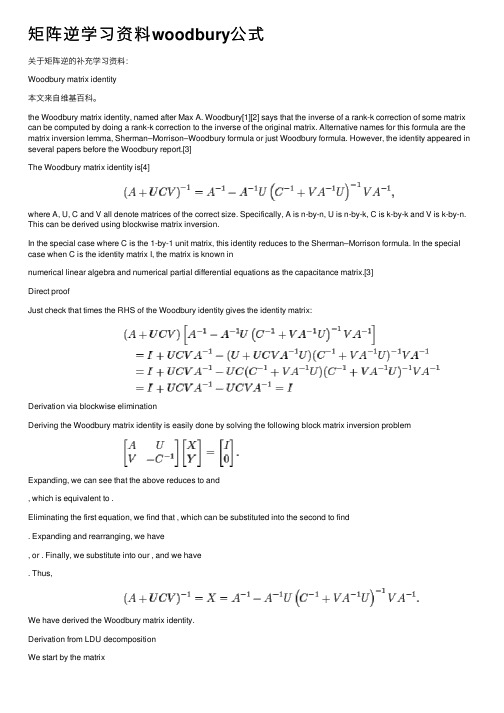
the Woodbury matrix identity, named after Max A. Woodbury[1][2] says that the inverse of a rank-k correction of some matrix can be computed by doing a rank-k correction to the inverse of the original matrix. Alternative names for this formula are the matrix inversion lemma, Sherman–Morrison–Woodbury formula or just Woodbury formula. However, the identity appeared in several papers before the Woodbury report.[3]The Woodbury matrix identity is[4]where A, U, C and V all denote matrices of the correct size. Specifically, A is n-by-n, U is n-by-k, C is k-by-k and V is k-by-n. This can be derived using blockwise matrix inversion.In the special case where C is the 1-by-1 unit matrix, this identity reduces to the Sherman–Morrison formula. In the special case when C is the identity matrix I, the matrix is known innumerical linear algebra and numerical partial differential equations as the capacitance matrix.[3]Direct proofJust check that times the RHS of the Woodbury identity gives the identity matrix:Derivation via blockwise eliminationDeriving the Woodbury matrix identity is easily done by solving the following block matrix inversion problemExpanding, we can see that the above reduces to and, which is equivalent to .Eliminating the first equation, we find that , which can be substituted into the second to find. Expanding and rearranging, we have, or . Finally, we substitute into our , and we have. Thus,We have derived the Woodbury matrix identity.Derivation from LDU decompositionWe start by the matrixBy eliminating the entry under the A (given that A is invertible) we getLikewise, eliminating the entry above C givesNow combining the above two, we getMoving to the right side giveswhich is the LDU decomposition of the block matrix into an upper triangular, diagonal, and lower triangular matrices.Now inverting both sides givesWe could equally well have done it the other way (provided that C is invertible) i.e.Now again inverting both sides,Now comparing elements (1,1) of the RHS of (1) and (2) above gives the Woodbury formulaApplicationsThis identity is useful in certain numerical computations where A?1has already been computed and it is desired to compute (A+ UCV)?1. With the inverse of A available, it is only necessary tofind the inverse of C?1+ VA?1U in order to obtain the result using the right-hand side of the identity. If C has a much smaller dimension than A, this is more efficient than inverting A+ UCV directly. A common case is finding the inverse of a low-rank update A+ UCV of A (where U only has a few columns and V only a few rows), or finding an approximation of the inverse of the matrix A+ B where the matrix can be approximated by a low-rank matrix UCV, for example using the singular value decomposition.This is applied, e.g., in the Kalman filter and recursive least squares methods, to replace the parametric solution, requiring inversion of a state vector sized matrix, with a condition equations based solution. In case of the Kalman filter this matrix has the dimensions of the vector of observations, i.e., as small as 1 in case only one new observation is processed at a time. This significantly speeds up the often real time calculations of the filter.See also：Sherman–Morrison formulaInvertible matrixSchur complementMatrix determinant lemma, formula for a rank-k update to a determinantBinomial inverse theorem; slightly more general identity. Notes：1.Jump up ^ Max A. Woodbury, Inverting modified matrices, MemorandumRept. 42, Statistical Research Group, Princeton University,Princeton, NJ, 1950, 4pp MR381362.Jump up ^ Max A. Woodbury, The Stability of Out-Input Matrices.Chicago, Ill., 1949. 5 pp. MR325643.^ Jump up to: a b Hager, William W. (1989). "Updating the inverse of amatrix". SIAM Review31 (2): 221–239. doi:10.1137/1031049.JSTOR2030425. MR997457.4.Jump up ^Higham, Nicholas (2002). Accuracy and Stability ofNumerical Algorithms (2nd ed.). SIAM. p. 258. ISBN978-0-89871-521-7. MR1927606.Press, WH; Teukolsky, SA; Vetterling, WT; Flannery, BP (2007), "Section 2.7.3. Woodbury Formula", Numerical Recipes: The Artof Scientific Computing (3rd ed.), New York: CambridgeUniversity Press, ISBN978-0-521-88068-8External links：Some matrix identitiesWeisstein, Eric W., "Woodbury formula", MathWorld.src="///doc/2742834010661ed9ad51f3e6.html /wiki/Special:CentralAutoLogin/start?type=1x1" alt="" title="" width="1" height="1" style="border: none; position: absolute;" />Retrieved from"/doc/2742834010661ed9ad51f3e6.html /w/index.php?title=Woodbury_matrix_identity&oldid=627695139"Categories:Linear algebraLemmasSherman–Morrison formula（来⾃维基百科。

[转载]图的拉普拉斯矩阵学习-Laplacian

[转载]图的拉普拉斯矩阵学习-Laplacian Matrices of Graphs We all learn one way of solving linear equations when we first encounter linearalgebra: Gaussian Elimination. In this survey, I will tell the story of some remarkable connections between algorithms, spectral graph theory, functional analysisand numerical linear algebra that arise in the search for asymptotically faster algorithms.I will only consider the problem of solving systems of linear equationsin the Laplacian matrices of graphs. This is a very special case, but it is also avery interesting case. I begin by introducing the main characters in the story.1. Laplacian Matrices and Graphs. We will consider weighted, undirected,simple graphs G given by a triple (V,E,w), where V is a set of vertices, Eis a set of edges, and w is a weight function that assigns a positive weight toevery edge. The Laplacian matrix L of a graph is most naturally defined bythe quadratic form it induces. For a vector x ∈ IRV , the Laplacian quadraticform of G is：Thus, L provides a measure of the smoothness of x over the edges in G. Themore x jumps over an edge, the larger the quadratic form becomes.The Laplacian L also has a simple description as a matrix. Define theweighted degree of a vertex u by：Define D to be the diagonal matrix whose diagonal contains d, and definethe weighted adjacency matrix of G by:We haveL = D − A.It is often convenient to consider the normalized Laplacian of a graph insteadof the Laplacian. It is given by D−1/2LD−1/2, and is more closely related tothe behavior of random walks.Regression on Graphs. Imagine that you have been told the value of afunction f on a subset W of the vertices of G, and wish to estimate thevalues of f at the remaining vertices. Of course, this is not possible unlessf respects the graph structure in some way. One reasonable assumption isthat the quadratic form in the Laplacian is small, in which case one mayestimate f by solving for the function f : V → IR minimizing f TLf subjectto f taking the given values on W (see [ZGL03]). Alternatively, one couldassume that the value of f at every vertex v is the weighted average of f atthe neighbors of v, with the weights being proportional to the edge weights.In this case, one should minimize:|D-1Lf|subject to f taking the given values on W. These problems inspire manyuses of graph Laplacians in Machine Learning.。

Introduction to Linear Algebra

»a = 5 a= 5
A vector is a mathematical quantity that is completely described by its magnitude and direction. An example of a three dimensional column vector might be 4 b= 3 5 uld easily assign bT to another variable c, as follows:
»c = b' c= 4 3 5
A matrix is a rectangular array of scalars, or in some instances, algebraic expressions which evaluate to scalars. Matrices are said to be m by n, where m is the number of rows in the matrix and n is the number of columns. A 3 by 4 matrix is shown here 2 A= 7 5 5 3 2 3 2 0 6 1 3 (3)
»a = 5;
Here we have used the semicolon operator to suppress the echo of the result. Without this semicolon MATLAB would display the result of the assignment:
»A(2,4) ans = 1
The transpose operator “flips” a matrix along its diagonal elements, creating a new matrix with the ith row being equal to the jth column of the original matrix, e.g. T A = 2 5 3 6 7 3 2 1 5 2 0 3

Matrix Derivative_wiki

Matrix calculusIn mathematics, matrix calculus is a specialized notation for doing multivariable calculus, especially over spaces of matrices, where it defines the matrix derivative. This notation was to describe systems of differential equations, and taking derivatives of matrix-valued functions with respect to matrix variables. This notation is commonly used in statistics and engineering, while the tensor index notation is preferred in physics.NoticeThis article uses another definition for vector and matrix calculus than the form often encountered within the field of estimation theory and pattern recognition. The resulting equations will therefore appear to be transposed when compared to the equations used in textbooks within these fields.NotationLet M(n,m) denote the space of real n×m matrices with n rows and m columns, such matrices will be denoted using bold capital letters: A, X, Y, etc. An element of M(n,1), that is, a column vector, is denoted with a boldface lowercase letter: a, x, y, etc. An element of M(1,1) is a scalar, denoted with lowercase italic typeface: a, t, x, etc. X T denotes matrix transpose, tr(X) is trace, and det(X) is the determinant. All functions are assumed to be of differentiability class C1 unless otherwise noted. Generally letters from first half of the alphabet (a, b, c, …) will be used to denote constants, and from the second half (t, x, y, …) to denote variables.Vector calculusBecause the space M(n,1) is identified with the Euclidean space R n and M(1,1) is identified with R, the notations developed here can accommodate the usual operations of vector calculus.•The tangent vector to a curve x : R→ R n is•The gradient of a scalar function f : R n→ RThe directional derivative of f in the direction of v is then•The pushforward or differential of a function f : R m→ R n is described by the Jacobian matrix The pushforward along f of a vector v in R m isMatrix calculusFor the purposes of defining derivatives of simple functions, not much changes with matrix spaces; the space of n×m matrices is isomorphic to the vector space R nm. The three derivatives familiar from vector calculus have close analogues here, though beware the complications that arise in the identities below.•The tangent vector of a curve F : R→ M(n,m)•The gradient of a scalar function f : M(n,m) → RNotice that the indexing of the gradient with respect to X is transposed as compared with the indexing of X. The directional derivative of f in the direction of matrix Y is given by•The differential or the matrix derivative of a function F : M(n,m) → M(p,q) is an element of M(p,q) ⊗ M(m,n), a fourth-rank tensor (the reversal of m and n here indicates the dual space of M(n,m)). In short it is an m×n matrix each of whose entries is a p×q matrix.is a p×q matrix defined as above. Note also that this matrix has its indexing and note that each ∂F/∂Xi,jtransposed; m rows and n columns. The pushforward along F of an n×m matrix Y in M(n,m) is thenas formal block matrices.Note that this definition encompasses all of the preceding definitions as special cases.According to Jan R. Magnus and Heinz Neudecker, the following notations are both unsuitable, as the determinants of the resulting matrices would have "no interpretation" and "a useful chain rule does not exist" if these notations are being used:[1]1.2.The Jacobian matrix, according to Magnus and Neudecker,[1] isIdentitiesNote that matrix multiplication is not commutative, so in these identities, the order must not be changed.•Chain rule: If Z is a function of Y which in turn is a function of X, and these are all column vectors, then•Product rule:In all cases where the derivatives do not involve tensor products (for example, Y has more than one row and X has more than one column),ExamplesDerivative of linear functionsThis section lists some commonly used vector derivative formulas for linear equations evaluating to a vector.Derivative of quadratic functionsThis section lists some commonly used vector derivative formulas for quadratic matrix equations evaluating to a scalar.Related to this is the derivative of the Euclidean norm:Derivative of matrix tracesThis section shows examples of matrix differentiation of common trace equations.Derivative of matrix determinantRelation to other derivativesThe matrix derivative is a convenient notation for keeping track of partial derivatives for doing calculations. The Fréchet derivative is the standard way in the setting of functional analysis to take derivatives with respect to vectors. In the case that a matrix function of a matrix is Fréchet differentiable, the two derivatives will agree up to translation of notations. As is the case in general for partial derivatives, some formulae may extend under weaker analytic conditions than the existence of the derivative as approximating linear mapping.UsagesMatrix calculus is used for deriving optimal stochastic estimators, often involving the use of Lagrange multipliers. This includes the derivation of:•Kalman filter•Wiener filter•Expectation-maximization algorithm for Gaussian mixtureAlternativesThe tensor index notation with its Einstein summation convention is very similar to the matrix calculus, except one writes only a single component at a time. It has the advantage that one can easily manipulate arbitrarily high rank tensors, whereas tensors of rank higher than two are quite unwieldy with matrix notation. Note that a matrix can be considered simply a tensor of rank two.Notes[1]Magnus, Jan R.; Neudecker, Heinz (1999 (1988)). Matrix Differential Calculus. Wiley Series in Probability and Statistics (revised ed.).Wiley. pp. 171–173.External links•Matrix Calculus (/engineering/cas/courses.d/IFEM.d/IFEM.AppD.d/IFEM.AppD.pdf) appendix from Introduction to Finite Element Methods book on University of Colorado at Boulder.Uses the Hessian (transpose to Jacobian) definition of vector and matrix derivatives.•Matrix calculus (/hp/staff/dmb/matrix/calculus.html) Matrix Reference Manual , Imperial College London.•The Matrix Cookbook (), with a derivatives chapter. Uses the Hessian definition.Article Sources and Contributors5Article Sources and ContributorsMatrix calculus Source: /w/index.php?oldid=408981406 Contributors: Ahmadabdolkader, Albmont, Altenmann, Arthur Rubin, Ashigabou, AugPi, Blaisorblade,Bloodshedder, CBM, Charles Matthews, Cooli46, Cs32en, Ctacmo, DJ Clayworth, DRHagen, Dattorro, Dimarudoy, Dlohcierekim, Enisbayramoglu, Eroblar, Esoth, Excirial, Fred Bauder,Freddy2222, Gauge, Geometry guy, Giftlite, Giro720, Guohonghao, Hu12, Immunize, Jan mei118, Jitse Niesen, Lethe, Michael Hardy, MrOllie, NawlinWiki, Oli Filth, Orderud, Oussjarrouse, Ozob, Pearle, RJFJR, Rich Farmbrough, SDC, Sanchan89, Stpasha, TStein, The Thing That Should Not Be, Vgmddg, Willking1979, Xiaodi.Hou, Yuzisee, 170 anonymous editsLicenseCreative Commons Attribution-Share Alike 3.0 Unported/licenses/by-sa/3.0/。

中山大学计算机学院离散数学基础教学大纲(2019)

中山大学本科教学大纲Undergraduate Course Syllabus学院（系）：数据科学与计算机学院School (Department)：School of Data and Computer Science课程名称：离散数学基础Course Title：Discrete Mathematics二〇二〇年离散数学教学大纲Course Syllabus: Discreate Mathematics（编写日期：2020 年12 月）(Date: 19/12/2020)一、课程基本说明I. Basic Information二、课程基本内容 II. Course Content（一）课程内容i. Course Content1、逻辑与证明（22学时） Logic and Proofs (22 hours)1.1 命题逻辑的语法和语义(4学时) Propositional Logic (4 hours)命题的概念、命题逻辑联结词和复合命题，命题的真值表和命题运算的优先级，自然语言命题的符号化Propositional Logic, logic operators (negation, conjunction, disjunction, implication, bicondition), compound propositions, truth table, translating sentences into logic expressions1.2 命题公式等值演算(2学时) Logical Equivalences (2 hours)命题之间的关系、逻辑等值和逻辑蕴含，基本等值式，等值演算Logical equivalence, basic laws of logical equivalences, constructing new logical equivalences1.3 命题逻辑的推理理论（2学时）论断模式，论断的有效性及其证明，推理规则，命题逻辑中的基本推理规则（假言推理、假言易位、假言三段论、析取三段论、附加律、化简律、合取律）,构造推理有效性的形式证明方法Argument forms, validity of arguments, inference rules, formal proofs1.4 谓词逻辑的语法和语义 (4学时) Predicates and Quantifiers (4 hours)命题逻辑的局限，个体与谓词、量词、全程量词与存在量词，自由变量与约束变量，谓词公式的真值，带量词的自然语言命题的符号化Limitations of propositional logic, individuals and predicates, quantifiers, the universal quantification and conjunction, the existential quantification and disjunction, free variables and bound variables, logic equivalences involving quantifiers, translating sentences into quantified expressions.1.4 谓词公式等值演算(2学时) Nested Quantifiers (2 hours)谓词公式之间的逻辑蕴含与逻辑等值，带嵌套量词的自然语言命题的符号化，嵌套量词与逻辑等值Understanding statements involving nested quantifiers, the order of quantifiers, translating sentences into logical expressions involving nested quantifiers, logical equivalences involving nested quantifiers.1.5谓词逻辑的推理规则和有效推理(4学时) Rules of Inference (4 hours)证明的基本含和证明的形式结构，带量词公式的推理规则（全程量词实例化、全程量词一般化、存在量词实例化、存在量词一般化），证明的构造Arguments, argument forms, validity of arguments, rules of inference for propositional logic (modus ponens, modus tollens, hypothetical syllogism, disjunctive syllogism, addition, simplication, conjunction), using rules of inference to build arguments, rules of inference for quantified statements (universal instantiation, universal generalization, existential instantiation, existential generalization)1.6 数学证明简介(2学时) Introduction to Proofs (2 hours)数学证明的相关术语、直接证明、通过逆反命题证明、反证法、证明中常见的错误Terminology of proofs, direct proofs, proof by contraposition, proof by contradiction, mistakes in proofs1.7 数学证明方法与策略初步(2学时) Proof Methods and Strategy (2 hours)穷举法、分情况证明、存在命题的证明、证明策略（前向与后向推理）Exhaustive proof, proof by cases, existence proofs, proof strategies (forward and backward reasoning)2、集合、函数和关系（18学时）Sets, Functions and Relations(18 hours)2.1 集合及其运算(3学时) Sets (3 hours)集合与元素、集合的表示、集合相等、文氏图、子集、幂集、笛卡尔积Set and its elements, set representations, set identities, Venn diagrams, subsets, power sets, Cartesian products.集合基本运算（并、交、补）、广义并与广义交、集合基本恒等式Unions, intersections, differences, complements, generalized unions and intersections, basic laws for set identities.2.2函数(3学时) Functions (3 hours)函数的定义、域和共域、像和原像、函数相等、单函数与满函数、函数逆与函数复合、函数图像Functions, domains and codomains, images and pre-images, function identity, one-to-one and onto functions, inverse functions and compositions of functions.2.3. 集合的基数（1学时）集合等势、有穷集、无穷集、可数集和不可数集Set equinumerous, finite set, infinite set, countable set, uncountable set.2.4 集合的归纳定义、归纳法和递归（3学时）Inductive sets, inductions and recursions (3 hours)自然数的归纳定义，自然数上的归纳法和递归函数；数学归纳法（第一数学归纳法）及应用举例、强归纳法（第二数学归纳法）及应用举例；集合一般归纳定义模式、结构归纳法和递归函数。

matrix_cookbook

The Matrix Cookbook
Kaare Brandt Petersen Michael Syskind Pedersen Version: October 3, 2005
What is this? These pages are a collection of facts (identities, approximations, inequalities, relations, ...) about matrices and matters relating to them. It is collected in this form for the convenience of anyone who wants a quick desktop reference . Disclaimer: The identities, approximations and relations presented here were obviously not invented but collected, borrowed and copied from a large amount of sources. These sources include similar but shorter notes found on the internet and appendices in books - see the references for a full list. Errors: Very likely there are errors, typos, and mistakes for which we apologize and would be grateful to receive corrections at cookbook@2302.dk. Its ongoing: The project of keeping a large repository of relations involving matrices is naturally ongoing and the version will be apparent from the date in the header. Suggestions: Your suggestion for additional content or elaboration of some topics is most welcome at cookbook@2302.dk. Acknowledgements: We would like to thank the following for discussions, proofreading, extensive corrections and suggestions: Esben Hoegh-Rasmussen and Vasile Sima. Keywords: Matrix algebra, matrix relations, matrix identities, derivative of determinant, derivative of inverse matrix, diﬀerentiate a matrix.

1、下载文档前请自行甄别文档内容的完整性，平台不提供额外的编辑、内容补充、找答案等附加服务。
2、"仅部分预览"的文档,不可在线预览部分如存在完整性等问题,可反馈申请退款(可完整预览的文档不适用该条件!)。
3、如文档侵犯您的权益，请联系客服反馈,我们会尽快为您处理(人工客服工作时间：9:00-18:30)。

1 1 1 2 2 4 5 9 12
1 1 2 3 3 32 1 4 = 33 , 3 1 5 34 9 4 1 . . .. . . . . . ···
where the ﬁrst column sequence A002212 in [13], which has two interpretations, the number of 3-Motzkin paths or the number of ways to assemble benzene rings into a tree [8]. Recall that a 3-Motzkin path is a lattice path from (0, 0) to (n−1, 0) that does not go below the x-axis and consists of up steps U = (1, 1), down steps D = (1, −1), and three types of horizontal steps H = (1, 0). The above matrix A = (ai,j ) is generated by the ﬁrst column and the following recurrence relation ai,j = ai−1,j −1 + 3ai−1,j + ai−1,j +1 . We may prove the above identities (1.5) and (1.6) by using method of Riordan arrays. So the natural question is to ﬁnd a matrix identity for the sequence (1, k, k 2 , k 3 , . . .). We need the combinatorial interpretation of the entries in the matrix in terms of weighted partial Motzkin paths, as given by Cameron and Nkwanta [4]. To be precise, a partial Motzkin path, also called a Motzkin path from (0, 0) to (n, k ) in [4], is just a Motzkin path but without the requirement of ending on the x-axis. A weighted partial Motkzin a partial Motzkin path with the weight assignment that the horizontal steps are endowed with a weight k and the down steps are endowed with a weight t, where k and t are regarded as positive integers. In this sense, our weighted Motzkin paths can be regarded as further generalization of k -Motzkin paths in the sense of 2-Motzkin paths and 3-Motkzin paths [1, 7, 13]. We introduce the notion of weighted free Motzkin paths which is a lattice path consisting of Motzkin steps without the restrictions that it has to end with a point on the x-axis and it does not go below the x-axis. We then give a bijection between weighted free Motzkin paths and weighted partial Motzkin paths with an elevation line, which leads to a matrix identity involving the number of weighted partial Motzkin paths and the sequence (1, k, k 2 , . . .). The idea of the elevation operation is also used by Cameron and Nkwanta in their combinatorial proof of the identity (1.1) in a more restricted form. By extending our argument to weighted partial Motzkin paths with multiple elevation lines, we obtain a combinatorial proof of an identity recently derived by Cameron and Nkwanta, in answer to their question. We also give a generalization of the matrix identity (1.1) and give a combinatorial proof by using colored Dyck paths.
Matrix Identities on Weighted Partial Motzkin Paths
arXiv:math/0509255v1 [math.CO] 12 Sep 2005
William Y.C. Chen1 , Nelson Y. Li2 , Louis W. Shapiro3 and Sherry H. F. Yan4
(1.5)
where the ﬁrst column is the sequence of Motzkin numbers, and matrix A = (aij ) is generated by the following recurrence relation: ai,j = ai−1,j −1 + ai−1,j + ai−1,j 1 chen@, 2 nelsonli@, 3 lshapiro@,
Abstract. We give a combinatorial interpretation of a matrix identity on Catalan numbers and the sequence (1, 4, 42, 43 , . . .) which has been derived by Shapiro, Woan and Getu by using Riordan arrays. By giving a bijection between weighted partial Motzkin paths with an elevation line and weighted free Motzkin paths, we ﬁnd a matrix identity on the number of weighted Motzkin paths and the sequence (1, k, k 2 , k 3 , . . .) for any k ≥ 2. By extending this argument to partial Motzkin paths with multiple elevation lines, we give a combinatorial proof of an identity recently obtained by Cameron and Nkwanta. A matrix identity on colored Dyck paths is also given, leading to a matrix identity for the sequence (1, t2 + t, (t2 + t)2 , . . .). Key words: Catalan number, Schr¨ oder number, Dyck path, Motzkin path, partial Motzkin path, free Motzkin path, weighted Motzkin path, Riordan array AMS Mathematical Subject Classifications: 05A15, 05A19. Corresponding Author: William Y. C. Chen, chen@
for j ≥ 2 and the ai,1 is the i-th little Schr¨ oder number si (sequence A001003 in [13]), which counts Schr¨ oder paths of length 2(i + 1). A Schr¨ oder path is a lattice path starting at (0, 0) and ending at (2n, 0) and using steps H = (2, 0), U = (1, 1) and D = (1, −1) such that no steps are below the x-axis and there are no peaks at level one. Imposing this last peak condition gives us little Schr¨ oder numbers while without it we would have the large Schr¨ oder numbers. For k = 3, we obtain the following matrix identity on Motzkin numbers: