Computing the lattice of all fixpoints of a fuzzy closure operator
庞加莱 关于数学创造(翻译)

庞加莱关于数学创造(翻译)庞加莱关于数学创造(翻译)2010-11-15 15:37:21昨天刘未鹏在日志中提到庞加莱关于数学创造的文章,顺手译成了中文,如下:Mathematical Creation数学创造How is mathematics made? What sort of brain is it that can compose the propositions and systems of mathematics? How do the mental processes of the geometer or algebraist compare with those of the musician, the poet,the painter, the chess player? In mathematical creation which are the key elements? Intuition? An exquisite sense of space and time? The precision of a calculating machine?A powerful memory? Formidable skill in following complex logical sequences? A supreme capacity for concentration? 数学是由什么构成的?哪种类型的大脑能够创造数学的定理和系统?几何学家或是代数学家的思维活动和音乐家、是人画家和象棋选手有什么不同?数学创造中,哪些是关键元素?直觉?空间和时间的精确感觉?机器一般的计算准确性?超强的记忆力?复杂逻辑推导的超强技能?极好的注意力?The essay below, delivered in the first years of this century as a lecture before the Psychological Society in Paris, is the most celebrated of the attempts to describe what goes on in the mathematician's brain. Its author, Henri Poincaré, cousin of Raymond, the politician, was peculiarly fitted to undertake the task. One of the foremost mathematicians of all time, unrivaled as an analyst and mathematical physicist, Poincaré was known also as a brilliantly lucid expositor of the philosophy of science. These writings are of the first importance as professional treatises for scientists and are at the same time accessible, in large part, to the understanding of the thoughtful layman.下面的文章,是本世纪(20世纪)初期在巴黎心理学会上做的一次报告,是描述关于数学家大脑如何运转的最著名的尝试。
有效质量 英语

有效质量英语Effective MassThe concept of effective mass is a fundamental principle in physics that has far-reaching implications in various fields, from semiconductor technology to particle physics. Effective mass is a crucial parameter that describes the behavior of particles, particularly in the context of their interaction with external forces or fields.At its core, effective mass is a measure of the "apparent" or "effective" mass of a particle, which can differ from its actual or rest mass. This difference arises due to the complex interactions between the particle and its surrounding environment, such as the potential energy fields or the crystal structure of a material.In the case of a free particle, such as an electron in a vacuum, its effective mass is equal to its rest mass. However, when a particle is subjected to a potential energy field or is embedded within a material, its effective mass can deviate significantly from its rest mass. This phenomenon is particularly evident in semiconductor materials, where the effective mass of charge carriers (electrons and holes) plays a crucial role in determining the material's electronic andoptical properties.In semiconductor materials, the periodic potential created by the crystal lattice can significantly modify the effective mass of charge carriers. This modification is a result of the complex interactions between the charge carriers and the periodic potential, which can be described using the principles of quantum mechanics.The effective mass of charge carriers in semiconductors is a key parameter that determines the mobility, conductivity, and other important characteristics of the material. For example, in the design of electronic devices such as transistors and integrated circuits, the effective mass of charge carriers is a critical factor in optimizing device performance and efficiency.Moreover, the concept of effective mass extends beyond the realm of semiconductor physics. In particle physics, the effective mass of particles, such as subatomic particles or quasiparticles, is crucial for understanding their behavior and interactions within complex systems. For instance, the effective mass of particles in high-energy physics experiments can provide insights into the fundamental nature of matter and the forces that govern the universe.One of the most fascinating aspects of effective mass is its ability to exhibit exotic and counterintuitive behavior. In certain materials, suchas graphene or topological insulators, the charge carriers can exhibit an effective mass that is negative or even diverges to infinity. These unusual effective mass properties can lead to the emergence of novel physical phenomena, such as the quantum Hall effect or the formation of Dirac or Weyl fermions.The study of effective mass has also been instrumental in the development of cutting-edge technologies, such as quantum computing and spintronics. In these fields, the manipulation and control of the effective mass of charge carriers or spin-polarized particles are crucial for the realization of advanced devices and the exploration of quantum mechanical effects.In conclusion, the concept of effective mass is a fundamental principle in physics that has far-reaching implications across various disciplines. From semiconductor technology to particle physics, the effective mass of particles plays a vital role in understanding and predicting the behavior of complex systems. As scientific research continues to push the boundaries of our understanding, the study of effective mass will undoubtedly remain a crucial area of investigation, with the potential to unlock new frontiers in our quest to unravel the mysteries of the physical world.。
Exact algorithms for the minimum latency problem

Exact algorithms for the minimum latency problemBang Ye Wu∗,Zheng-Nan Huang,Fu-Jie ZhanDept.of Computer Science and Information Engineering,Shu-Te University,YenChau,Kaohsiung,Taiwan824,R.O.C.Key words:algorithms,minimum latency problem,dynamic programming,branch and bound1IntroductionLet G=(V,E,w)be an undirected graph with positive weight w(e)on each edge e∈E. Given a starting vertex s∈V and a subset U⊂V as the demand vertex set,the minimum latency problem(MLP)asks for a tour P starting at s and visiting each demand vertex at least once such that the total latency of all demand vertices is minimized,in which the latency of a vertex is the length of the path from s to thefirst visit of the vertex.The MLP is an important problem in computer science and operations research,and is also known as the delivery man problem or the traveling repairman problem.Similar to the well-known traveling salesperson problem(TSP),in the MLP we are asked tofind an“optimal”way for routing a server passing through the demand vertices.The difference is the objective functions.The latency of a vertex can be thought of as the delay of the service.In the MLP we care about the total delay(service quality),while the total length(service cost)is concerned in the TSP.The MLP on a metric space is NP-hard and also MAX-SNP-hard[4].Polynomial time algorithms are only known for very special graphs,such as paths[1,6],edge-unweighted trees[9],trees of diameter3[4],trees of constant number of leaves[8],or graphs with similar structure[12].Even for caterpillars(paths with edges sticking out),no polynomial time algorithm has been reported.In a recent work,it is shown that the MLP on edge-weighted trees is NP-hard[11].Due to the NP-hardness,many works ∗corresponding author(bangye@.tw)have been devoted to the approximation algorithms[2,3,4,7,8],and the current best approximation ratio is3.59[5].More references to exact and approximation algorithms can be found in those papers.“Dynamic programming”(DP)and“branch-and-bound”(B&B)are two popular strate-gies used to exactly solve NP-hard problems without exhaustive search.As pointed out in [12],the MLP can be exactly solved by a dynamic programming algorithm.However,the algorithm is still very time-consuming.By designing non-trivial lower bound functions and using a technique combining the advantages of both DP and B&B,we developed a series of exact algorithms for the MLP.Experimental results on both random and real data are also reported in this paper.The results show that our algorithm is much more efficient than the DP algorithm and the B&B algorithm,and we believe that the technique can be also applied to some other problems.2PreliminariesIn this paper,a graph is a simple and connected graph with a nonnegative weight on each edge.Throughout this paper,the input graph is G,and n is the number of nodes of graph G.An origin(starting vertex)is a given vertex of G.A tour is a route from the origin and visiting each vertex at least once.A subtour is a partial or a complete tour starting at the origin.Let H be a subgraph or a subtour.The set of vertices of H is denoted by V(H).For u,v∈V(G),we use d G(u,v)to denote the length of the shortest path between u and v on G.For a subtour P,d P(u,v)denotes the distance from thefirst visit of u to thefirst visit of v in P,and w(P)denotes the length of P.Definition1:Let P be a subtour starting at s on graph G.For a demand vertex v visited by P,the latency of v is defined as d P(s,v),which is the distance from the origin to thefirstvisit of v on P.The latency of a tour P is defined by L(P)=v∈Ud P(s,v),in which U isthe demand vertex set.In general,the input graph of a MLP may be any simple connected graph with nonnegative edge weights,and the demand vertex set does not necessarily include all the vertices.Ametric graph is a complete graph with edge weights satisfying the triangle inequality.By a simple reduction,we may assume that the input graph is always a metric graph and all the vertices are the demand vertices.Let G=(V,E,w)be the underlying graph and U⊂V be the demand vertex set.Wefirst compute the metric closure¯G=(U,U×U,¯w)of G,in which the weight on each edge is the shortest path length of the two endpoints in G.For any tour ¯P on¯G,we can construct a corresponding tour P on G by simply replacing each edge in¯P with the corresponding shortest path on G.It is easy to see that L(P)≤L(¯P).Conversely, given any tour P on G,we can obtain a tour¯P on¯G by eliminating all vertices not in U. Since the edge weight is the shortest path length,we have L(¯P)≤L(P).Consequently the minimum latencies of the two graphs are the same.Furthermore,if there exists an O(T(n)) time exact or approximation algorithm for the MLP on metric graphs,the MLP on general graphs can be solved in O(T(n)+f(n))time with the same performance guarantee,in which f(n)is the time complexity for computing the all-pairs shortest path length.In the remaining paragraphs,we assume that the input graph G is a metric graph and each vertex is a demand vertex.It should also be noted that the optimal tour never visits the same vertex twice in a metric graph.3Algorithms3.1Pure dynamic programmingTofind the optimal tour of a MLP,a brute force algorithm checking all permutations of the vertices except for the origin will takeΩ((n−1)!)time.In[12],it was pointed out that the MLP can be solved in O(n22n)time by a dynamic programming algorithm.For the completeness,we briefly explain the algorithm in the following.Definition2:Let P be a subtour on graph G.Define a cost function c(P)=L(P)+ (n−|V(P)|)w(P),i.e.,c(P)is the total latency of the visited vertices plus the length of P multiplied by the number of vertices not been visited.Let P1and P0be two routes such that the last vertex of P1is thefirst vertex of P0.We use P1//P0to denote the route obtained by concatenating P1and P0.For a subtour P,we say that P has configuration(R,v),in which R=V(P)and v is the last vertex of P. The dynamic programming algorithm is based on the following property which can be easily shown by definition.It also explains the reason why we define the cost function c in such a way.Claim1:Let P1and P2be subtours with the same configuration and c(P1)≤c(P2).If Y2=P2//P0is a complete tour,i.e.,P0is a route starting at the last vertex of P2and visiting all the remaining vertices,then Y1=P1//P0is also a tour and L(Y1)≤L(Y2).Tofind the minimum latency,by Claim1,we only need to keep one subtour for each possible configuration.The dynamic programming algorithm starts at the subtour containing only the origin and computes the best subtour for each configuration in the order that the number of the visited vertex is from small to large.The time complexity then follows that there are O(n2n)configurations and we generate O(n)subtours when a subtour is extended by one vertex.3.2Dynamic programming with pruningTo make the program more efficient,we introduce a pruning technique in the DP algorithm, which is similar to the one used in a typical branch-and-bound algorithm.While the program is running,we always record an upper bound(UB)of the optimal,which is the latency of some feasible tour.For each generated subtour P,we compute a lower bound of P,which is an under estimate of any complete tour containing P as a prefix.If the lower bound of a subtour is no less than UB,we can prune the subtour without affecting the optimality of the final solution.The key points are how we compute the UB and how we estimate the lower bound of a subtour.A pure DP algorithm does not generate any complete tour until it reaches the configura-tions consisting of the set of all vertices.To get an upper bound,we employ a simple greedy algorithm to build a tour.The greedy algorithm uses the“nearest vertexfirst”strategy. Beginning with a subtour containing only the origin,we repeatedly augment the subtour by one vertex until all vertices are included.At each iteration,we choose the vertex which isnearest to the stopping vertex of the subtour and has not been visited.Obviously,such a tour can be computed in O(n2)time.In addition to the initial stage,our algorithm uses the greedy method to build a tour whenever a new subtour is generated,and keep the current best solution.Algorithm DPwP MLPInput:A metric graph G=(V,E,w)and an origin s∈V.Output:The latency of the optimal tour.//Q i is a queue for storing the generated subtours consisting of i vertices.1:Initiate Q1,and insert subtour(s)into Q1.2:Get an upper bound UB of the optimal.3:For i←1to n−1do4:For each subtour P in Q i do5:compute an upper bound UB from P;6:if UB <UB7:UB←UB ;8:For each vertex v not in V(P)do9:generate a subtour P =P//(v);10:if there exists a subtour with the same configuration in Q i+111:keep the one with better c(·)value;12:else13:compute a lower bound LB of P ;14:if LB<UB then insert P into Q i+1;15:Output UB as the minimum latency.At Step10,we need to search a configuration in Q i+1.In a typical DP algorithm, such a step can be implemented by employing an array,of which each element is for one configuration.By suitably encoding the configurations,the search can be done in only one memory access.However,such a simple method is not suitable for our algorithm since it requires to check every configuration,and this is what we want to avoid.Because of the large size of the queue,a good data structure should be used.In our program,we use an AVL tree.In the next section,we shall present the experimental results,and it shows that the improvement is very significant,compared to a link list implementation.As in a typical B&B algorithm,the lower bound function is a key point to the efficiency of the algorithm.The running time depends heavily on two factors:the number of the generated subtours and the time to compute a lower bound of a subtour.A lower bound function eliminating many subtours may be bad if it suffers from a long computation time.In the following,let G=(V,E,w)be the input metric graph and s be the origin.Let P be a subtour stopping at a vertex r and Y=P//P0be the best tour consisting of P as its prefix. Let¯V=V−V(P),¯n=|¯V|,and P0=(v0=r,v1,v2...,v¯n).Remember that the best tour never visits a vertex twice in a metric graph.A function is a LB function of P if the latency of Y is lower bounded by the value of the function.We begin with a simple observation.For any1≤i≤¯n,by the triangle inequality,we haved Y(s,v i)=w(P)+d Y(r,v i)≥w(P)+w(r,v i).Therefore,L(Y)≥L(P)+¯ni=1(w(P)+w(r,v i))=L(P)+¯n w(P)+¯ni=1w(r,v i)=c(P)+v∈¯Vw(r,v). The following property is obvious,and we omit the proof.Claim2:The function B1(P)=c(P)+v∈¯Vw(r,v)is a LB function of P and can becomputed in O(n)time.Next,we generalize the simple idea.Let l i(r,v)be the length of the shortest i-edges path between vertices r and v.Thereby an i-edges path is a path consisting of exactly i different edges.Wefirst show the following property.Lemma3:For any vertices r and v,l i(r,v)≤l j(r,v)if i<j.Proof:It is sufficient to show that l i(r,v)≤l i+1(r,v).Let Q=(r,u1,u2,...,u i+1=v) be the shortest(i+1)-edges path.Then Q =(r,u2,...,u i+1)is an i-edges path,and w(Q )≤w(Q)since w(r,u2)≤w(r,u1)+w(u1,u2)by the triangle inequality.By the definition of li,we have l i(r,v)≤w(Q ),and this completes the proof.Note that l1(r,v)is exactly w(r,v)by definition.By the monotonic property of l i,it is natural to use a more general l i as the lower bound function.In the next theorem,we establish a family of lower bound functions.Note that the function B1coincides with the one in Claim 2.Theorem4:Let k≥1.The functionB k(P)=c(P)+v∈¯V l k(r,v)−k−1i=1maxv∈¯V{l k(r,v)−l i(r,v)}is a LB function of P and can be computed in O(kn)time if the value l i(r,v)is available for any1≤i≤k and any v∈¯V.Proof:Clearly l i(r,v i)≤d Y(r,v i)since d Y(r,v i)is the length of an i-edges path while l i(r,v i)is the minimum among all possible such paths.Furthermore,by Lemma3,we have l i(r,v)≤d Y(r,v j)for any j≥i,and therefore,for k≥1,L(Y)=c(P)+¯ni=1d Y(r,v i)≥c(P)+¯ni=1l i(r,v i)≥c(P)+k−1i=1l i(r,v i)+¯ni=kl k(r,v i)(1)For i<k,we rewritel i(r,v i)=l k(r,v i)−(l k(r,v i)−l i(r,v i)) in Eq.(1),and obtainL(Y)≥c(P)+¯ni=1l k(r,v i)−k−1i=1(l k(r,v i)−l i(r,v i))≥c(P)+v∈¯V l k(r,v)−k−1i=1maxv∈¯V{l k(r,v)−l i(r,v)}Finally the time complexity is obviously O(kn).Although it is very time-consuming to compute l k even for small k,we compute the values only once in a preprocessing stage.As a subtour is generated,we need only O(kn)time to obtain a lower bound.We summarize the time complexity of the algorithm in the next theorem.Theorem5:The algorithm DPwP MLP with lower bound function B k runs in O(n k+1+ n2T)time,in which T is the number of generated subtours.Proof:To employ B k as the lower bound function,we compute l i(u,v)for any1≤i≤k and each vertex pair(u,v)in a preprocessing stage.Since l i(u,v)is the length of the shortest i-edges path and an i-edges path containing exactly i−1intermediate vertices,all these values can be computed in O(n k+1)time by exhaustively checking all possible permutations.For each generated subtour,at Step5–7,we compute a feasible tour and update the upper bound if necessary,and it takes O(n2)time.For searching the configuration in Q i+1at Step 10,by employing an AVL tree,we perform O(log|Q i+1|)comparisons of configurations.Since there are at most n2n configurations,the number of comparisons is O(n).A configuration consists of a vertex and a set of up to n paring two configurations takes O(n) time.Therefore,the total time for searching the AVL trees is O(n2T),in which T is the total number of generated subtours.For Step13,by Theorem4,the time for computing the lower bounds of all subtours is O(knT).For Step14,since inserting an element into the AVL tree has the same time complexity as the searching,the total time for all the insertions is also O(n2T).In summary, the time complexity of the algorithm is therefore O(n k+1+n2T).4The experimental resultsWe implemented the algorithms in C language and investigated their practical performances. All the tests were performed on personal computers,each of which is equipped with an Intel Pentium IV2.4GHz CPU and256M bytes memory.Two types of test data were used: random data and real data.For each test case,the running time includes all the steps except for generating or calculating the input distances.4.1Random dataThe random data were generated artificially with edge weights drawn from uniform distribu-tion.All the edge weights are integers between1and1024.In Table1,we summarize the maximum running time for each program in the tests on random data.Algorithm DPP(i) denote the algorithm DPwP MLP with lower bound function B i.For the sake of compari-Table1:The maximum running time in the random data tests(seconds,K=1000)BF10.5K165K-------DP 1.45 3.278.3817.740.096.812.5K*--DPP L 1.07 2.7725.299.4367 4.07K8.41K--DPP(1)0.300.50 2.03 4.1911.343.781.018011.7K* DPP(2)0.220.38 1.44 2.947.6629.154.6166302 DPP(3)0.170.280.91 2.03 5.2717.737.2128247 DPP(4)0.250.47 1.00 2.06 4.9111.125.896.6176 DPP(5) 1.45 2.56 4.928.0313.722.740.5105165B&B(1) 1.80 3.9115.055.7161 1.77K 2.97K 6.50K-Table2:The maximum number of generated subtours in random data tests(M=106)n=18 1.1M0.23M0.12M0.11M789896985514.8M n=2110.5M 2.96M 1.99M 1.32M0.83M0.51M593M n=23-9.17M7.35M 6.51M 4.51M 3.26M-son,we also implemented the brute-force method(labeled by BF)and the branch-and-bound method(labeled by B&B(1),using the lower bound function B1).The BF computes the op-timal solution by simply checking all the possible permutations.The B&B(1)program is similar to DPP(1)except that it does not merge the subtours with the same configuration. It uses the depth-first strategy to choose the subtour to be extended,and the chosen subtour is augmented by each of the vertices not been visited yet.In fact,we also implemented the branch-and-bound method with B i,i>1.But their behaviors are similar,and we only list B&B(1)for comparison.Algorithm DPP L is the same as DPP(1)but using a link list instead of an AVL tree as the data structure for storing the configurations.Basically at least one hundred data instances were used for each problem size.But,for BF and DP,only few instances are tested because their performances almost do not vary with the input data of the same number of vertices.Some cells in the table are marked with “-”to indicate that we did not complete the tests on these cases because some data instances took too long to complete.A“*”in a cell indicates that the long running time is caused by“disk swap”in the virtual memory system.In Table2,we list the maximum number of subtours generated by each program for some typical values of n.Table3:The running time in the real data tests(seconds)Ulysses160.090.080.090.130.330.45 Ulysses22 3.40 3.53 3.50 3.42 5.5554.47 Gr2454.4751.5443.6434.4130.23285.17 Fri2639.6137.6432.7526.0927.41257.60 4.2Real dataIn addition to the random data,we also used real data to test the performances of the algorithms.The data instances are chosen from TSPLIB[10]for the sake of their problem sizes.The results are shown in Table3.Note that the number appeared in the name indicates the number of vertices for each instance.In fact,we have also performed some other tests on partial data drawn from larger instances in TSPLIB.The results are similar.Roughly speaking,problems with25–26vertices can be solved in paring with the results of random data,the performances are much better.The reason may be that the real data are more structured and therefore the bad cases rarely happen.5Discussion and concluding remarksBy the experimental results and some other observations in our development,we make the following conclusions.•The algorithm DPwP MLP takes the advantages of both the dynamic programming and the branch-and-bound strategies,and significantly improves the performance.•Using a good data structure such as the AVL tree in our program is very important.The reason is obvious by knowing the numbers of the generated subtours(Table2).•For small integers j>i,DPP(j)is better than DPP(i)when n exceeds some value.•Theoretically,we can improve the lower bound by restricting that the i-edge path can only visit the vertices in¯V.But it suffers from a long computation time and therefore has a worse performance.In fact,we have tried several other lower bound functions.Some of them eliminate much more subtours than B1but has a worse performance.References[1]F.Afrati,S.Cosmadakis,C.Papadimitriou,G.Papageorgiou,and N.Papakostantinou,The complexity of the traveling repairman problem,Theoretical Informatics and Appli-cations,20(1)(1986)79–87.[2]A.Archer and D.P.Williamson,Faster approximation algorithms for the minimum la-tency problem,in Proc.14th ACM-SIAM Symposium on Discrete Algorithms(SODA 2003),2003pp.88–96.[3]S.Arora and G.Karakostas,Approximation schemes for minimum latency problems,SIAM put.,32(5)(2003)1317-1337.[4]A.Blum,P.Chalasani,D.Coppersmith,B.Pulleyblank,P.Raghavan,and M.Sudan,Theminimum latency problem,in Proc.26th ACM Symposium on the Theory of Computing (STOC’94),1994pp.163–171.[5]K.Chaudhuri,B.Godfrey,S.Rao,and K.Talwar,Paths,Trees,and Minimum LatencyTours,in Proc.44th Symposium on Foundations of Computer Science(FOCS2003),2003 pp.36–45.[6]A.Garcia,P.Jodr´a,and J.Tejel,A note on the traveling repairmen problem,Networks,40(1)(2002)27–31.[7]M.Goemans and J.Kleinberg,An improved approximation ratio for the minimum latencyproblem,Math.Program.,82(1998)114–124.[8]E.Koutsoupias,C.Papadimitriou and M.Yannakakis,Searching afixed graph,in Proc.23nd Colloquium on Automata,Languages and Programming,Lecture Notes in Comput.Sci.,Vol.1099,1996,pp.280–289.[9]E.Minieka,The delivery man problem on a tree network,Ann.Oper.Res.,18(1989)261–266.[10]G.Reinelt,TSPLIB—a traveling salesman problem library,ORSA puting,3(1991)376–384.See also http://www.iwr.uni-heidelberg.de/groups/comopt/software-/tsplib95/.[11]R.Sitters,The minimum latency problem is NP-hard for weighted trees,in Proc.9thInternational IPCO Conference,Lecture Notes in Comput.Sci.,Vol.2337,2002,pp.230–239.[12]B.Y.Wu,Polynomial time algorithms for some minimum latency problems,Inf.Process.Lett.,75(5)(2000)225–229.11。
算法导论 第三版 第22章 答案 英

Michelle Bodnar, Andrew Lohr April 12, 2016
Exercise 22.1-1 Since it seems as though the list for the neighbors of each vertex v is just an undecorated list, to find the length of each would take time O(out − degree(v )). So, the total cost will be v∈V O(outdegree(v )) = O(|E | + |V |). Note that the |V | showing up in the asymptotics is necessary, because it still takes a constant amount of time to know that a list is empty. This time could be reduced to O(|V |) if for each list in the adjacency list representation, we just also stored its length. To compute the in degree of each vertex, we will have to scan through all of the adjacency lists and keep counters for how many times each vertex has appeared. As in the previous case, the time to scan through all of the adjacency lists takes time O(|E | + |V |). Exercise 22.1-2 The adjacency list representation: 1 : 2, 3 2 : 1, 4, 5 3 : 1, 6, 7 4:2 5:5 6:3 7 : 3.
铝的晶格常数-体弹模量及弹性常数分子模拟

铝的晶格常数-体弹模量及弹性常数分子模拟CCCalculation of material lattice constant and bulk modulus 2012 Calculation of materiallatticeconstantand bulk modulusSummary :Aluminum is one of the world's most used metals, the calculated aluminum lattice constant and bulk modulus can be used to improve the performance of the aluminum consequently make better use of aluminum. In virtue of molecular dynamics simulation software ,we can solve the lattice constant . By the derivative of the lattice con s tant, the bulk modulus can be obtained. The elastic constants of a material display the elasticity and we can use the software material studio to simulate and get them. The simulation results match the experimental values. Key words:Aluminum, lattice constant, bulk modulus, elastic constant , simulation.Introduction:In materials science, in order to facilitate analysis about the way in which the crystal particles are arranged, the basic unit can be removed from the crystal lattice as a representative (usually the smallest parallel hexahedron) as a compositionunit of dot matrix, called a cell (i.e. solid State Physics "original cell" concept); lattice constant (or so-called lattice constant) refers to the side length of the unit cell, in other words, the side length of each parallel hexahedral cells. Lattice constant is an important basic parameters of crystal structure. Figure A is the basic form of the lattice constant.Figure ALattice constant is a basic structural parameter,which has a direct relationship with the bondings between the atoms ,of the crystal substance. It reflects the changes in the internal composition of the crystal of the lattice constant, force state changes, etc.The bulk modulus (K or B) of a substance measures thesubstance's resistance touniform compression. It isdefined as the ratio of theinfinitesimal pressure increaseto the resulting relative decreaseof the volume. Its base unit is thepascal. Figure B describes theeffect of bulk modulus.Figure BThe bulk modulus canbe formally defined by theequation:where is pressure, isvolume, and denotes thederivative of pressure withrespect to volume.Our research object isaluminum,whose atomicnumber is 13 and relative massis 27.The reserves of aluminumranks only second to ferrumcompared with other metallicelements. Aluminum andaluminum alloy are consideredthe most economic andapplicable in many applicationfields as a consequence of theirexcellent properties. What’smore,increased usage ofaluminum will result fromdesigners' increased familiaritywith the metal and solution tomanufacturing problems thatlimit some applications.The crystal structure of aluminum is face-centered cubic. The experimental value of lattice constant and bulk modulus are 0.0.40491nm and 79.2Gpa. Computing theory and methods:Our simulation is on the basis that aluminum is offace-centered cubic crystal structure. We can get the exact value of lattice constant in virtue of molecular dynamics simulation software. Then by the derivation of lattice constant for energy E,we obtain bulk modulus.To start with ,compile a script for the use of operation and simulation in lammps. We set periodicboundary conditions in the script and create an analog box,whose x ,y ,z coordinate values are all confined to [0,3].Run the script in lammps, calculating the potential energy,kinetic energy as well as the nearest neighbor atoms for each atom. Finally put out the potential energy function of aluminum.Extract the datas under the linux system produced by lammps to continue the computation by means of matlab,from which we can get the lattice constant through several times of matching.Figure CFigure C——the curve shows the relationship between cohesive energy and lattice constant,which is what we get in the process of computing in matlab,points out the lattice constant corresponding with the least cohesive energy. The horizontal ordinate of the rock bottom stand for the lattice constant of aluminum which can be clearly located as 0.40500nm.Since we have obtained the lattice constant,we simulated the visualization of aluminu’s crystal structure. Figure D is what we get through the visualization.Figure DThe bulk modulus is defined as:As for cubic cell,the formula can be transformed into the following pattern:The bulk modulus can be calculated with the formula above combined with the latticeconstant. Finally,the bulk modulus is 78.1Gpa.Besides,to enrich our research, we have calculated the elastic constants of aluminum. Because of the symmetry of face-centered cubic,aluminum only has three elastic constants. To reach the target ,we have to establish a cell of aluminum in the software material studio in the first place and then transform it into a primitive cell. Figure E and figure F are the cell and the primitive cell we have established during the simulation .Figure EFigure FIt comes to the CASTEP step after the geometry optimization. We managed to makeE cut=350eV andK points=16*16*16 ,both of which are extremely importantand also sensitive to the calculation of elastic constant,after several trials. Figure G is the primitive cell that has been through the geometry optimization.Figure GThe calculated results are as follows:C11=106.2GpaC12=60.5GpaC44=28.7Gpa Correspondingly ,the experimental range of the three elastic constants are listed below:C11=108~112GpaC12=61.3~66GpaC44=27.9~28.5GpaAs we can see,although a little outside of the value range of the experimental standards, our results are right within the error range.Conclusion:Our group has calculated the lattice constant and bulk modulus of aluminum,both of which coincide with the experimental value,by means of lammps and matlab. Moreover ,we have found out that bulk modulus has a close relationshipwith temperature. As lattice constant haven’t made any change under small change of temperature while the energy of the material have changed,so we concluded that temperature change can influence bulk modulus as a consequence of the change of cohesive energy change resulting from temperature change.There are still problems in our research as you can see that the three elastic constants are a little out of the value range. But this group is the one closest to the experimental value. Our group have concluded that the errors result from the script which can affect the accuracy of the simulation.Besides,the most valuable thing we have learned is that we must seek the solutions and never give up in face of difficulties.References:[1]材料科学基础(胡赓祥、蔡珣、戎咏华上海交通大学出版社)[2]Ayton, Gary; Smondyrev, Alexander M; Bardenhagen, Scott G; McMurtry, Patrick; Voth, Gregory A.“Calculating the bulk modulus for a lipid bilayer with none quilibrium molecular dynamics simulation". Biophysical Society. 2002.[3]Cohen, Marvin (1985).CCCalculation of material lattice constant and bulk modulus 2012 "Calculation of bulk modulus ofdiamond and zinc-blende solids". Phys. Rev. B 32: 7988–7991. [4] Watson, I G; Lee, P D; Dashwood, R J; Young, P . Simulation of the Mechanical Properties of an Aluminum Matrix Composite using X-ray Microtomography: Physical Metallurgical and Materials Science. Springer Science & Business Media. 2006. [6] Ashley, Steven. Aluminum vehicle breaks new ground. Engineering--Mechanical Engineering. Feb 1994. [7] Sanders, Robert E, Jr; Farnsworth, David M. Trends in Aluminum Materials Usage forElectronics. Metallurgy. Oct2011.附文:lammps脚本units metalboundary p p patom_style atomicvariable i loop 20variable x equal 4.0+0.01*$ilattice fcc $xregion box block 0 3 0 3 0 3 create_box 1 boxcreate_atoms 1 boxpair_style adppair_coeff * * AlCu.adp Almass 1 27neighbor 1 binneigh_modify every 1 delay 5 check yes variable p equal pe/108variable r equal 108/($x*3)^3 timestep 0.005thermo 10compute 3 all pe/atomcompute 4 all ke/atomcompute 5 all coord/atom 3dump 1 all custom 100 dump.atom id xs ys zs c_3 c_4 c_5dump_modify 1format"%d %16.9g %16.9g %16.9g%16.9g %16.9g %g"min_style sdminimize 1.0e-12 1.0e-12 1000 1000print "@@@@ (latticeparameter,rho,energy per atom):$x$r $p"clearnext ijump in.al至于代码的含义,可参考其它资料或查询lammps官网manual。
Lecture14_Lattice_Structures
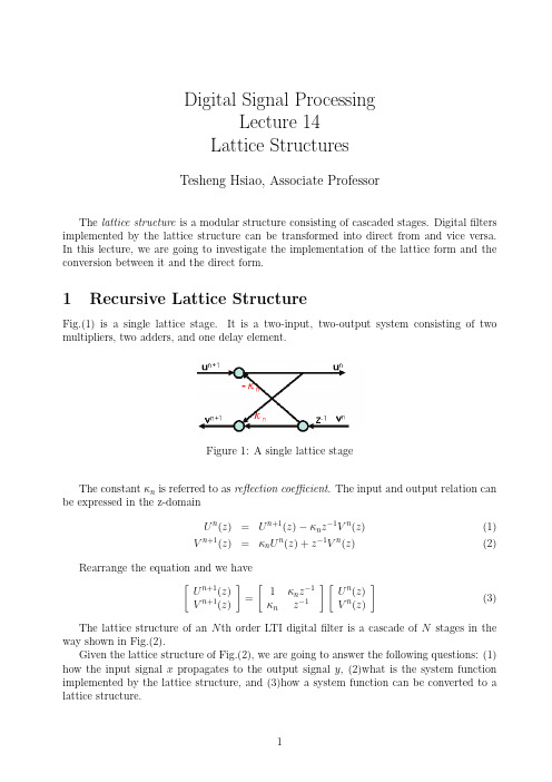
Digital Signal ProcessingLecture 14Lattice StructuresTesheng Hsiao,Associate ProfessorThe lattice structure is a modular structure consisting of cascaded stages.Digital filters implemented by the lattice structure can be transformed into direct from and vice versa.In this lecture,we are going to investigate the implementation of the lattice form and the conversion between it and the direct form.1Recursive Lattice StructureFig.(1)is a single lattice stage.It is a two-input,two-output system consisting of two multipliers,two adders,and one delayelement.Figure 1:A single lattice stageThe constant κn is referred to as reflection coefficient .The input and output relation can be expressed in the z-domainU n (z )=U n +1(z )−κn z −1V n (z )(1)V n +1(z )=κn U n (z )+z −1V n (z )(2)Rearrange the equation and we have[U n +1(z )V n +1(z )]=[1κn z −1κn z −1][U n (z )V n (z )](3)The lattice structure of an N th order LTI digital filter is a cascade of N stages in the way shown in Fig.(2).Given the lattice structure of Fig.(2),we are going to answer the following questions:(1)how the input signal x propagates to the output signal y ,(2)what is the system function implemented by the lattice structure,and (3)how a system function can be converted to a lattice structure.Figure2:Recursive lattice structure•Lattice FilteringThe output of the lattice structure can be calculated in a recursive way.Assume that the system is at initial rest;hence v n[−1]=0,n=0,1,···,N−1.From Fig.(2),for each time step k≥0,we haveinitial conditions:v n[−1]=0,n=0,1,···,N−1for k=0,1,2,···u N[k]=x[k]for n=N−1to0u n[k]=u n+1[k]−κn v n[k−1]v n+1[k]=κn u n[k]+v n[k−1]endv0[k]=u0[k]y[k]=N∑n=0λn v n[k]end•The system function of the lattice structureLetP n(z)=U n(z)U0(z),Q n(z)=V n(z)V0(z),n=0,1,2,···,NHence,Eq.(3)can be rewritten as[P n+1(z) Q n+1(z)]=[1κn z−1κn z−1][P n(z)Q n(z)],n=0,1,2,···,N−1(4) =[1κnκn1][P n(z)z−1Q n(z)],n=0,1,2,···,N−1(5)Note thatU0(z)=V0(z),P0(z)=Q0(z)=1,X(z)U0(z)=P N(z),Y(z)U0(z)=N∑n=0λn Q n(z)Therefore the system function H (z )isH (z )=Y (z )X (z )=∑N n =0λn Q n (z )P N (z )(6)If we expand Eq.(4),we obtain [P n (z )Q n (z )]=[1κn −1z −1κn −1z −1]···[1κ0z −1κ0z −1][11],n =0,1,···,N (7)It is clear from Eq.(7)that P n (z )and Q n (z )are polynomials of z −1of order n .From Eq.(6),P N (z )is the denominator of H (z )while ∑N n =0λn Q n (z )is the numerator ofH (z ).Note that the number of parameters in the lattice structure (κn ,n =0,···N −1and λn ,n =0,···,N )is the same as the number of coefficients of an N th order rational function.In summary,the system function H (z )can be determined by applying Eq.(4)recur-sively to find P n (z )and Q n (z ),n =1,2,···,N ,given Q 0(z )=P 0(z )=1.Then use Eq.(6)to determine H (z ).•Convert the direct form to the lattice structureLet P n (z )=p n 0+p n 1z −1+···+p n n z−n and Q n (z )=q n 0+q n 1z −1+···+q n n z −n ;From Eq.(7),we have [P 1(z )Q 1(z )]=[1κ0z −1κ0z −1][11]=[1+κ0z −1κ0+z −1][P 2(z )Q 2(z )]=[1κ1z −1κ1z −1][1+κ0z −1κ0+z −1]=[1+(κ0+κ0κ1)z −1+κ1z −2κ1+(κ1κ0+κ0)z −1+z −2]...=...Hence we conclude by induction that p n n =κn −1and q n n =1for n =0,1,2,···,N .Moreover we have the following lemma.Lemma 1Q n (z )=z −n P n (z −1),n =0,1,···,NProof:This lemma can be proved by induction.The n =0case is trivialFor n =1,P 1(z )=1+κ0z −1and Q 1(z )=κ0+z −1.Thus the equality holds.Suppose that the equality holds for n =k ,i.e.Q k (z )=z −k P k (z −1).Equivalently,z −k Q k (z −1)=P k (z )For n =k +1,from Eq.(4)we haveP k +1(z )=P k (z )+κk z −1Q k (z )Q k +1(z )=κk P k (z )+z −1Q k (z )Thereforez −(k +1)P k +1(z −1)=z −k −1P k (z −1)+κk z −k Q k (z −1)=z −1Q k (z )+κk P k (z )=Q k +1(z )Thus,by mathematical induction Q n (z )=z −n P n (z −1)for n =0,1,···,NQ.E.D.Assume that κn =1for all n .If we inverse Eq.(5),we have[P n (z )z −1Q n (z )]=11−κ2n[1−κn −κn 1][P n +1(z )Q n +1(z )],n =0,1,···,N −1Hence,P n(z )=P n +1(z )−κn Q n +1(z )1−κ2n ,n =N −1,N −2,···,0(8)Let H (z )=B (z )A (z )=∑N n =0b n z −n 1−∑N n =1a n z −n ,where A (z )andB (z )are polynomials of z −1.Since p n n =κn −1for all n ,thereflection coefficients κn ’s can be determined recur-sively by first setting P N (z )=A (z )and Q N (z )=z −N P N (z −1).Then κN −1=p N N is determined.Applying Eq.(8)and Lemma 1recursively to find P n (z ),κn ’s can be determined successively.To determine λn ,we observe that the coefficient of z −N in the numerator must beλN since B (z )=∑Nn =0λn Q n (z )and q N N =1.Therefore λN =b N .We can removeλN Q N (z )from B (z ),resulting in a (N −1)th order polynomial,and determine λN −1by taking advantage of the property q n n =1for all n .The whole process continuous until all λn ’s are determined.In summaryP N =A (z ),S N =B (z ),λN =b Nfor n =N −1to 0κn =p n +1n +1Q n +1(z )=z −(n +1)P n +1(z −1)P n (z )=P n +1(z )−κn Q n +1(z )1−κ2nS n (z )=S n +1(z )−λn +1Q n +1(z )λn =s n nend•Stability of the Lattice Structure Form Eq.(4),we haveP 1(z )=1+κ0z −111is stable if and only if |κ0|<1.Since the lattice structure is a cascade of N similar stages,the stability of the filter can be verified easily as follows.Lemma 2The lattice structure in Fig.(2)is stable if and only if |κn |<1for all n .2All-pole SystemsAn all-pole system has no nonzero zeros,i.e.the system function is H (z )=1A (z ).In thelattice structure in Fig.(2),if λ0=1and λn =0for n >0,thenH (z )=∑N n =0λn Q n (z )P N (z )=1P N (z )Hence the all-pole system has a simpler lattice structure shown in Fig.(3).Figure 3:The lattice Structure for an all-pole systemOne interesting feature of the lattice structure in Fig.(3)is that the system function from x to v N is an all-pass system.This can be seen as follows.H all (z )=V N (z )X (z )=Q N (z )P N (z )=z −N P N (z −1)P N (z )If z 0is a pole of H all (z ),then 1/z 0must be a zero of H all (z )and vice versa.Due to the symmetry of poles and zeros,H all (z )is indeed an all-pass system.3Nonrecursive lattice structureIf H (z )=B (z ),i.e an FIR filter,the lattice structure becomes nonrecursive.We will explore its properties in this section.We would like to maintain the symmetric structure in Fig.(2)or Fig.(3)because previous results (e.q.Lemma 1)can be applied directly by doing so.In other words,Eq.(1)and Eq.(2)must hold for each stage.If H (z )is FIR,then G (z )=H −1(z )is an all-pole system.If we implement the all-pole system G (z )in the lattice form of Fig.(3),we haveG (z )=1H (z )=1P N (z )=U 0(z )U N (z )By exchanging its input and output,we get the desired FIR system.Note that in this FIR lattice structure,signals flow from u 0to u N .Hence Eq.(3)should be used to compute the signal propagation from stage to stage.The corresponding lattice structure is shown in Fig.(4).Notice that the structure is nonrecursive.The system function implemented by the nonrecursive lattice structure can be constructed in the same way as the recursive lattice structure:P 0(z )=Q 0(z )=1for n =1to N [P n (z )Q n (z )]=[1κn −1z −1κn −1z −1][P n −1(z )Q n −1(z )]endH(z)=P N(z)Figure4:Nonrecursive Lattice StructureTo convert from a system function to the nonrecursive lattice structure,the algorithm is similar to that of the recursive version:P N=B(z)=1+b1z−1+···+b N z−Nfor n=N to1κn−1=p nnQ n(z)=z−n P n(z−1)P n−1(z)=P n(z)−κn−1Q n(z)1−κ2n−1endNote that from Lemma1,p n0=q nn=1for all n.Therefore the coefficient of the constantterm in H(z),i.e.b0,must be1.If b0=1,an intuitive approach is to divide B(z)by b0. However,if b N=b0,as in the case of the linear phasefilter,this will result inκN−1=1, and again we will run into trouble in computing the reflection coefficients.A preferable way is to implement the FIR system H′(z)=1+(B(z)−b0)in a lattice structure and subtract 1−b0from its output.The idea is shown in Fig.(5)Figure5:Nonrecursive lattice structure for b0=1If we apply Lemma2to the nonrecursive lattice structure,we observe that B(z)is a minimum phase system if and only if|κn|<1for all n.If B(z)=P N(z)is a minimum phase system,then the system function from x=u0to v N,i.e.Q N(z),becomes a maximum phase system according to Lemma1,i.e.all its zeros are outside the unit circle.Afinal remark of this lecture:According to Lemma2,each stage of the stable(or minimum phase)lattice structure is an attenuator,i.e.it does not amplify the signals.Thisproperty gives the lattice structure great computational stability and this is the primary reason that the lattice structure is implemented.However,the price for this property is the complex computation of the signalflow.。
Abstract Computing the Closest Point to a Circle

Computing the Closest Point to a CirclePinaki MitraNIMC,AliporeCalcutta,Indiae-mail:pinaki m@Asish Mukhopadhyay∗School of Computer Science University of Windsor,Windsor,Canada e-mail:asishm@uwindsor.caS.V.RaoDepartment of Computer Science&Engineering Indian Institute of Technology,Guwahati,India e-mail:svrao@iitg.ernet.inAbstractIn this paper we consider the problem of computing theclosest point to the boundary of a circle among a setS of n points.We present two algorithms to solve this problem.One algorithm runs in O(n3)prepro-cessing time and space and O(log2n)query time.The other algorithm runs in O(n1+ )preprocessing time and O(n log n)space and O(n2/3+ )query time.Thus we ex-hibit a trade-offbetween preprocessing and query times For dimensions d≥3we present an algorithm with O(n d/2 + )preprocessing time to report an approx-imate closest point to the boundary of d-dimensional query sphere R in O(n1−1/(d+1)+ )query time.1IntroductionThe problem of preprocessing a set S,of n points in the plane to determine the closest point to a query line was initially addressed by Cole and Yap[2],who obtained a solution with preprocessing time and space in O(n2)and query time in O(log n).Lee and Ching[6]obtained the same result using geometric duality.In[8]an algorithm was presented with O(n log n)preprocessing time and space and O(n0.695)query time.The space complexity was improved to O(n)in a subsequent result by Mi-tra and Chaudhuri[9].In[10],the simplicial partition technique of[7]was used to improve the query time to O(n1/2+ )for arbitrary >0,with preprocessing time and space in O(n1+ )and O(n log n)respectively.In this paper,we consider a natural extension of the above problem-determining a point in S that is closest to the boundary of a query circle.Ourfirst algorithm precomputes all higher order Voronoi diagrams.The preprocessing time and space complexities of this algo-rithm are in O(n3),while the query time is in O(log2n). We propose another algorithm that uses the simplicial partition idea of Matousek[7].The preprocessing time and space complexities of this algorithm are in O(n1+ )∗Research supported by an NSERC Operating Grant and O(n log n)respectively,while the query time is in O(n2/3+ ).The second approach generalizes to higher dimen-sions.Here,however,point location turns out to be a bottleneck.Recently,some attempts have been made to overcome this problem by computing an approxi-mate nearest neighbor in higher dimensions[4].Tak-ing a cue from this,for dimension d≥3,we propose an algorithm thatfinds an approximate closest point, according to two different approximation schemes,with preprocessing time in O(n d/2 + )and query time in O(n1−1/(d+1)+ ).2Geometric Insight for High Preprocessing and Low Query AlgorithmIn a preprocessing step,we compute all higher order Voronoi diagrams.The cost of this is in O(n3)[11].The main idea of the query procedure is a binary search on the pre-computed higher-order Voronoi diagrams.Let the query circle have centre at p and radius a. Algorithm Query(R)pute the nearest neighbor of p from V or1(S)and check if its distance from p is less than a.If not, we report the nearest neighbor of p as the answer to the query since in this case all points of S lies outside or on the boundary of the circle R.Stop.pute the furthest neighbor of p from V or n(S)and check if its distance from p is greater than a.If not,we report the furthest neighbor as the answer to the query since in this case all points of S lies inside or on the boundary of the circle R.Stop.3.Perform a binary search within the interval(1...n).Compute n/2 -th nearest neighbor of pfrom V or n/2 and determine its distance from p.If it is equal to a this point is the answer to our query.If it is greater than a recurse in the interval1(1... n/2 ).Otherwise,if it is less than a recursein the interval n/2 ...n.Thus determine the k-th and(k+1)-th nearest neighbors s and t of p such that(dist(p,s)<a)and(dist(p,t)>a).4.For each of the the two points s and t determinedin Step III,we compute the absolute difference of their distance from p and a.The point having the least value of the absolute difference is the answer to our query.Thus we have the following theorem.Theorem1Given a set S of n points,the closest point from the boundary of a query circle R can be computed in O(log2n)time with O(n3)preprocessing time and space.In the next section,we propose an alternate algo-rithm based on the simplicial partition technique of Ma-tousek[7]to improve the preprocessing time.3Simplicial PartitionsA simplicial partition of S is a collection of pairsΨ(S)={(S1,t1),(S2,t2),...,(S r,t r)}(1) where the S i’s are mutually disjoint subsets of S whose union is S,and each t i is a tetrahedron that contains S i (see Fig.1).A simplicial partition isfine if|S i|≤2∗n/r for each i.For a given simplicial partitionΨ(S),the crossing number of a plane Q is the number of tetrahedrons of Ψ(S)that the plane properly intersects.The crossing number ofΨ(S)is the maximum crossing number over all planes that intersect the simplicial partition.The following theoretically important result by Ma-tousek[7]shows how to construct afine simplicial par-tition with a low crossing number.Theorem2For any given set S of n d-dimensional points and a parameter r,1≤r≤n,afine simplicial partition of size r,with O(r1−1/d)crossing number,ex-ists.Further,for any given >0,such a simplicial partition can be constructed in time O(n1+ ).Figure1:Plane Q cuts a simplicial partition.We lift the set S of n points and the query circle R,onto the surface of a paraboloid[3]z=x2+y2.S denotes the lifted set of points and R the plane through the image of the query circle.Points inside the circle R gets mapped to one halfspace and points outside the ring R gets mapped to the other halfspace.We construct afine simplicial partition of S of size r with crossing number O(r2/3).What is important for our problem is that each tetrahedron that is not intersected by R , traps a set of points whose projections lie completely inside or outside the query circle.We use the simplicial partition of the lifted set of points to create a r-way partition tree on the set of points S,keeping with each subset of points the corre-sponding tetrahedron that enclosed their lifted images in3-space.4Algorithmic DetailsThe constructibility of afine simplicial partition in3-space with a low crossing number implies that the pro-jections of the point sets enclosed by at least r−O(r2/3) simplices are not intersected by a query circle R.For the remaining at most O(r2/3)simplices that are inter-sected by S ,we proceed recursively on the respective partitions of the projections of the point sets enclosed by these tetrahedra.The preprocessing phase of the algorithm maintains both the nearest neighbor and furthest neighbor Voronoi diagrams of the point set corresponding to each node of the partition tree.Then preprocess each of the Voronoi diagram using the algorithm of Kirkpatrick[5]to per-form point location.Given a query circle R with center p and radius a, we answer the closest point query,using the following algorithm.Algorithm Q1.Initialize q to(∞,∞),the nearest point to the thequery ring.2.If the tetrahedron associated with the node of thepartition tree lies below R ,use the furthest neigh-bor Voronoi diagram of the projection of the point set inside the tetrahedron to detect the region in which the center p lies.Let t1be the point asso-ciated with this region.In Fig.2a,since p lies in V(p i)the closest point to the boundary of R is p i and thus t1=p i.If the absolute difference of the distance of t1from p and a is less than that of q update q to t1.3.If the tetrahedron associated with the node of thepartition tree lies above R ,use the nearest neigh-bor Voronoi diagram of the projection of the point set inside the quadrilateral to detect the region in2(b)(a)Figure 2:(a)Furthest neighbor Voronoi diagram is queried when the tetrahedron lies below R .(b)Nearest neighbor Voronoi diagram is queried when the tetrahe-dron lies above R .which the center p lies.Let t 2be the point asso-ciated with this region.In Fig.2b,since p lies in V (p j )the closest point to the boundary of R is p j and thus t 2=p j .If the absolute difference of the distance of t 2from p and a is less than that of q update q to t 2.4.If the tetrahedron associated with the node of the partition tree intersects R we recurse on the sub-trees rooted at that node of the partition tree.The complexity of the algorithm is summarized in the following theorem.Theorem 3Given a set S of n points and a query cir-cular circle R the closest point from the boundary of R in the set S can be answered in O (n 2/3+ )query time with O (n 1+ )preprocessing time and O (n log n )prepro-cessing space.The approach of the previous section extends to higher dimensions in exactly the same way.5Approximate nearest pointIf an approximate closest point is acceptable,we can avoid point location in higher dimensional Voronoi di-agrams required for an exact solution.We preprocess each partitioned point set using Clarkson’s [1]random-ized algorithm for the nearest neighbor query.For a set S of n points in d -dimension we can preprocess this setin O (n d/2 +)time to perform nearest neighbor query in O (log n )time.Now,for the furthest point query in the preprocessing phase we will maintain the furthest point from each point in the simplicial partition.For a partition with m points this computation can be easily done using any brute force algorithm in O (m 2)time in any dimension.Given a query sphere,if the whole par-tition lies completely inside,we will use the algorithm of Clarkson to compute the nearest neighbor q of the(a)(b)Figure 3:Diagram for the worst case:(a)first approxi-mation (b)second approximation.center p .Then use this furthest neighbor of q as an approximate furthest neighbor of p .Fig.3a illustrates the worst case situation if we adopt this approach.In this diagram we see that the actual furthest neighbor of p ,i.e.,t is at a distance which is almost 3times the distance of p from the reported fur-thest neighbor s .The constant of approximation can be improved if we increase the preprocessing overhead by maintaining the furthest neighbor of each data point in each of the 2d quadrants around that point.Again for a partition with m points this computation can be easily done using any brute force algorithm in O (m 2)time in any dimension.Now given the query circle we locate the nearest neigh-bor q of the center p .Then from O (2d )furthest points maintained for q we choose the one which is at maxi-mum distance from p .For fixed d thus we have to spend an additional O (1)time besides the O (log n )time near-est neighbor query.Fig.3b illustrates the worst case situation if we adopt this approach.In this diagram we see that the actual furthest neighbor of p ,i.e.,t is at a distance which is almost √5times the distance of p from the reported furthest neighbor s .Now if we try to bound the error of approximation from the boundary of the query sphere the error ratio is roughly (a −l/2− 1)/(a −kl/2+ 2),where k =3in the first approximation and k =√5in the second approximation.Thus for a >>l we have constant ap-proximation.But for values of a close to kl/2the error of approximation is high.The time complexity of preprocessing each partition using Clarkson’s algorithm [1]would dominate the time complexity of construction of the partition tree.Fol-lowing a similar analysis as done for two dimension,we establish the following theorem.Theorem 4Given a set of n points and a query sphere R in d dimensions,an approximate nearest neighbor from the boundary of the sphere can be computed inO (n 1−1/(d +1)+ )query time with O (n d/2 +)prepro-cessing.36ConclusionsIn this paper we have shown that the results of Mitra and Chaudhuri[9]can be generalized to answer the cir-cle query problem.We have presented two algorithms one with high preprocessing and low query time and the other one with low preprocessing and high query time. References[1]K.L.Clarkson.A randomized algorithm forclosest-point queries.SIAM put.,17:830–847,1988.[2]R.Cole and C.K.Yap.Geometric retrieval prob-lems.In Proc.24th Annu.IEEE Sympos.Found.Comput.Sci.,pages112–121,1983.[3]H.Edelsbrunner and R.Seidel.Voronoi diagramsand arrangements.Discrete Comput.Geom.,1:25–44,1986.[4]Piotr Indyk and Rajeev Motwani.Approximatenearest neighbors:Towards removing the curse of dimensionality.In Proc.30th Annu.ACM Sympos.Theory Comput.,page to appear,1998.[5]D.G.Kirkpatrick.Optimal search in planar sub-divisions.SIAM put.,12(1):28–35,1983. [6]D.T.Lee and Y.T.Ching.The power of geometricduality rm.Process.Lett.,21:117–122,1985.[7]J.Matouˇs ek.Efficient partition trees.DiscreteComput.Geom.,8:315–334,1992.[8]P.Mitra.Finding the closest point to a queryline.In G.Toussaint,editor,Snapshots in Compu-tational Geometry,volume II,pages53–63.1992.[9]P.Mitra and B.B.Chaudhuri.Efficiently com-puting the closest point to a query line.Pattern Recognition Letters,19:1027–1035,1998.[10]Asish ing simplicial paritions todetermine a closest point to a query line.Pattern Recognition Letters,24:1915–1920,2003.[11]F.P.Preparata and putationalGeometry:An Introduction.Springer-Verlag,3rd edition,October1990.4。
半导体物理与器件英语

半导体物理与器件英语Semiconductor Physics and DevicesThe field of semiconductor physics and devices is a crucial aspect of modern technology, as it underpins the development of a wide range of electronic devices and systems that have transformed our daily lives. Semiconductors, which are materials with electrical properties that lie between those of conductors and insulators, have been the backbone of the digital revolution, enabling the creation of integrated circuits, transistors, and other essential components found in smartphones, computers, and a myriad of other electronic devices.At the heart of semiconductor physics is the study of the behavior of electrons and holes within these materials. Electrons, which are negatively charged particles, and holes, which are the absence of electrons and carry a positive charge, are the fundamental charge carriers in semiconductors. The interactions and movement of these charge carriers within the semiconductor lattice structure are governed by the principles of quantum mechanics and solid-state physics.One of the fundamental concepts in semiconductor physics is theenergy band structure. Semiconductors have a unique energy band structure, with a filled valence band and an empty conduction band separated by an energy gap. The size of this energy gap determines the semiconductor's electrical properties, with materials having a smaller energy gap being more conductive than those with a larger gap.The ability to manipulate the energy band structure and the behavior of charge carriers in semiconductors has led to the development of a wide range of electronic devices. The most prominent of these is the transistor, a fundamental building block of modern electronics. Transistors are used to amplify or switch electronic signals and power, and they are the essential components in integrated circuits, which are the heart of digital devices such as computers, smartphones, and various other electronic systems.Another important class of semiconductor devices are diodes, which are two-terminal devices that allow the flow of current in only one direction. Diodes are used in a variety of applications, including power supplies, rectifiers, and light-emitting diodes (LEDs). LEDs, in particular, have become ubiquitous in modern lighting and display technologies, offering improved energy efficiency, longer lifespan, and enhanced color quality compared to traditional incandescent and fluorescent light sources.Semiconductor devices are not limited to electronic applications; they also play a crucial role in optoelectronics, a field that deals with the interaction between light and electronic devices. Photodetectors, such as photodiodes and phototransistors, are semiconductor devices that convert light into electrical signals, enabling a wide range of applications, including imaging, optical communication, and solar energy conversion.The development of semiconductor physics and devices has been a continuous process, driven by the relentless pursuit of improved performance, efficiency, and functionality. Over the past several decades, we have witnessed remarkable advancements in semiconductor technology, with the miniaturization of devices, the introduction of new materials, and the development of innovative device architectures.One of the most significant trends in semiconductor technology has been the scaling of transistor dimensions, often referred to as Moore's Law. This observation, made by Intel co-founder Gordon Moore in 1965, predicted that the number of transistors on a microchip would double approximately every two years, leading to a dramatic increase in computing power and a corresponding decrease in device size and cost.This scaling has been achieved through a combination ofadvancements in fabrication techniques, material engineering, and device design. For example, the use of high-k dielectric materials and the implementation of FinFET transistor architectures have allowed for continued scaling of transistor dimensions while maintaining or improving device performance and power efficiency.Beyond the scaling of individual devices, the integration of multiple semiconductor components on a single integrated circuit has led to the development of increasingly complex and capable electronic systems. System-on-a-chip (SoC) designs, which incorporate various functional blocks such as processors, memory, and input/output interfaces on a single semiconductor die, have become ubiquitous in modern electronic devices, enabling greater functionality, reduced power consumption, and improved overall system performance.The future of semiconductor physics and devices holds immense promise, with researchers and engineers exploring new materials, device architectures, and application domains. The emergence of wide-bandgap semiconductors, such as silicon carbide (SiC) and gallium nitride (GaN), has opened up new possibilities in high-power, high-frequency, and high-temperature electronics, enabling advancements in areas like electric vehicles, renewable energy systems, and communication networks.Additionally, the integration of semiconductor devices with otheremerging technologies, such as quantum computing, neuromorphic computing, and flexible/wearable electronics, is paving the way for even more transformative applications. These developments have the potential to revolutionize fields ranging from healthcare and transportation to energy and communication, ultimately enhancing our quality of life and shaping the technological landscape of the future.In conclusion, the field of semiconductor physics and devices is a cornerstone of modern technology, underpinning the development of a vast array of electronic devices and systems that have become indispensable in our daily lives. The continuous advancements in this field, driven by the relentless pursuit of improved performance, efficiency, and functionality, have been instrumental in driving the digital revolution and shaping the technological landscape of the21st century. As we move forward, the future of semiconductor physics and devices promises even more remarkable innovations and transformative applications that will continue to shape our world.。