matlab期末大作业
MATLAB期末大作业

MATLAB期末⼤作业学号:姓名:《Matlab/Simulink在数学计算与仿真中的应⽤》⼤作业1.假设地球和⽕星绕太阳运转的半径分别为r和2r,利⽤comet指令动画显⽰从地球到⽕星的转移轨迹(r可以任意取值,要求实时显⽰探测器、太阳、地球和⽕星的位置)。
解函数function comet(varargin)[ax,args,nargs] = axescheck(varargin{:});error(nargchk(1,3,nargs,'struct'));% Parse the rest of the inputsif nargs < 2, x = args{1}; y = x; x = 1:length(y); endif nargs == 2, [x,y] = deal(args{:}); endif nargs < 3, p = 0.10; endif nargs == 3, [x,y,p] = deal(args{:}); endif ~isscalar(p) || ~isreal(p) || p < 0 || p >= 1error('MATLAB:comet:InvalidP', ...'The input ''p'' must be a real scalar between 0 and 1.'); End指令 %particle_motiont = 0:5:16013;r1=6.7e6;%随便给定参数%---------------------------r2=2*r1;g=9.8;R=6.378e6;m=g*R^2;%内轨道v_inner=sqrt(m/r1);w_inner=v_inner/r1;x_inter=r1*cos(w_inner*t);y_inter=r1*sin(w_inner*t);%外轨道v_outer=sqrt(m/r2);w_outer=v_outer/r2;x_outer=r2*cos(w_outer*t);y_outer=r2*sin(w_outer*t);%控制器转移轨道a=(r1+r2)/2;E=-m/(2*a);V_near=sqrt(m*(2/r1-2/(r1+r2)));%转移轨道在近地点的速度V_far=sqrt(m*(2/r2-2/(r1+r2)));%转移轨道在远地点的速度h=r1*V_near;%由于在近地点的速度垂直于位置失量, h是转移轨道的⽐动量矩e=sqrt(1+2*E*h^2/m^2);%e为椭圆轨迹的偏⼼率TOF=pi*sqrt(a^3/m);%转移轨道是椭圆的⼀半及飞⾏时间是周期的⼀半(开普勒第三定律) w=pi/TOF;%椭圆轨迹的⾓速度c=a*e;b=sqrt(a^2-c^2);x_ellipse=a*cos(w*t)-0.5*r1;y_ellipse=b*sin(w*t);%动画显⽰运动轨迹x=[x_inter;x_outer;x_ellipse]';y=[y_inter;y_outer;y_ellipse]';comet(x,y)%---------------------------动态图像如下:2.利⽤两种不同途径求解边值问题dfdxf gdgdxf g f g=+=-+==34430001,,(),()的解.途径⼀:指令syms f g[f,g]=dsolve('Df=3*f+4*g,Dg=-4*f+3*g','f(0)=0,g(0)=1'); disp('f=');disp(f)disp('g=');disp(g)结果(Matlab 7.8版本)f=i/(2*exp(t*(4*i - 3))) - (i*exp(t*(4*i + 3)))/2g=exp(t*(4*i + 3))/2 + 1/(2*exp(t*(4*i - 3)))(Matlab 6.5版本)f=exp(3*t)*sin(4*t)g=exp(3*t)*cos(4*t)>>途径⼆:%problem2function dy=problem2(t,y)dy = zeros(2,1);dy(1) = 3*y(1)+4*y(2);dy(2) = -4*y(1)+3*y(2);[t,y] = ode45('problem2',[0 2],[0 1]);plot(t,y(:,1),'r',t,y(:,2),'b');图23.假设著名的Lorenz 模型的状态⽅程表⽰为-+-=+-=+-=)()()()()()()()()()()()(322133223211t x t x t x t x t x t x t x t x t x t x t x t x σρρβ其中,设28,10,3/8===σρβ。
[设计]《MATLAB语言及应用》期末大作业题目与解答
![[设计]《MATLAB语言及应用》期末大作业题目与解答](https://img.taocdn.com/s3/m/1394b362a517866fb84ae45c3b3567ec102ddc80.png)
《MATLAB语言及应用》期末大作业题目1.数组的创建和访问(20分,每小题2分):1)利用randn函数生成均值为1,方差为4的5*5矩阵A;2)将矩阵A按列拉长得到矩阵B;3)提取矩阵A的第2行、第3行、第2列和第4列元素组成2*2的矩阵C;4)寻找矩阵A中大于0的元素;]5)求矩阵A的转置矩阵D;6)对矩阵A进行上下对称交换后进行左右对称交换得到矩阵E;7)删除矩阵A的第2列和第4列得到矩阵F;8)求矩阵A的特政值和特征向量;9)求矩阵A的每一列的和值;10)求矩阵A的每一列的平均值;程序代码:clear;clc;A=1+sqrt(4)*randn(5) %生成均值为1,方差为4的5*5矩阵A;B=A(:) %将矩阵A按列拉长得到矩阵B;C=A([2 3],[2 4]) %提取矩阵A的第2行、第3行、第2列和第4列元素组成2*2的矩阵C;n=find(A>0) %寻找矩阵A中大于0的元素;x=A(n)D=A' %求矩阵A的转置矩阵D;E1=flipud(A); %对矩阵A进行上下对称交换后进行左右对称交换得到矩阵E;E=fliplr(E1)F=A(:,[1 3 5]) %删除矩阵A的第2列和第4列得到矩阵F;[Av,Ad]=eig(A) %求矩阵A的特征值和特征向量;S=sum(A,1) %求矩阵A的每一列的和值;Avg=S/5 %求矩阵A的每一列的平均值;运行结果:A =2.3333 2.1171 0.8568 2.1971 -0.7526-1.7853 0.4453 -3.8292 1.2944 0.4690 -1.6011 -1.5874 -0.3887 0.7971 0.3448 -0.2100 -0.7769 -1.7828 -4.2700 -1.3165 -1.9771 -0.9730 1.6593 1.0561 2.1601B =2.3333-1.7853-1.6011-0.2100-1.97712.11710.4453-1.5874-0.7769-0.97300.8568-3.8292-0.3887-1.78281.65932.19711.29440.7971-4.27001.0561-0.75260.46900.3448-1.31652.1601C =0.4453 1.2944-1.5874 0.7971n =167111516171820222325x =2.33332.11710.44530.85681.65932.19711.29440.79711.05610.46900.34482.1601D =2.3333 -1.7853 -1.6011 -0.2100 -1.97712.1171 0.4453 -1.5874 -0.7769 -0.97300.8568 -3.8292 -0.3887 -1.7828 1.65932.1971 1.2944 0.7971 -4.2700 1.0561-0.7526 0.4690 0.3448 -1.3165 2.1601E =2.1601 1.0561 1.6593 -0.9730 -1.9771-1.3165 -4.2700 -1.7828 -0.7769 -0.21000.3448 0.7971 -0.3887 -1.5874 -1.60110.4690 1.2944 -3.8292 0.4453 -1.7853-0.7526 2.1971 0.8568 2.1171 2.3333F =2.3333 0.8568 -0.7526-1.7853 -3.8292 0.4690-1.6011 -0.3887 0.3448-0.2100 -1.7828 -1.3165-1.9771 1.6593 2.1601Av =Columns 1 through 40.1004 + 0.2832i 0.1004 - 0.2832i0.6302 -0.5216-0.5969 -0.5969 -0.4811 0.0856 -0.4405 + 0.0006i -0.4405 - 0.0006i -0.3078 0.21200.2732 - 0.4899i 0.2732 + 0.4899i0.0244 -0.1780-0.0617 + 0.2024i -0.0617 - 0.2024i 0.5254 0.8025 Column 50.3903-0.49590.02180.1929-0.7511Ad =Columns 1 through 4-2.6239 + 1.7544i 0 0 00 -2.6239 - 1.7544i 0 00 0 -0.2434 00 0 0 3.54550 0 0 0Column 50 0 0 02.2257S =-3.2403 -0.7749 -3.4846 1.0747 0.9049Avg =-0.6481 -0.1550 -0.6969 0.2149 0.18102.符号计算(10分,每小题5分):1) 求方程组20,0uy vz w y z w ++=++=关于,y z 的解;2) 利用dsolve 求解偏微分方程,dx dyy x dt dt==-的解;程序代码:clc[u,v,w] = solve('u*y^2 + v*z + w = 0','y + z + w = 0','u,v,w')[x y]=dsolve('Dx=y','Dy=-x')运行结果:u =(-v*z+y+z)/y^2v =vw = -y-zx =-C1*cos(t)+C2*sin(t)y =C1*sin(t)+C2*cos(t)3.数据和函数的可视化(20分,每小题5分):1) 二维图形绘制:绘制方程2222125x y a a +=-表示的一组椭圆,其中0.5:0.5:4a =;程序代码:clccleara=0.5:0.5:4.5;t=-2*pi:0.1:2*pi;N=length(a); for i=1:1:Nx=a(i)*cos(t);y=sqrt(25-a(i).^2).*sin(t);plot(x,y)hold onend运行结果:-5-4-3-2-1123452) 利用plotyy 指令在同一张图上绘制sin y x =和10x y =在[0,4]x ∈上的曲线;程序代码:clcclearx=0:0.01:4;y1=sin(x); y2=10.^x;plotyy(x,y1,x,y2) %用双y 轴绘制二维图形运行结果:3) 用曲面图表示函数22z x y =+;程序代码:clcclear[X,Y] = meshgrid(-2:0.05:2); %产生xy 平面上的网格数据Z = X.^2 + Y.^2;surf(X,Y,Z) %绘着色曲面图hold off运行结果:4) 用stem 函数绘制对函数cos 4y t π=的采样序列;程序代码:clcclearfs=25;Ts=1/fs;n=1:1:200;yn=cos(pi*n*Ts/4);stem(n,yn) %绘离散数据的火柴杆图运行结果:4. 设采样频率为Fs = 1000 Hz ,已知原始信号为)150π2sin(2)80π2sin(t t x ⨯+⨯=,由于某一原因,原始信号被白噪声污染,实际获得的信号为))((ˆt size randn x x +=,要求设计出一个FIR 滤波器恢复出原始信号。
MATLAB期末大作业

学号:姓名:《Matlab/Simulink在数学计算与仿真中的应用》大作业1.假设地球和火星绕太阳运转的半径分别为r和2r,利用comet指令动画显示从地球到火星的转移轨迹(r可以任意取值,要求实时显示探测器、太阳、地球和火星的位置)。
解函数function comet(varargin)[ax,args,nargs] = axescheck(varargin{:});error(nargchk(1,3,nargs,'struct'));% Parse the rest of the inputsif nargs < 2, x = args{1}; y = x; x = 1:length(y); endif nargs == 2, [x,y] = deal(args{:}); endif nargs < 3, p = 0.10; endif nargs == 3, [x,y,p] = deal(args{:}); endif ~isscalar(p) || ~isreal(p) || p < 0 || p >= 1error('MATLAB:comet:InvalidP', ...'The input ''p'' must be a real scalar between 0 and 1.'); End指令 %particle_motiont = 0:5:16013;r1=6.7e6;%随便给定参数%---------------------------r2=2*r1;g=9.8;R=6.378e6;m=g*R^2;%内轨道v_inner=sqrt(m/r1);w_inner=v_inner/r1;x_inter=r1*cos(w_inner*t);y_inter=r1*sin(w_inner*t);%外轨道v_outer=sqrt(m/r2);w_outer=v_outer/r2;x_outer=r2*cos(w_outer*t);y_outer=r2*sin(w_outer*t);%控制器转移轨道a=(r1+r2)/2;E=-m/(2*a);V_near=sqrt(m*(2/r1-2/(r1+r2)));%转移轨道在近地点的速度V_far=sqrt(m*(2/r2-2/(r1+r2)));%转移轨道在远地点的速度h=r1*V_near;%由于在近地点的速度垂直于位置失量, h是转移轨道的比动量矩e=sqrt(1+2*E*h^2/m^2);%e为椭圆轨迹的偏心率TOF=pi*sqrt(a^3/m);%转移轨道是椭圆的一半及飞行时间是周期的一半(开普勒第三定律)w=pi/TOF;%椭圆轨迹的角速度c=a*e;b=sqrt(a^2-c^2);x_ellipse=a*cos(w*t)-0.5*r1;y_ellipse=b*sin(w*t);%动画显示运动轨迹x=[x_inter;x_outer;x_ellipse]';y=[y_inter;y_outer;y_ellipse]';comet(x,y)%---------------------------动态图像如下:2.利用两种不同途径求解边值问题dfdxf gdgdxf g f g=+=-+==34430001,,(),()的解.途径一:指令syms f g[f,g]=dsolve('Df=3*f+4*g,Dg=-4*f+3*g','f(0)=0,g(0)=1');disp('f=');disp(f)disp('g=');disp(g)结果(Matlab 7.8版本)f=i/(2*exp(t*(4*i - 3))) - (i*exp(t*(4*i + 3)))/2g=exp(t*(4*i + 3))/2 + 1/(2*exp(t*(4*i - 3)))(Matlab 6.5版本)f=exp(3*t)*sin(4*t)g=exp(3*t)*cos(4*t)>>途径二:%problem2function dy=problem2(t,y)dy = zeros(2,1);dy(1) = 3*y(1)+4*y(2);dy(2) = -4*y(1)+3*y(2);[t,y] = ode45('problem2',[0 2],[0 1]);plot(t,y(:,1),'r',t,y(:,2),'b');图23.假设著名的Lorenz 模型的状态方程表示为⎪⎩⎪⎨⎧-+-=+-=+-=)()()()()()()()()()()()(322133223211t x t x t x t x t x t x t x t x t x t x t x t x σρρβ 其中,设28,10,3/8===σρβ。
MATLAB期末考试试卷及答案
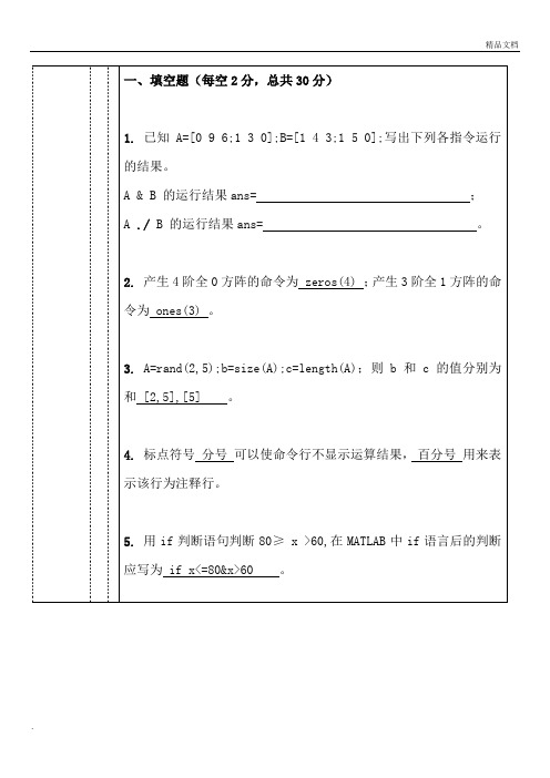
一、填空题(每空2分,总共30分)1.已知A=[0 9 6;1 3 0];B=[1 4 3;1 5 0];写出下列各指令运行的结果。
A &B 的运行结果ans= ;A ./B 的运行结果ans= 。
2. 产生4阶全0方阵的命令为 zeros(4) ;产生3阶全1方阵的命令为 ones(3) 。
3. A=rand(2,5);b=size(A);c=length(A);则b和c的值分别为和 [2,5],[5] 。
4. 标点符号分号可以使命令行不显示运算结果,百分号用来表示该行为注释行。
5. 用if判断语句判断80≥ x >60,在MATLAB中if语言后的判断应写为 if x<=80&x>60 。
6.P, Q分别是个多项式的系数矢量,求P对应的多项式的积分(对应的常数项为K),使用的命令是 polyint(P,K) ;求P/Q的解,商和余数分别保存在k和r,使用的命令是 [k,r]=deconv(P,Q) ;7.为了使两个plot的图形在同一个坐标显示,可以使用 hold on 命令进行图形保持;可以使用 grid on 命令为图形添加网格。
8.MATLAB的工作空间中有三个变量v1, v2, v3,写出把它们保存到文件my_data.mat 中的指令 save my_data ;写出把my_data.mat文件中的变量读取到MATLAB 工作空间内的指令 load my_data 。
二、选择题(每空2分,总共20分)1.下列哪个变量的定义是不合法的 A(A) abcd-3 (B) xyz_3 (C) abcdef (D) x3yz2.下列哪条指令是求矩阵的行列式的值 C(A) inv (B) diag (C) det (D) eig3.在循环结构中跳出循环,执行循环后面代码的命令为 B(A) return (B) break (C) continue (D) keyboard4. 清空Matlab工作空间内所有变量的指令是 C(A) clc (B) cls (C) clear (D) clf5.用round函数四舍五入对数组[2.486.39 3.93 8.52]取整,结果为 C(A) [2 6 3 8] (B) [2 6 4 8] (C) [2 6 4 9] (D) [3 7 4 9]6.已知a=2:2:8, b=2:5,下面的运算表达式中,出错的为 C(A) a'*b (B) a .*b (C) a*b (D) a-b7.角度[]60x,计算其正弦函数的运算为D45=30(A) SIN(deg2rad(x)) (B) SIN(x) (C) sin(x) (D) sin(deg2rad(x))8.下面的程序执行后array的值为 ( A )for k=1:10if k>6break;elsearray(k) = k;endend(A) array = [1, 2, 3, 4, 5, 6] (B) array = [1, 2, 3, 4, 5, 6, 7, 8, 9,10](C) array =6 (D) array =10.9.i=2; a=2i; b=2*i; c=2*sqrt(-1); 程序执行后;a, b, c的值分别是多少?(A)a=4, b=4, c=2.0000i (C)(B)a=4, b=2.0000i, c=2.0000i(C)a=2.0000i, b=4, c=2.0000i(D) a=2.0000i, b=2.0000i, c=2.0000i10. 求解方程x4-4x3+12x-9 = 0 的所有解(A)1.0000, 3.0000, 1.7321, -1.7321(B)1.0000, 3.0000, 1.7321i, -1.7321i(C)1.0000i, 3.0000i, 1.7321, -1.7321(D)-3.0000i, 3.0000i, 1.7321, -1.7321三、写出程序的执行结果或写出给定要求的指令(总共35分)1.写出执行以下代码后C,D,E的值 (6分)A=[1,2,3;4:6;7:9];C=[A;[10,11,12]],D=C(1:3,[2 3])E=C(2,[1 2])2.写出执行以下代码后,MATLAB命令窗口上显示的x矩阵的值 (5分)x=[0,1,0,2,0,3,0,4];for k=1:8if x(k)==0x(k)=k;elsex(k)=2*k+1;endenddisp(x);3.创建符号函数并求解,要求写出步骤和运行结果(7分)(1)创建符号函数f=ax2+bx+c(2)求f=0的解4. 求解以下线性方程组,要求写出程序代码和运行结果(5分)2x1- 3x2+ x3+2x4=8x1+3x2+ x4=6x1- x2+ x3+8x4=17x1+ x2-2x3+2x4=55.绘制函数曲线,要求写出程序代码(12分)(1)在区间[0:2π]均匀的取50个点,构成向量π(2)在同一窗口绘制曲线y1=sin(2*t-0.3); y2=3cos(t+0.5);要求y1曲线为红色点划线,标记点为圆圈;y2为蓝色虚线,标记点为星号四、使用MATLAB语言进行编程(15分)打印出所有的水仙花数。
matlab期末考试题目及答案

matlab期末考试题目及答案1. 题目:编写一个MATLAB函数,实现矩阵的转置操作。
答案:可以使用`transpose`函数或`.'`操作符来实现矩阵的转置。
例如,对于一个矩阵`A`,其转置可以通过`A'`或`transpose(A)`来获得。
2. 题目:使用MATLAB求解线性方程组Ax=b,其中A是一个3x3的矩阵,b是一个3x1的向量。
答案:可以使用MATLAB内置的`\`操作符来求解线性方程组。
例如,如果`A`和`b`已经定义,求解方程组的代码为`x = A\b`。
3. 题目:编写MATLAB代码,计算并绘制函数f(x) = sin(x)在区间[0, 2π]上的图像。
答案:首先定义x的范围,然后计算对应的函数值,并使用`plot`函数绘制图像。
代码示例如下:```matlabx = linspace(0, 2*pi, 100); % 定义x的范围y = sin(x); % 计算函数值plot(x, y); % 绘制图像xlabel('x'); % x轴标签ylabel('sin(x)'); % y轴标签title('Plot of sin(x)'); % 图像标题```4. 题目:使用MATLAB编写一个脚本,实现对一个给定的二维数组进行排序,并输出排序后的结果。
答案:可以使用`sort`函数对数组进行排序。
如果需要对整个数组进行排序,可以使用`sort`函数的两个输出参数来获取排序后的索引和值。
代码示例如下:```matlabA = [3, 1, 4; 1, 5, 9; 2, 6, 5]; % 给定的二维数组[sortedValues, sortedIndices] = sort(A(:)); % 对数组进行排序sortedMatrix = reshape(sortedValues, size(A)); % 将排序后的值重新构造成矩阵disp(sortedMatrix); % 显示排序后的结果```5. 题目:编写MATLAB代码,实现对一个字符串进行加密,加密规则为将每个字符的ASCII码值增加3。
Matlab期末大作业

华南农业大学《控制系统仿真与计算机辅助设计》基于Matlab /Simulink的风力发电机仿真施茂良200830460226陶杰2008304602272012年1月2日题目:用simulink 搭建风力发电机部分的仿真图,使其工作模式满足式(2-4),使用的发电机是永磁同步电机,具体背景材料附后。
风力发电机的控制思路如下:我们需要依据风的速度控制电机的转速使得风能的利用率最高,而电机的转速通过改变永磁同步电机的定子端电压ud 和uq 来实现,具体方程为(3-28)。
最终通过PWM 的导通关断时间来改变端电压,如材料图 2所示。
具体要求:1. 根据公式(2-5)画出类似 图2.3 的曲线。
且当β=0时,画出为获得最大的风能利用率,叶尖速λ和风速v 之间的曲线关系。
风力机用来捕获风能,将叶片迎风扫掠面积内的一部分空气的动能转换为有用的机械能,它决定了整个风力发电系统装置有效功率的输出。
风力机的输入功率是3231122V P A v R v ρρπ==式中,ρ为空气密度;A 为风力机叶片扫掠面积;R 为叶片半径。
v 为风速。
风力机的输出功率为3012p P A v C ρ=式中,pC 为风能利用系数,其值小于1。
风力机输出转矩为;其中λ为叶尖速比 风能利用系数pC 为风力机将风能转换为机械能的效率,它与风速、叶片转速,叶片直径和桨叶节距角均有关系,是叶尖速比λ和桨叶节距角β的函数。
叶尖速比λ是风能叶尖速与风速之比,即R v ωλ=式中,ω为风力机叶片旋转角速度。
根据上文可知,功率与风速具有一定的关系,它们可以用下面的函数来表示213116(,)0.5176(0.45)0.0068110.0350.081i p i iC e λβλβλλλλββ-⎧=--+⎪⎪⎨⎪=-⎪++⎩根据公式(2-5)在simulink 中的建模如图所示:Matlab 波形曲线图其中(β = 0 ,2,5,8,12,15 )代入公式2-5的曲线 蓝色曲线为β=0时风能利用系数p C 与β和λ之间的曲线据根λ=RW/v; 叶尖速λ和转速v 的关系,绘制如下图:2.搭建一个模块,使其产生自然风(5-26),并封装起来,画出一具体的 然风的曲线自然风是非常随机的一种物理现象,其产生机理非常复杂,对其建模也殊为不易。
matlab期末考试题及答案
matlab期末考试题及答案MATLAB期末考试题及答案一、选择题(每题2分,共20分)1. MATLAB中用于创建向量的函数是:A. vectorB. arrayC. linspaceD. ones答案:D2. 下列哪个命令可以计算矩阵的行列式?A. detB. diagC. traceD. rank答案:A3. 在MATLAB中,以下哪个选项是用于绘制三维图形的?A. plotB. plot3C. barD. scatter答案:B4. MATLAB中,用于计算向量范数的函数是:A. normB. meanC. medianD. std答案:A5. 下列哪个命令可以用于创建一个二维数组?A. array2dB. matrixC. create2dD. make2d答案:B6. MATLAB中,用于求解线性方程组的函数是:A. solveB. linsolveC. equationD. linprog答案:A7. 以下哪个函数可以用于生成随机数?A. randB. randomC. randnD. randi答案:A8. MATLAB中,用于实现循环结构的关键字是:A. loopB. forC. whileD. repeat答案:B9. 下列哪个命令可以用于绘制函数图形?A. plotB. graphC. drawD. functionplot答案:A10. MATLAB中,用于计算矩阵特征值的函数是:A. eigB. eigenvalueC. characteristicD. eigen答案:A二、简答题(每题5分,共30分)1. 简述MATLAB中矩阵的基本操作有哪些?答案:矩阵的基本操作包括矩阵的创建、矩阵的加法、减法、乘法、转置、求逆、求行列式等。
2. MATLAB中如何实现条件语句?答案:MATLAB中实现条件语句主要使用if-else结构,也可以使用switch-case结构。
3. 请解释MATLAB中的函数定义方式。
MATLAB期末考试试题(全12套)
MATLAB期末考试试题一、填空(30分)1. 表达式 (3>2)*(5~=5)的类型是(double)。
2. 表达式 (5<2)*120的值是( 0 )。
3. 表达式 (5>2)*(6~=5)的值是( 1 )。
4. 表达式 char(65)=='A' 的值是( 1 )。
5. 表达式 char(65)+1 的值是(66 )。
6. 表达式 'A'+1的值是( 66 )。
7. 表达式 'A'+'B' 的值是(131 )。
8. 存储double型数据占用内存(8 )字节。
9. 存储single型数据占用内存( 4 )字节。
10. 清除命令窗口内容的命令是( clc )。
11. 删除工作空间中保存的变量x的命令是(clearx )。
12. 将双精度实数的显示格式设置成15位定点小数格式的命令是( format long )。
13. 将横坐标轴标签设置成“时间(秒)”的语句是(xlabel('时间(秒)') )。
14. 设置图例的Matlab库函数名是( legend )。
15. 绘制三维线图的Matlab库函数名是( plot3 )。
二、选择题(30分)1. 执行语句x=55后,Matlab将创建变量x,为其分配的存储空间的大小为(C)A)2字节 B)4字节 C)8字节 D)16字节2. 执行语句y=66后,Matlab将创建变量y,其类型为(D )A)int8 B)int16 C)single D)double3. 下列整数类型中,不能参与任何运算的类型为( D )A)int8 B)int16 C)int32 D)int644. 设已执行语句x=3>2; y=x>0后,下面表达式中错误的是( D )A)x+y B)x-y C)x*y D)x/y5. 下列的数组写法中错误的是(C)A)[1:9] B)1:9 C)[1:2:9;2:2:8] D)[1:3;4:6;7:9]6. 设有数组定义:x=[1,2,3,4,5,6], y=x' ,下列表达式中正确的是( D)A)y+x B)y-x C)y./x B)y*x7. 执行语句for x=1:2:10, disp(x), end,循环体将执行几次( B)A)10次 B)5次 C)1次 D)0次8. 函数首部格式为function [out1,out2]=myfunc(in1,in2),不正确的调用格式是(C )A)[x,y]=myfunc() B)myfunc(a,b) C)[x,y]=myfunc(a)D)x=myfunc(a,b)9. 语句 x=-1:0.1:1;plot([x+i*exp(-x.^2);x+i*exp(-2*x.^2);x+i*exp(-4*x.^2)]' ),绘制(B )A)1条曲线 B)3条曲线 C)21条曲线 D)0条曲线10. 下列哪条指令是求矩阵的行列式的值 ( C )A) inv B) diag C) detD) eig三、解答题(40分)1.已知多项式323)(2345+++-=x x x x x f ,1331)(23--+=x x x x g ,写出计算下列问题的MATLAB 命令序列(1))(x f 的根解:>> p1=[3,-1,2,1,3];>> x=roots(p1)x =0.6833 + 0.9251i0.6833 - 0.9251i-0.5166 + 0.6994i-0.5166 - 0.6994i(2))(x g 在闭区间[-1,2]上的最小值解:>> [y,min]=fminbnd(@(x)((1/3)*x.^3+x.^2-3*x-1),-1,2)y =1.0000min =-2.66672.已知 ax -ax e -ex +ay =sin(x +a)+a ln 22, 写出完成下列任务的MATLAB 命令序列。
matlab大作业
大作业
做期末考试的 MATLAB在高等数学课程中的应用(第一、八排同 学) 2. MATLAB在线性代数课程中的应用(第二 排同学) 3. MATLAB在积分变换课程中的应用(第三 排同学) 4. MATLAB在电路课程中的应用(第四 排同学) 5. MATLAB在自控原理课程中的应用(第五、六排同 学) 6. Simulink在自控原理课程中的应用(第 七排同学)
要求
1. 每个人写的都必须不同,否则视为0分。 2. 要求8页左右(打印或手写) 3. 要分成几个小节,每小节按照介绍的功能 划分。 4. 每小节先用文字说明,再使用MATLAB程 序演示,可以使用波形显示结果,前四个 题目MATLAB程序或simulink模型实现。 重要的语句和结果要加文字说明,不重要 的结果不要显示(用;加在语句后面)
MATLAB期末大作业
1.龟兔赛跑本题旨在可视化龟兔赛跑的过程。
比赛的跑道由周长为P面积为A的矩形构成。
每单位时间,乌龟沿跑道缓慢前进一步,而兔子信心满满,每次以一个固定的概率决定走或不走。
如果选择走,就从2-10步中等概率选择一个步长。
每个单位时间用一个循环表示。
赛跑从矩形跑道左上点(0,0)开始,并沿顺时针方向进行。
不管是乌龟或兔子,谁先到达终点,比赛就告结束。
要求:编写MATLAB程序可视化上述过程。
程序以P,A以及兔子每次休息或前进的概率为输入参量。
程序必须可视化每个时刻龟兔赛跑的进程,并以红色“*”表示乌龟,蓝色的“—”表示兔子。
测试时可取P=460,A=9000。
通过上述例子,可否从理论和实验角度估计兔子休息或前进的概率,是的兔子和乌龟在概率意义下打平手。
2.黄金分割Fibonacci数列F n通过如下递推格式定义F n=F n-1+F n-2,其中F0=F1=1要求:1.计算前51项Fibonacci数,并存入一个向量2.利用上述向量计算比值F n/F n-13.验证该比值收敛到黄金比例(1+5)/23.图像处理此题旨在熟悉图像处理的基本操作,请各位自己选择一张彩色图像pMATLAB以三维数组读取一张彩图。
该彩图上每个像素位置分别存放一个取值0-255的三维向量,其三个分量分别表示该点的红(R)绿(G)蓝(B)强度信息。
要求:编写MATLAB程序,读入原始彩色图像,并且在一个图形窗口界面下显示六张图像。
这六张图分别是原始RGB彩图,及其5各变形:RBG,BRG,BGR,GBR和GRB。
每张子图要求以其对应变形命名。
最后将图像以a.jpg形式保存并黏贴至报告中。
提示:imread, imshow, cat。
- 1、下载文档前请自行甄别文档内容的完整性,平台不提供额外的编辑、内容补充、找答案等附加服务。
- 2、"仅部分预览"的文档,不可在线预览部分如存在完整性等问题,可反馈申请退款(可完整预览的文档不适用该条件!)。
- 3、如文档侵犯您的权益,请联系客服反馈,我们会尽快为您处理(人工客服工作时间:9:00-18:30)。
电气学科大类Modern Control SystemsAnalysis and DesignUsing Matlab and Simulink Title: Automobile Velocity ControlName: 巫宇智Student ID: U200811997Class:电气0811电气0811 巫宇智CataloguePreface (3)The Design Introduction (4)Relative Knowledge (5)Design and Analyze (6)Compare and Conclusion (19)After design (20)Appendix (22)Reference (22)Automobile Velocity Control1.Preface:With the high pace of human civilization development, the car has been a common tools for people. However, some problems also arise in such tendency. Among many problems, the velocity control seems to a significant challenge.In a automated highway system, using the velocity control system to maintain the speed of the car can effectively reduce the potential danger of driving a car and also will bring much convenience to drivers.This article aims at the discussion about velocity control system and the compensator to ameliorate the preference of the plant, thus meets the complicated demands from people. The discussion is based on the simulation of MATLAB.Key word: PI controller, root locus电气0811 巫宇智2.The Design Introduction:Figure 2-1 automated highway systemThe figure shows an automated highway system, and according to computing and simulation, a velocity control system for maintaining the velocity if the two automobiles is developed as below.Figure 2-2 velocity control systemThe input, R(s), is the desired relative velocity between the twoAutomobile Velocity Controlvehicles. Our design goal is to develop a controller that can maintain the vehicles in several specification below.DS1 Zero steady-state error to a step inputDS2 Steady-state error due to a ramp input of less than 25% of the input magnitude.DS3 Percent overshoot less than 5% to a step input.DS4 Settling time less than 1.5 seconds to a step input( using a 2% criterion to establish settling time)3.Relative Knowledge:Controller here actually serves as a compensator, and we have some compensators for different specification and system.电气0811 巫宇智4.Design and Analysis:4.1S pecification analysisAccording to the relative knowledge above, I may consider a PI controller to compensate------------G c(s)=k p s+k I.sDs1: zero steady error to step response:To introduce an integral part to add the system type is enough.Ds2: Steady-state error due to a ramp input of less than 25% of the input magnitude.limsGc(s)G(s)≥4 −−→ Ki>4abs→0Ds3: overshoot less than 5% to a step response.P.0≤5% −−→ξ≥0.69DS4 Settling time less than 1.5 seconds to a step input( using a 2% criterion to establish settling time)Ts≤1.5 −−→ξ∗Wn≥2.66According to DS3 and DS4, we can draw the desired regionto placeAutomobile Velocity Controlour close-loop poles.(as the shadow indicate)Figure 4-1 Desired region for locating the dominant polesAfter adding the controller, the system transfer function become:T(s)=Kp s+Kis3+10s2+(16+Kp)s+KiThe corresponding Routh array is:s3 1 Kp+ab s2a+b Kis1ba KiabKpba+-++))((电气0811 巫宇智s0KiFor stability, we have (a+b)(Kp+ab)−Kia+b>0For another consideration, we need to put the break point of root locus to the shadow area in Figure 4-1 to ensure the dominant poles placed on the left of s=-2.66 line.a=−a−b−(−Ki Kp)2<−2.66In all, the specification is equal to a PI controller with limit below.{(a+b)(Kp+ab)−Kia+b>0⋯⋯⋯⋯⋯①KiKp<−5.32+(a+b)⋯⋯⋯⋯⋯⋯⋯②Ki>4ab⋯⋯⋯⋯⋯⋯⋯⋯⋯⋯⋯⋯③4.2Design process:4.2.1Controller verification:At the very beginning, we take the system with G(s)=1(s+2)(s+8)and the controller (provided by the book) withG c(s)=33+66sfor an initial discussion.Automobile Velocity ControlFigure 4-2 step response( a=2,b=8,Kp=33,Ki=66)Figure 4-3 ramp response( a=2,b=8,Kp=33,Ki=66)电气0811 巫宇智From figure 4-2, we can see that the overshoot is 4.75%, and the settling time is 1.04 s with zero error to the step input.From figure 4-3, it is clear that the ramp steady-state error is a little less than 25%.Thus, the controller with G c(s)=33+66scompletely meets the specification .4.2.2further analysis:For next procedure, I will have some more specific discussion about the applicable range of this controller to see how much can a and b vary yet allow the system to remain stable.We don’t change the parameter of the controller, and insert the Ki=66, Kp=33 into the inequality and get this:.{ab<16.5a+b>7.32ab+33−66a+b>0If we suppose the system to be a minimum phase system, a,b>0,thus it is easy to verify the 3rd inequality. Now, we draw to see the range of a and b.Figure4-4 the range of a,b for controller(Kp=33,Ki=66)Actually, the shade area can not completely meets the specification, for the constraint conditions represented in the 3 inequality is not enough, we need to draw the root locus for a certain system(a and b) to locate the actual limit for controller.However, this task is rather difficult, in a way, the 4 variables (a,b,Ki,Kp) all vary in terms of others’ change . Thus we can approximately locate the range of a and b from the figure above.4.2.3Alternatives discussion:According to inequality ①②③,The range of a and b bear some relation with the inequality below:{ a +b >5.32+Ki Kp ab <Ki 4Kp +ab −Ki a +b >0Basing our assumption on the range in the previous discussion, we can easily see that in order to increase the range, we can increase Ki and decrease the ratio of Ki to Kp.Thus, I adjust the parameter to{Ki =80Kp =64Figure4-5 the range of a,b for controller(Kp=64,Ki=80)As the figure indicate,(the range between dotted lines refers tothe previous controller, while the range between red lines refers to the new alternatives), the range increase as we expect.Next step, we may keep the system of G(s)=1(s+2)(s+8)fixed, and discuss the different compensating effect of different PI parameter.When carefully checking the controller, we may find that the controller actually add a zero( -Ki/Kp) , an integral part and a gain part, so we can only change the zero and draw the locus root and examine the step response and ramp response.KiKp=1.5:Figure4-6 the root locus (KiKp=1.5)Using rlocfind, we find the maximum Kp=34.8740So we choose 3 groups of parameter ([35,52.5],[30.45],[25,37.5]) to examine the reponseFigure4-7 the step response (KiKp=1.5)It’s clear that the step response preference is not satisfying with too long settling timeKiKp=2:Figure4-8 the root locus (KiKp=2)Using rlocfind, we find the maximum Kp=34.3673So we choose 3 groups of parameter to examine the response and ramp response.Figure4-9 the step response (KiKp=2)Figure4-10 the ramp response (KiKp=2)KiKp=2.5:Figure4-11 the root locus (KiKp=2.5)Using rlocfind, we find the maximum Kp=31.47Similarly, we choose 3 groups of parameter to examine the response and ramp response.Figure4-12 the step response (KiKp=2.5)Virtually, the overshoot (Kp=30, Ki=75) doesn’t meet thespecification as we expect. I guess, that may come from the effect ofzero(-2.5), thus , go back to the step response of KiKp=2, due to the elimination between zero(-2) and poles, thus the preference is within our expectation.Figure4-13 the ramp response (KiKp=2.5)pare and ConclusionMainly from the step response and ramp response, it can be concluded that, in a certain ratio of Ki to Kp, the larger Kp brings smaller ramp response error, as well as larger range of applicable system. Nevertheless, the larger Kp means worse step response preference(including overshoot and settling time).This contradiction is rather common in control system.In all, to get the most satisfying preference, we need to balanceall the parameter to make a compromise, but not a single parameter.From what we are talking about, we find the controller provided by the book(Kp=33, Ki=66) may be one of the best controller in comparison to some degree, with satisfying step response and ramp response preference, as well as a wider range for the variation of a and b, further, it use a zero(s=-2) to transfer the 3rd order system to 2nd order system, in doing so, we may eliminate some unexpected influence from the zero.The controller verified above (in Figure4-9 and Figure 4-10) with Kp=34, Kp=68 may be a little better, but only a little, and it doesn’t leave some margin.6.After Design这是一次艰难,且漫长的大作业,连续一个星期,每天忙到晚上3点,总算完成了这个设计,至少我自己是很满意的。