离散方式对比例谐振控制器PR的影响
比例谐振控制算法分析
身与H z 的关系,因此,在使用脉冲响应不变法时,从H s 到H z 并没有一个由 S 平面到 Z 平面的简单代数映射关系,即没有一个s f z 的代数关系式。
另外, 数字滤波器的频响也不是简单地重现模拟滤波器的频响应, 而是模拟滤波器频响 的周期延拓,周期为Ω H e ∑ 2πf 。即 H jΩ j ∑ H j
KR
= =
A
KR
B
,
其中A
K R ωC 1
C
; B
K R ωC 1
C
将上式通过脉冲响应不变法转成 z 变换,得:
G z Z = e
AZ
T A
T
BZ Z e
B
T
T
,
设 C= e
T
;D= e
T
,则:
G z =
A C
B D
A B C D
AD BC CD
设 Y=GX,则转成差分函数后,该式可表达成: y n 其中:A C D y n 1
KR
控制器波特图如下图所示,从图中所示,控制器在基波频率处的幅频特性为
A ω
60dB.同时相角裕度为无穷大,因此基本可以实现零稳态误差,同时具有很好的稳
态裕度和暂态性能。
3 准 PR 控制器的参数设置
由此可见,除了比例系数外,准 PR 控制器主要有K R 、ω 两个参数。为了分析每个参 数对控制器的影响, 可先假设其余参数不变, 然后观察这个参数变化时间对系统性能的影响。
KR
φ ,该环节的时域响应分析如下:
φ
= L M sin ωt cosφ
Mcos ωt sinφ)= Mcosφ
Msinφ
后的表达式为: Msinφ cosφ
单级式光伏并网逆变器的PR和MPPT集成控制策略

单级式光伏并网逆变器的PR和MPPT集成控制策略闫彩霞;王生铁;张计科【摘要】单级式光伏并网逆变器具有结构简单,成本低、效率高的优点,尤其适合于大容量光伏并网发电系统.针对单级式光伏并网逆变器,提出了一种结合PR和MPPT控制的集成控制策略,它具有功率外环和电流内环的结构,可以同时实现最大功率无差跟踪控制和单位功率因数并网控制.建立了α-β坐标系下的逆变器系统数学模型,给出了结合根轨迹和频率特性的PR控制器参数设计方法,并进行了参数设计.建立了10 kW单级式光伏并网发电系统的仿真模型,仿真结果表明,在模拟标准光强、云朵飘过及全天光照的条件下,PR和MPPT集成控制策略能够快速跟踪光照的变化,实现MPPT的无差跟踪控制及单位功率因数并网控制,具有良好的动静态性能.【期刊名称】《电气传动》【年(卷),期】2014(044)005【总页数】6页(P7-12)【关键词】光伏发电;单级式并网逆变器;比例谐振控制;最大功率跟踪控制;集成控制策略【作者】闫彩霞;王生铁;张计科【作者单位】内蒙古工业大学电力学院,内蒙古呼和浩特010080;内蒙古工业大学电力学院,内蒙古呼和浩特010080;内蒙古工业大学电力学院,内蒙古呼和浩特010080【正文语种】中文【中图分类】TM615;TM464按光伏并网逆变器的结构划分,并网系统主要有单级式和两级式两种拓扑结构[1-2]。
对于大容量光伏并网逆变器,与两级式相比,单级式具有结构简单、成本低、效率高的优点[3-5]。
单级式光伏并网系统主电路拓扑结构如图1所示。
对于单级式光伏并网逆变器的控制,三相系统一般采用在两相旋转坐标系下基于PI控制器的电网电压定向矢量控制,MPPT环节采用电压寻优方式,外环将检测到的直流母线电压与MPPT输出电压值做差,送入PI控制器,输出电流指令;内环主要是控制并网电流,使其跟踪电压外环输出的指令电流。
这种控制是功率、电压、电流3环控制结构,两相旋转坐标系下的控制需要经过多次坐标变换,并且需要前馈解耦控制,结构较复杂[6-7]。
基于PR控制器的永磁同步电机弱磁控制研究
基于PR控制器的永磁同步电机弱磁控制研究肖文英;黄守道【摘要】讲述了永磁同步电机( PMSM)的运行原理,根据其数学模型对其弱磁原理进行介绍.传统的永磁同步电机控制通常使用PI调节器的方法,通过一系列坐标变换将交流量转为直流值,并用PI调节器对其进行跟踪,为达到良好效果,常需附加随系统运行温度变换的交叉耦合项和前馈补偿项,使整个控制系统的鲁棒性降低,在额定转速以上比较高的速度运行时其负面影响尤为明显.分析了比例谐振(proportional resonant,PR)控制器特,提出了一种基于PR控制器及转子磁链定向的移相弱磁控制策略.最后用MATLAB进行仿真,结果表明该控制策略具有良好的鲁棒性和动态性能,验证了该方法的正确性.%This paper described the operating principles of permanent magnet synchronous motor, and introduced weakening principle due to its mathematical models. In the traditional control method of permanent magnet synchronous motor, it usually uses PI adjuster, through a series of coordinate transformation exchanging AC signal to dc signal, and does the tracking by PI adjuster, to achieve good results. It often needs additional cross coupling term and a feed-forward compensation changed with system operation temperature, making the robustness of the whole control system reduced. When speed is high above the rated one, its negative influence is especially remarkable. The paper analyzed the proportional resonant (PR) controller features, combined with permanent magnet synchronous motor mathematical model, and presented a control method based on a PR controller and phase-shift flux weakening control strategy. Finally, MATLAB was used tosimulate die model above. Results show the system got good dynamic and static responses, verifying the correctness and feasibility of the proposed method.【期刊名称】《湘潭大学自然科学学报》【年(卷),期】2011(033)004【总页数】5页(P108-112)【关键词】永磁同步电机;PR控制器;转子磁链定向矢量控制【作者】肖文英;黄守道【作者单位】湖南工学院电气与信息工程系,湖南衡阳421002;湖南大学电气与信息工程学院,湖南长沙410082【正文语种】中文【中图分类】TM571近年来,因变频调速的永磁同步电动机(简称PMSM)具有可靠性高、功率因数和效率高等诸多优点获得了广泛研究和应用[1,2],但其转子励磁固定,运行时要求端电压和速度成正比,因而无法运行到较高的转速和在高速下做恒功率运行.针对此问题采用弱磁控制以获得宽广的调速范围,实现高速恒功率运行.永磁同步电动机弱磁控制有多种方案,其中一种为移相弱磁控制方案[3],其思路类似于开关磁阻电机高速运行模式下的超前移相控制,不需要增加过多的驱动器硬件成本,有着广泛的应用前景.PI控制具有算法简单和可靠性高的特点.因此传统PMSM控制系统常采用PI控制器[4,5].因其只能对直流量有良好的跟踪效果,故坐标变换会增多,会使控制算法难于实现,而PI调节器只能对直流量进行跟踪控制,对交流量无法跟踪[6,7].而且,为达到良好效果,常附加了随系统运行温度变换的交叉耦合项和前馈补偿项,使整个控制系统的鲁棒性降低,特别是在额定转速以上的弱磁运行时,因参数的变化,其影响更大.针对此问题,需寻找到其他方法以克服其缺点.研究发现PR 控制器可以直接对交流量实现无差跟踪,省去了过多的坐标变化,使控制算法更为简单,不用考虑交叉耦合项以及前馈补偿项,优化了系统鲁棒性能[8].因此,本文设计了一种基于PR的控制器的控制方法,并将之应用于永磁同步电机系统控制系统中,采用移相弱磁控制策略,减小了控制算法实现难度,提高了控制系统的鲁棒性和稳定性,同时能实现高转速弱磁的稳定控制.1 永磁同步电动机的矢量控制基于永磁同步电机控制原理,不计电动机的铁心饱和、涡流和磁滞损耗、略磁场中所有的空间谐波、参数变化等因素,旋转坐标系d,q轴下PMSM定子磁链方程为:其中:Ld、Lq为PMSM的d,q轴电感;Id、Iq为定子电流矢量的d,q轴电流;ψr 为转子磁链在定子上的耦合磁链.PMSM在d,q轴上的定子电压方程式:其中:Vd是定子电压矢量V的d轴分量;Vq是定子电压矢量V的q轴分量;p是微分算子;ωr是转子旋转角速度.当d轴与转子主磁通方向一致时,且认为旋转坐标系的旋转角频率与转子旋转角频率一致,可得到PMSM转子磁通定向的电压回路方程式为:电磁转矩方程为:其中:P为电机的极对数.基速以下采用转子磁链定向的PMSM定子电流矢量位于q 轴,无d轴分量,即Iq=I,Id=0,则PMSM的电压方程可写为:电磁转矩方程可简化为:由(6)可知,基速以下,控制Iq就能控制转速实现矢量控制.2 永磁同步电动机的弱磁控制原理永磁同步电机的电压方程可写为:从式(7)可以看到,永磁同步电机的转速和电机端电压成正比,因此当电机达到额定转速后,若要维持电机端电压不变而进一步提高转速,只有靠调节id、iq来实现,即弱磁控制,其一般是通过增加直轴去磁电流分量.永磁同步电机的弱磁扩速控制可由如图1所示的定子电流矢量轨迹加以说明.首先,电机恒转矩运行,即沿着最大转矩比电流曲线OA运行.当电机的电压和电流均达到极限值时,此时转速ω1为对应最大转矩TA时电机的转折速度.若要进一步提高转速,比如将其升至ω2,同时最大限度的利用逆变器容量,则需要控制电流矢量沿着电流极限圆,即AB段逆时针向下运行.从图上可以看出,电流矢量从A点运行到B点,直轴去磁电流分量增大了,同时,电机的输出转矩变小了,即恒功率运行.传统的弱磁方式之一为移相角弱磁控制,如图2所示,当电流矢量为is1时,若此时电机对应最大转矩时的转折速度ω1,为了实现弱磁,即增加直轴去磁电流分量,可将is1对应的角度θ1增大到θ2.由图2可知,此时直轴电流去磁分量增大了.为了实现移相弱磁控制,我们需要求出弱磁调节系数,该系数由下式给定:3 基于PR的PMSM弱磁控制策略PR(proportional resonant)控制器,它的传递函数可如下表示其中,Ki是积分时间常数;Kp为比例常数;w0是谐振频率,而且有作其波特图如图3所示.由图3可以看到,在频率点w0处为高增益,因此可以应用于无静差的电流跟踪控制系统中.其原理框图如图4所示.图5 移相弱磁控制系统框图Fig.5 Phase shifting flux weakening control system在上述基础上,在控制系统中引入PR控制器,将能优化系统的响应.基于PR控制器的移相弱磁控制系统框图如图5所示.图5中,实测的调节系数M与设定值M*做差比较后,其差值通过弱磁环的调节输出角度的给定值.当差值大于0时,弱磁环输出的角度值不发生变换;而当差值小于0时,弱磁环输出的角度值增大,即进入弱磁控制,完成了系统从电流id=0控制过渡到弱磁控制,从恒转矩控制过度到恒功率控制.易知,该控制下,省略了受温度影响的电路参数交叉解耦项ωLiq、ωLid和前馈补偿项ωΨr,从而实现了鲁棒性能高的目的.4 仿真结果及其分析利用MATLAB仿真工具箱,对引入PR控制器的PMSM采用移相弱磁方法,研究其系统控制.永磁电机的参数如表1所示.给定转速设置为:初始值n*=2 000r/min,t=0.15 s时突变,为n*=4 000 r/min.且在t=0.72 s时,突加TL=5 N·m.表1 PMSM参数Tab.1 The PMSM parameter定子额定电压/V定子电阻/Ω转子磁链/Wb定子电感Ld/mH电机极对数定子电感Lq /mH 1000.031 860.055 61.2961.29从图6可以看到,转速给定由2 000 r/min突变为4 000 r/min的过程中,实际转速能平滑地过渡,并进入弱磁扩速状态,系统很好地实现了2倍扩速,且在t=0.72 s负载突变时几乎无脉动,这说明了采用PR控制器能获得良好的动静态转速响应.从图7可以看到,t=0.15 s移相弱磁角由开始为0慢慢向负方向增加,这说明了电机此时在移相弱磁控制下开始进入弱磁运行方式.图8描述了在电机启动时、给定的转速突变情况下以及负载突变的条件下电机的电磁转矩的响应情况.可以看到电磁转矩波动非常小,表明了应用上述控制策略情况下控制系统具有良好的动态性能.图9和图10分别为电机定子三相电流及其细节图的波形,在弱磁扩速达到给定值时突加负载瞬间三相电流有些脉动,但很快达到稳定状态,从图10可见其正弦性能良好.图11和图12分别是定子给定电流和实际电流在静止坐标系下的α分量及其细节图.可以看到,其波形几乎重合,可以说明,在PR控制器对正弦电流的跟踪效果非常好,几乎没有什么偏差,可见其实际应用优势.5 结论PR控制器能够对交流量进行无差跟踪,本文据此进行数学建模,并结合永磁同步转子磁链定向原理,采用移相弱磁方法,建立了PMSM弱磁控制系统仿真模型,并分析了仿真结果.系统的静态性能和动态性能均表现良好,验证了该方法的可行性.参考文献[1]曹荣昌.永磁同步电机牵入同步分析[J].湘潭大学自然科学学报,1999(03):97—99.[2]王旭红,汪建平.永磁同步电动机的研制及优化[J].湘潭大学自然科学学报,2002,24(3):96—99.[3]童怀,刘继辉.永磁同步电动机移相弱磁控制的仿真分析[J].微特电机,2006(8):17—20[4]戴朝波,林海雪.电压源型逆变器三角载波电流控制新方法[J].中国电机工程学报,2002,22(2):99—102.[5]姜俊峰,刘会金,陈允平,等.有源滤波器的电压空间矢量双滞环电流控制新方法[J].中国电机工程学报,2004,24(10):82—86.[6]唐欣,罗安,涂春鸣.基于递推积分PI的混合型有源电力滤波器电流控制[J].中国电机工程学报,2003,23(10):38—41.[7]孙强,程明,周鹗,等.新型双凸极永磁电机调速系统的变参数PI控制[J].中国电机工程学报,2003,23(6):117—122.[8] TEODORESCU R,BLAABJERG F,BORUP U,et al.A new control structure for grid-connected LCL PV inverters with zero steady-state error and selective harmonic compensation[J].IEEE Trans on Power Electronics,2004:580—586.。
PR调节器在电子负载逆变侧控制中的应用
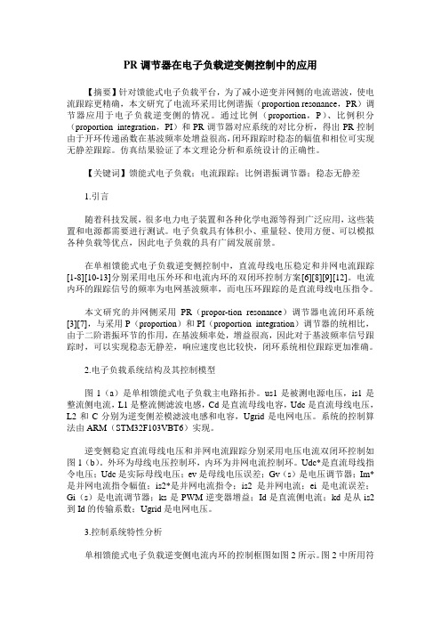
PR调节器在电子负载逆变侧控制中的应用【摘要】针对馈能式电子负载平台,为了减小逆变并网侧的电流谐波,使电流跟踪更精确,本文研究了电流环采用比例谐振(proportion resonance,PR)调节器应用于电子负载逆变侧的情况。
通过比例(proportion,P)、比例积分(proportion integration,PI)和PR调节器对应系统的对比分析,得出PR控制由于开环传递函数在基波频率处增益很高,闭环跟踪时稳态的幅值和相位可实现无静差跟踪。
仿真结果验证了本文理论分析和系统设计的正确性。
【关键词】馈能式电子负载;电流跟踪;比例谐振调节器;稳态无静差1.引言随着科技发展,很多电力电子装置和各种化学电源等得到广泛应用,这些装置和电源都需要进行测试。
电子负载具有体积小、重量轻、使用方便、可以模拟各种负载等优点,因此电子负载的具有广阔发展前景。
在单相馈能式电子负载逆变侧控制中,直流母线电压稳定和并网电流跟踪[1-8][10-13]分别采用电压外环和电流内环的双闭环控制方案[6][8][9][12]。
电流内环的跟踪信号的频率为电网基波频率,而电压环跟踪的是直流母线电压指令。
本文研究的并网侧采用PR(propor-tion resonance)调节器电流闭环系统[3][7],与采用P(proportion)和PI(proportion integration)调节器的统相比,由于二阶谐振环节的作用,在基波频率处,增益很高,因此对于基波频率信号跟踪时,可以实现稳态无静差,响应速度也比较快,闭环系统相位跟踪更加准确。
2.电子负载系统结构及其控制模型图1(a)是单相馈能式电子负载主电路拓扑。
us1是被测电源电压,is1是整流侧电流,L1是整流侧滤波电感,Cd是直流母线电容,Udc是直流母线电压,L2和C分别为逆变侧差模滤波电感和电容,Ugrid是电网电压。
系统的控制算法由ARM(STM32F103VBT6)实现。
离散控制系统的性能指标评估与优化

离散控制系统的性能指标评估与优化离散控制系统是指由离散信号进行控制的系统,它在工业自动化领域中起着重要的作用。
离散控制系统的性能指标评估与优化是改进系统响应、提高控制效果的关键环节。
本文将从离散控制系统的性能指标评估、常见优化方法以及实例分析三个方面进行论述。
一、离散控制系统的性能指标评估离散控制系统的性能评估是对系统的控制效果进行客观、定量的衡量。
常见的性能指标包括稳态误差、动态响应特性和稳定性等。
1. 稳态误差稳态误差是系统输出与期望输出之间的差异,反映了系统的稳态控制精度。
常见的稳态误差指标包括零误差常数Kp、静态误差和稳定误差。
2. 动态响应特性动态响应特性是指系统对输入信号的响应速度和质量。
常用的动态响应特性指标有上升时间Tr、峰值时间Tp、超调量Mp和调节时间Ts。
3. 稳定性稳定性是保证系统正常工作的基本要求,用于评估系统是否具有良好的鲁棒性和稳定性。
常见的稳定性指标包括极点位置、幅值裕度和相位裕度等。
二、离散控制系统的优化方法离散控制系统的优化方法旨在改善系统的性能指标,提高系统的控制效果。
常见的优化方法包括PID控制器参数调整、模型预测控制、最优控制和自适应控制等。
1. PID控制器参数调整PID控制器是离散控制系统中常用的控制器,通过合理地调整PID控制器的参数可以改善系统的稳态误差和动态响应特性。
常用的参数调整方法有经验法则法、Ziegler-Nichols法和模糊PID控制等。
2. 模型预测控制模型预测控制是一种基于系统模型进行预测的控制方法,通过优化控制输入来实现系统的性能优化。
它可以对系统的未来状态进行预测,并在当前时刻采取合适的控制动作。
常用的模型预测控制方法有基于模型的预测控制和自适应模型预测控制等。
3. 最优控制最优控制方法通过优化控制输入来实现系统性能的最优化。
常用的最优控制方法包括线性二次调节器(LQR)、最优随机控制和最优动态规划等。
4. 自适应控制自适应控制方法是指根据系统的实时情况自动调整控制参数以适应系统的变化。
基于PR调节器的并网型逆变器谐波抑制策略

基于PR调节器的并网型逆变器谐波抑制策略王印松;王姝媛;海日【摘要】解决LCL型并网逆变器谐振问题的有效途径是采用电容电流反馈的有源阻尼法,比例谐振(PR)调节器因具有良好的准确性和抗干扰性能,比PI调节器更适于对并网电流控制,但电网电压背景谐波会使并网电能质量变差.提出了一种基于电网电压微分前馈和PR调节器相结合的双闭环控制策略,经过适当变换,电容电流内环等效为网侧电感电压微分反馈,电网电压前馈等效为比例前馈.仿真实验结果表明,基于电网电压微分前馈和PR调节器相结合的控制策略可以基本避免电网电压谐波影响并网电能质量,且该策略可以省去对三相电容电流的检测,在很大程度上节约了成本.【期刊名称】《电源技术》【年(卷),期】2016(040)001【总页数】5页(P184-188)【关键词】LCL滤波器;并网逆变器;PR调节器;并网电流;背景谐波【作者】王印松;王姝媛;海日【作者单位】华北电力大学控制与计算机工程学院,河北保定071003;中国电力科学研究院计量研究所,北京100192;华北电力大学控制与计算机工程学院,河北保定071003【正文语种】中文【中图分类】TM464在追求低碳社会的今天,可再生能源如太阳能,因其储量丰富、无污染逐渐得到了世界各国的广泛关注。
太阳能利用的主要方式是太阳能光伏并网发电。
光伏并网逆变器是光伏系统能量转换与控制的核心,其作用是把光伏电池阵列输出的直流电能转换成能并入电网的交流电能。
L型滤波和LCL型滤波在光伏并网逆变器输出滤波器中应用较多[1]。
相比于L滤波器,LCL型滤波器具有三阶的低通滤波特性,因而对于同样谐波标准和较低的开关频率,可以采用相对较小的滤波电感设计,有效减小系统体积并降低损耗[2]。
通常用PI或PR调节器来进行光伏系统并网控制。
PI调本文针对文献[6]中存在的问题进行了一定的改进,提出一种基于电网电压微分前馈和PR调节器相结合的并网电流双闭环控制策略,等效变换为基于电网电压比例前馈的网侧电感电压微分反馈内环,并网电流外环策略,通过Matlab/Simulink仿真实验验证了本文所提控制策略的正确性。
基于改进PR控制的多功能逆变器控制策略

基于改进PR控制的多功能逆变器控制策略刘亚峰;陈羽;彭克;刘国栋【摘要】多功能并网逆变器(multi-functional grid-tied inverter,MFGTI)在实现分布式电源(Distributed Generation,DG)并网的同时能够兼具电能质量治理的功能,相比功能单一的并网逆变器,具有更好的应用前景.针对分布式电源的多功能并网逆变器进行研究,针对传统PR控制器,提出一种基于改进PR控制的多功能逆变器跟踪控制方法,除了并网控制外还兼具了滤除谐波电流的功能.设计了应用多层PIR 控制器的双环PQ逆变器控制,使并网的分布式电源除了提供功率以外还能够有效滤除特定次数谐波.建立该控制系统的数学模型并且利用DIGSILENT/PowerFactory对其进行仿真,验证了该控制系统的正确性和有效性.仿真结果表明,所提出的多功能逆变器除了能够改善并网点的电能质量,还能够满足微网的要求,对并网点进行PQ控制.【期刊名称】《山东电力技术》【年(卷),期】2017(044)006【总页数】6页(P35-40)【关键词】分布式发电;谐波补偿;多功能逆变器;PIR控制【作者】刘亚峰;陈羽;彭克;刘国栋【作者单位】山东理工大学电气与电子工程学院,山东淄博 255049;山东理工大学电气与电子工程学院,山东淄博 255049;山东理工大学电气与电子工程学院,山东淄博 255049;山东理工大学电气与电子工程学院,山东淄博 255049【正文语种】中文【中图分类】TM72分布式发电系统是应对环境污染、应用清洁能源的有效途径,也是解决能源危机、利用可持续能源的较为现实的方式,近年来分布式电源(DG)得到了越来越多的重视[1]。
如何将不可控的分布式电源以更高的电能质量稳定地接入电网便成了研究的热点。
分布式电源一般通过并网逆变器接入微电网中。
已经有学者对并网逆变器的拓扑以及控制策略进行了大量的研究[2-5]。
单相PWM整流器比例谐振控制与前馈补偿控制

单相PWM整流器比例谐振控制与前馈补偿控制李立;赵葵银;徐昕远;朱建林【摘要】提出了单相PWM整流器比例-谐振控制(PR)与无延迟前馈补偿控制的策略.系统由比例-谐振控制器、快速的相角估计器和无延迟前馈补偿器组成.与传统的PI控制器和多频率比例-谐振电流控制器相比,该比例谐振控制器结构简单,能显著减少控制延迟时间.通过理论分析,提出的用电网电压和电流的估计值与单步预测值来实现的无延迟前馈补偿器,可避免因延时引起的不良影响、测量噪音及补偿过程中产生的电网电压谐波分量.仿真分析与实验结果验证了系统具有较好的稳态性能和更好的抗扰性能.【期刊名称】《电力系统保护与控制》【年(卷),期】2010(038)009【总页数】6页(P75-79,95)【关键词】PWM整流器;比例-谐振控制;前馈补偿器;相角估计器;延迟时间【作者】李立;赵葵银;徐昕远;朱建林【作者单位】湖南工程学院电气信息学院,湖南,湘潭,411101;湖南工程学院电气信息学院,湖南,湘潭,411101;湖南省电力公司长沙电业局,湖南,长沙,410015;湘潭大学,湖南,湘潭,411105【正文语种】中文【中图分类】TM770 引言PWM 整流器具有输入电压电流同相位、可实现单位功率因数、可四象限运行等诸多优点,因而具有广泛的应用前景[1-3]。
目前常用的电流控制方法有PI、滞环控制。
PI控制具有算法简单和可靠性高的特点,且常规的PI控制只能消除直流参考信号的稳态误差,对给定值中的交流分量难以进行无差跟踪[4-8]。
滞环控制具有电路简单、动态响应快的特点,但是开关频率、损耗及控制精度受滞环宽度的影响[4]。
对交流信号而言,比例谐振控制在基波频率处增益无穷大,可以实现系统零稳态误差[7,9]。
本文利用比例谐振控制算法能够在静止坐标系下对交流信号进行无静差调节的优势[10],并考虑比例-谐振(Proportional-resonant -PR)控制算法虽然控制精度很高,但实时性却不够[11],提出一种新的单相PWM整流器的PR控制策略。
- 1、下载文档前请自行甄别文档内容的完整性,平台不提供额外的编辑、内容补充、找答案等附加服务。
- 2、"仅部分预览"的文档,不可在线预览部分如存在完整性等问题,可反馈申请退款(可完整预览的文档不适用该条件!)。
- 3、如文档侵犯您的权益,请联系客服反馈,我们会尽快为您处理(人工客服工作时间:9:00-18:30)。
Effects of Discretization Methods on the Performance of Resonant ControllersAlejandro G.Yepes,Student Member,IEEE,Francisco D.Freijedo,Member,IEEE, Jes´u s Doval-Gandoy,Member,IEEE,´Oscar L´o pez,Member,IEEE,Jano Malvar,Student Member,IEEE,and Pablo Fernandez-Comesa˜n a,Student Member,IEEEAbstract—Resonant controllers have gained significant impor-tance in recent years in multiple applications.Because of their high selectivity,their performance is very dependent on the ac-curacy of the resonant frequency.An exhaustive study about dif-ferent discrete-time implementations is contributed in this paper. Some methods,such as the popular ones based on two integrators, cause that the resonant peaks differ from expected.Such inac-curacies result in significant loss of performance,especially for tracking high-frequency signals,since infinite gain at the expected frequency is not achieved,and therefore,zero steady-state error is not assured.Other discretization techniques are demonstrated to be more reliable.The effect on zeros is also analyzed,establishing the influence of each method on the stability.Finally,the study is extended to the discretization of the schemes with delay compensa-tion,which is also proved to be of great importance in relation with their performance.A single-phase active powerfilter laboratory prototype has been implemented and tested.Experimental results provide a real-time comparison among discretization strategies, which validate the theoretical analysis.The optimum discrete-time implementation alternatives are assessed and summarized.Index Terms—Current control,digital control,power condition-ing,pulsewidth-modulated power converters,Z transforms.N OMENCLATUREVariablesC Capacitance.f Frequency in hertz.G(s)Model in the s domain.G(z)Model in the z domain.H(s)Resonant controller in the s domain.H(z)Resonant controller in the z domain.i Current.K Gain of resonant controller.L Inductance value.m Pulsewidth modulation(PWM)duty cycle. N Number of samples to compensate with com-putational delay compensation.n Highest harmonic to be compensated. Manuscript received September17,2009;revised December29,2009.Date of current version June18,2010.This work was supported by the Spanish Min-istry of Education and Science under Project DPI2009-07004.Recommended for publication by Associate Editor P.Mattavelli.The authors are with the Department of Electronic Technology,University of Vigo,Vigo36200,Spain(e-mail:agyepes@uvigo.es;fdfrei@uvigo.es;jdoval@ uvigo.es;olopez@uvigo.es;janomalvar@uvigo.es;pablofercom@uvigo.es). Color versions of one or more of thefigures in this paper are available online at .Digital Object Identifier10.1109/TPEL.2010.2041256R Equivalent series resistance value.R(s)Resonant term in the s domain.R(z)Resonant term in the z domain.T Period.θPhase of grid voltage.V V oltage.ωAngular frequency in radians per second.u(s)Input value.y(s)Output value.Subscripts1Fundamental component.a Actual value(f).c Generic current controller(G).d Degree of freedom in the zero-pole matchingdiscretization method(K).dc Relative to the dc link(V).f Relative to the passive inductivefilter(V,i,L,R,and G).I Equivalent to the double of the integral gainof a proportional+integral(PI)controller indq frame(K).k Relative to the k th harmonic(H,R,K P,andK I).L Relative to the load(i).Lh Relative to the harmonics of the load(i).o Resonant frequency of a continuous resonantterm or resonant controller(f andω).P Equivalent to the double of the proportionalgain of a PI controller in dq frame(K). PCC Relative to the point of common coupling(V).PL Relative to the plant(G).rms Root mean square.s Relative to sampling(f and T).src Relative to the voltage source(V,i,and L). sw Relative to switching(f).T Sum of the gains for every value of harmonicorder k(K P).X Resonant term R or resonant controller Hdiscretized with method X,where X∈{zoh,foh,f,b,t,tp,zpm,imp}.X&Y Resonant term R or resonant controller Himplemented with two discrete integrators,with the direct one discretized with method Xand the feedback one with method Y,whereX,Y∈{zoh,foh,f,b,t,tp,zpm,imp}.0885-8993/$26.00©2010IEEEX−Y Resonant controller H VPI(z),in whichR1(s)is discretized with method X andR2(s)with method Y,where X,Y∈{zoh,foh,f,b,t,tp,zpm,imp}. Superscripts∗Reference value.1Resonant term R of the form s/(s2+ω2o). 2Resonant term R of the form s2/(s2+ω2o).d Including delay compensation(H and R). PR Resonant controller H of the PR type.VPI Resonant controller H of the VPI type. Others∆x Difference between x and its target value(i f).ˆx Estimated value of x(θ1andω1).I.I NTRODUCTIONI N recent years,resonant controllers have gained significantimportance in a wide range of different applications due to their overall good performance.They have been applied with satisfactory results to cases such as distributed power generation systems[1],[2],dynamic voltage regulators[3],[4],wind tur-bines[5],[6],photovoltaic systems[7],[8],fuel cells[9],[10], active rectifiers[11],active powerfilters(APFs)[12]–[17], microgrids[18],and permanent magnet synchronous motors [19].Resonant controllers allow to track sinusoidal references of arbitrary frequencies with zero steady-state error for both single-phase and three-phase applications.An important saving of computational burden and complexity is obtained due to their implementation in stationary frame,avoiding the coordinates transformations,and providing perfect tracking of both positive and negative sequences[1],[13],[14],[20]–[22].Resonant con-trollers in synchronous reference frame(SRF)have been also proposed to control pairs of harmonics simultaneously when no unbalance exist[7],[15]–[17],[22],[23].An essential step in the implementation of resonant digital controllers is the discretization.Because of the narrow band and infinite gain of resonant controllers,they are specially sensitive to this process.Actually,a slight displacement of the resonant poles causes a significant loss of performance.In the case of proportional+resonant(PR)controllers[14],[20]–[22],even for small frequency deviations,the effect of resonant terms becomes minimal,and the PR controller behaves just as a proportional one[14].The resonant regulator proposed in[16]is less sensitive to these variations when cross coupling due to the plant appears in the dq frame,but if these deviations in the resonant poles are present,it does not achieve zero steady-state error either. Furthermore,if selectivity is reduced to increase robustness to frequency variations,undesired frequencies and noise may be amplified.Thus,an accurate peak position is preferable to low selectivity.Therefore,it is of paramount importance to study the effectiveness of the different alternatives of discretization for implementing digital resonant controllers,due to the critical characteristics of their frequency response.As proved in this paper,many of the existing discretization techniques cause a displacement of the poles.This fact results in a deviation of the frequency at which the infinite gain occurs with respect to the expected resonant frequency.This error becomes more significant as the sampling time and the desired peak frequency increase.In practice,it can be stated that most of these discretization methods result in suitable implementations when tracking50/60Hz(fundamental)references and even for low-order harmonics.However,as shown in this paper,some of them do not perform so well in applications in which signals of higher frequencies should be tracked,such as APFs and ac motor drives. This error has special relevance in the case of implementations based on two integrators,since it is a widely employed option mainly due to its simplicity for frequency adaptation[8],[13], [15],[23]–[25].Discretization also has an effect on zeros,modifying their distribution with respect to the continuous transfer function. These discrepancies should not be ignored because they have a direct relation with stability.In fact,resonant controllers are often preferred to be based on the Laplace transform of a cosine function instead of that of a sine function because its zero im-proves stability[13],[19].In a similar way,the zeros mapped by each technique will affect the stability in a different man-ner.Consequently,it is also convenient to establish which are the most adequate techniques from the point of view of phase versus frequency response.However,for large values of the resonance frequency,the computational delay affects the system performance and may cause instability.Therefore,a delay compensation scheme should be implemented[14],[15],[17],[23].It can be per-formed in the continuous domain as proposed in[15].However, the discretization of that scheme leads to several different expressions.A possible implementation in the z domain was posed in[14],but there are other possibilities.Consequently,it should be analyzed how each method affects the effectiveness of the computational delay compensation.This aspect has a significant relevance since it will determine the stability at the resonant frequencies.The study of these effects of the discretization on resonant controllers has not been analyzed in the existing literature. Therefore,it is of paramount importance to analyze how each method affects the performance in relation with these aspects.A single-phase APF laboratory prototype has been built to check the theoretical approaches,because it is an application very suitable for proving the controllers performance when tracking different frequencies,and results can be extrapolated to other single-phase and three-phase applications where a perfect tracking/rejection of references/disturbances is sought through resonant controllers.The paper is organized as follows.Section II presents alterna-tive digital implementations of resonant controllers.The reso-nant peak displacement depending on the discretization method, as well as its influence on stability,is analyzed in Section III. Several discrete-time implementations including delay compen-sation,and a comparison among them,are posed in Section IV. Section V summarizes the performance of the digital imple-mentations in each aspect and establishes the most optimum alternatives depending on the existing requirements.Finally, experimental results of Section VII validate the theoreticalanalysis regarding the effects of discretization on the perfor-mance of resonant controllers.II.D IGITAL I MPLEMENTATIONS OF R ESONANT C ONTROLLERS A.Resonant Controllers in the Continuous DomainA PR controller can be expressed in the s domain as[14],[20]–[22]H PR(s)=K P+K Iss2+ω2o=K P+K I R1(s)(1)withωo being the resonant angular frequency.R1(s)is the resonant term,which has infinite gain at the resonant frequency (f o=ωo/2π).This assures perfect tracking for components rotating at f o when implemented in closed-loop[21].R1(s) is preferred to be the Laplace transform of a cosine function instead of that of a sine function,since the former provides better stability[13],[19].H PR(s)in stationary frame is equivalent to a propor-tional+integral(PI)controller in SRF[21].However,if cross coupling due to the plant is present in the dq frame,unde-sired peaks will appear in the frequencies around f o in closed loop[17].This anomalous behavior worsens even more the per-formance when frequency deviates from its expected value.An alternative resonant regulator,known as vector PI(VPI)con-troller,is proposed in[16]:H VPI(s)=K P s2+K I ss2+ω2o.(2)The VPI controller cancels coupling terms produced when the plant has the form1/(sL f+R f)[16],[17],[23],such as in shunt APFs and ac motor drives,with L f and R f being, respectively,the inductance and the equivalent series resistance of an R–Lfilter.Parameters detuning due to estimation errors in the values of L f and R f has been proved in[17]to have small influence on the performance.H VPI(s)can be decomposed as the sum of two resonant terms,R1(s)and R2(s),as follows:H VPI(s)=K Ps2s2+ω2o+K Iss2+ω2o=K P R2(s)+K I R1(s).(3) Equation(3)permits to discretize R1(s)and R2(s)with dif-ferent methods.In this manner,the most optimum alternative for H VPI(z)will be the combination of the most adequate discrete-time implementation for each resonant term.B.Implementations Based on the Continuous Transfer Function DiscretizationTable I shows the most common discretization methods.The Simpson’s rule approximation has not been included because it transforms a second-order function to a fourth-order one,which is undesirable from an implementation viewpoint[26].The techniques reflected in Table I have been applied to R1(s) and R2(s),leading to the discrete mathematical expressions shown in Table II.T s is the controller sampling period and f s=1/T s is the sampling rate.From Table II,it can be seen thatTABLE IR ELATIONS FOR D ISCRETIZING R1(s)AND R2(s)BY D IFFERENT METHODS the effect of each discretization method on the resonant poles displacement will be equal in both R1(s)and R2(s),since each method leads to the same denominator in both resonant terms. It should be noted that zero-pole matching(ZPM)permits a degree of freedom(K d)to maintain the gain for a specific frequency[26].C.Implementations Based on Two Discrete IntegratorsThe transfer function H PR(s)can be discretized by decom-posing R1(s)in two simple integrators,as shown in Fig.1(a) [13].This structure is considered advantageous when imple-menting frequency adaptation,since no explicit trigonometric functions are needed.Whereas other implementations require the online calculation of cos(ωo T s)terms,in Fig.1schemes the parameterωo appears separately as a simple gain,so it can be modified in real time according to the actual value of the frequency to be controlled.Indeed,it is a common practice to implement this scheme due to the simplicity it permits when frequency adaptation is required[13],[15],[24],[25].An analogous reasoning can be applied to H VPI(s),leading to the block diagram shown in Fig.1(b).Instead of developing an equivalent scheme to the total transfer function H VPI(s), it could be obtained as an individual scheme for implementing each resonant term R1(s)and R2(s)could be obtained,but in this case the former is preferable because of the saving of resources.It has been suggested in[8]to discretize the direct integrator of Fig.1(a)scheme using forward Euler method and the feedback one using the backward Euler method.Additional alternatives of discretization for both integrators have been analyzed in[25], and it was also proposed to use Tustin for both integrators,or to discretize both with backward Euler,adding a one-step delay in the feedback line.Nevertheless,using Tustin for both integrators poses implementation problems due to algebraic loops[25].In this paper,these proposals have been also applied to the block diagram shown in Fig.1(b).Table III shows these three discrete-time implementations of the schemes shown in Fig.1.TABLE IIz -D OMAIN T RANSFER F UNCTIONS O BTAINED BY D ISCRETIZING R 1(s )AND R 2(s )BY D IFFERENT METHODSFig.1.Block diagrams of frequency adaptive resonant controllers (a)H P R (s )and (b)H V P I (s )based on two integrators.It should be noted that H jt&t (z )and H j t (z )are equivalent for both j =PR and j =VPI ,since the Tustin transformation is based on a variable substitution.The same is true for the rest of methods that consist in substituting s as a function of z .However,zero-order hold (ZOH),first-order hold (FOH),and impulse invariant methods applied separately to each integratordo not lead to H j zoh,H j foh ,and H jimp ,respectively.Indeed,to dis-cretize an integrator with ZOH or FOH results in the same way as a forward Euler substitution,while to discretize an integrator with the impulse invariant is equivalent to employ backward Euler.III.I NFLUENCE OF D ISCRETIZATION M ETHODSON R OOTS D ISTRIBUTIONA.Resonant Poles DisplacementThe z domain transfer functions obtained in Section II can be grouped in the sets of Table IV,since some of them present an identical denominator,and therefore,coinciding poles.Fig.2represents the pole locus of the transfer functions in Table IV.Damped resonant controllers do not assure perfect tracking [21];poles must be placed in the unit circumference,which corresponds to a zero damping factor (infinite gain).All discretization techniques apart from A and B lead to undamped poles;the former maps the poles outside of the unit circle,whereas the latter moves them toward the origin,causing a damping factor different from zero,so both methods should be avoided.This behavior finds its explanation in the fact that these two techniques do not map the left half-plane in the s domain to the exact area of the unit circle [26].However,there is an additional issue that should be taken into account.Although groups C ,D ,and E achieve infinite gain,it can be appreciated that,for an identical f o ,their poles are located in different positions of the unit circumference.This fact reveals that there exists a difference between the actual resonant frequency (f a )and f o ,depending on the employed implementation,as also observed in Fig.3(d).Consequently,the infinite gain may not match the frequency of the controller references,causing steady-state error.Fig.3(a)–(c)depicts the error f o −f a in hertz as a function of f o and f s for each group.The poles displacement increases with T s and f o ,with the exception of group E .The slope of the error is also greater as these parameters get higher.Actually,the denominator of group D is a second-order Tay-lor series approximation of group E .This fact explains the in-creasing difference between them as the product ωo T s becomes larger.Some important outcomes from this study should be highlighted.1)The Tustin transformation,which is a typical choice in digital control due to its accuracy in most applications,features the most significant deviation in the resonant frequency.2)The error exhibited by the methods based on two dis-cretized integrators becomes significant even for highTABLE IIID ISCRETE T RANSFERF UNCTIONS H P R (s )AND H V P I (s )O BTAINED BY E MPLOYING T WO D ISCRETIZED INTEGRATORSTABLE IVG ROUPS OF E XPRESSIONS W ITH I DENTICAL P OLES IN THE z DOMAINFig.2.Pole locus of the discretized resonant controllers at f s =10kHz (fundamental to the 17th odd harmonics).sampling frequencies and low-order harmonics.For in-stance,at f s =10kHz,group D exhibits an error of +0.7Hz for the seventh harmonic,which causes a consid-erable gain loss [see Fig.3(d)].When dealing with higher harmonic orders (h ),such as 13and 17,it raises to 4.6and 10.4Hz,respectively,which is unacceptable.3)Group E leads to poles that match the original continuous ones,so the resonant peak always fits the design frequency f o .B.Effects on Zeros DistributionOnce assured infinite gain due to a correct position of the poles,another factor to take into account is the displacement of zeros caused by the discretization.Resonant controllers that be-long to group E have been proved to be more suitable for an op-timum implementation in terms of resonant peak displacement.However,the numerators of these discrete transfer functions are not the same,and they depend on the discretization method.This aspect has a direct relation with stability,so it should not be ignored.On the other hand,although group D methods produce a resonant frequency error,they avoid the calculation of explicit cosine functions when frequency adaptation is needed.This fact may imply an important saving of resources.Therefore,it is also of interest to establish which is the best option of that set.The analysis will be carried out by means of the frequency response.The infinite gain at ωo is given by the poles po-sition,whereas zeros only have a visible impact on the gain at other frequencies.Concerning phase,the mapping of zeros provided by the discretization may affect all the spectrum,in-cluding the phase response near the resonant frequency.Due to the high gain around ωo ,the phase introduced by the reso-nant terms at ω≈ωo will have much more impact on the phase response of the whole controllers than at the rest of the spec-trum [14].Therefore,the influence of discretization on the stabil-ity should be studied mainly by analyzing the phase lag caused at ω≈ωo .1)Displacement of R 1(s )Zeros by Group E Discretiza-tions:Fig.4compares the frequency response of a resonant controller R 1(s ),designed for the seventh harmonic,when dis-cretization methods of group E are employed at f s =10kHz.An almost equivalent magnitude behavior is observed,eventhough R 1imp(z )has a lower attenuation in the extremes,and both R 1tp (z )and R 1foh (z )tend to reduce the gain at high fre-quencies.However,the phase versus frequency plot differs more significantly.From Fig.4,it can be appreciated that R 1tp(z )and R 1foh (z )are the most accurate when comparing with R 1(s ).On thecontrary,the phase lag introduced by R 1zoh (z )and R 1zpm (z )is higher than for the continuous model.This fact is particu-larly critical at ω≈ωo ,even though they also cause delay for higher frequencies.As shown in Fig.4,they introduce a phase lag at f o =350Hz of 6.3◦.For higher values of ωo T s ,it be-comes greater.For instance,if tuned at a resonant frequency of f o =1750Hz with f s =10kHz,the delay is 32◦.There-fore,the implementation of R 1zoh (z )and R 1zpm (z )may lead to instability.On the other hand,R 1tp (z ),R 1foh (z ),and R 1imp(z )accurately reproduce the frequency response at the resonance frequency,maintaining the stability of the continuous controllerat ωo .Fig.4also shows that R 1imp(z )can be considered the most advantageous implementation of R 1(s ),since it maintains the stability at ω≈ωo and introduces less phase lag in open-loop for the rest of the spectrum,thereby allowing for a larger phase margin.Fig.3.Deviation of the resonance frequency of the discretized controller f a from the resonance frequency f o of the continuous controller.(a)Group C transfer functions.(b)Group D transfer functions.(c)Group E transfer functions.(d)Discretized seventh harmonic resonant resonant controller at f s= 10kHz.Fig.4.Bode plot of R1(s)discretized with group E methods for a seventh harmonic resonant controller at f s=10kHz.In any case,the influence of the discretization atω=ωo is not as important as its effect on the stability atω≈ωo,since the gain of R1(z)is much lower at those frequencies.Consequently, this aspect can be neglected unless low sample frequencies, high resonant frequencies,and/or large values of K I/K P are employed.In these cases,it can be taken into account in order to avoid unexpected reductions in the phase margin that could affect the stability,or even to increase its value over the phase margin of the continuous system by means of R1imp(z).2)Displacement of R2(s)Zeros by Group E Discretizations: The frequency response of R2(s)discretizations is shown in Fig.5(a).It can be seen that ZOH produces a phase lag near the resonant frequency that could affect stability.Among the rest of possibilities of group E,the impulse invari-ant method is also quite unfavorable:it provides much less gain after the resonant peak than the rest of the discretizations.This fact causes that the zero phase provided by R2(z)forω>ωo has much less impact on the global transfer function H VPI(z), in comparison to the phase delay introduced by R1(z).In this manner,the phase response of H VPI(z)would show a larger phase lag if R2(s)is discretized with impulse invariant instead of other methods,worsening the stability atω>ωo. Actually,as shown in Fig.5(b),if R2imp(z)is used,the delay of H VPI(z)can become close to−45◦for certain frequencies, which is certainly not negligible.This is illustrated,as an exam-ple,in Fig.5(b),in which Bode plot of H VPI(z)is shown when it is implemented as R1imp(z),and R2(s)is discretized with the different methods.Fixed values of K I and K P have been employed to make the comparison possible.K I=K P R f/L f has been chosen,so the cross coupling due to the plant is can-celed[16],[17],and an arbitrary value of1has been assigned to K P as an example.According to the real parameters of the laboratory prototype,L f=5mH and R f=0.5Ω.If the ra-tio K I/K P is changed,the differences will become more or less notable,but essentially,each method will still affect in the same manner.It should be remarked that the phase responseFig.5.Study of group E discretizations effect on R2(s)zeros.(a)Frequency response of R2(s)discretized with group E methods for a seventh harmonic resonant controller at f s=10kHz.(b)Frequency response of H V P I(z)for a third harmonic resonant controller at f s=10kHz,with R1im p(z),when R2(s) is discretized by each method of group E.K P=1and K I=K P R f/L f, with R f=0.5Ωand L f=5mH.of H VPI(z)atω≈ωo is not modified by R1imp(z),but only by the discretization of R2(s).Fig.5(b)also shows that some implementations introduce less phase at low frequencies than H VPI(s),but the influence of this aspect on the performance can be neglected.In conclusion,any of the discretization methods of group E, with the exception of impulse invariant and ZOH,are adequate for the implementation of R2(z).Actually,the influence of these two methods is so negative that they could easily lead to instability continuous resonant controllers with considerable stability margins.3)Displacement of Zeros by Group D Discretizations: Fig.6(a)shows the Bode plot of R1(s)implemented with setD schemes.R1f&b (z)produces a phase lead in comparisontoFig.6.Frequency response of R1(s)and H V P I(s)implemented with groupD methods for a seventh harmonic resonant controller at f s=10kHz.(a)R1(s).(b)H V P I(s),K P=1,and K I=K P R f/L f,with R f=0.5Ωand L f=5mH.R1(s),whereas R1b&b(z)causes a phase lag.This is also trueatω≈ωo,which are the most critical frequencies.Therefore,R1f&b(z)is preferable to R1b&b(z).On the other hand,as can beappreciated in Fig.6(b),the Bode plot of H VPIf&b(z)and H VPIb&b(z)scarcely differ.They both achieve an accurate reproduction ofH VPI(s)frequency response.Actually,atω≈ωo,they provideexactly the same phase.Consequently,they can be indistinctlyemployed with satisfactory results.IV.D ISCRETIZATION I NFLUENCE ON C OMPUTATIONALD ELAY C OMPENSATIONA.Delay Compensation in the Continuous DomainFor large values ofωo,the delay caused by T s affects the sys-tem performance and may cause instability.Therefore,a delaycompensation scheme should be implemented[14],[15],[17], [23],[27].1)Delay Compensation for H PR(s):Concerning resonant controllers based on the form H PR(s),a proposal was posed in[15]for performing the compensation of the computational delay.The resulting transfer function can be expressed in the s domain asH PR d(s)=K P+K I s cos(ωo NT s)−ωo sin(ωo NT s)s2+ω2o=K P+K I R1d(4) with N being the number of sampling periods to be compen-sated.According to the work of Limongi et al.[23],N=2is the most optimum value.2)Delay Compensation for H VPI(s):Because of H VPI(s) superior stability,it only requires computational delay for much greater resonant frequencies than H PR(s)[16],[17],[23]. Delay compensation could be obtained by selecting K P= cos(ωo NT s)and K I=−ωo sin(ωo NT s).However,this ap-proach would not permit to choose the parameters so as to satisfy K I/K P=R f/L f;thus,it would not cancel the cross coupling terms as proposed in[16]and[17].Therefore,an alternative approach is proposed shortly. R1d(s)and R2d(s)are individually implemented with a de-lay compensation of N samples each,so K P and K I can be still adjusted in order to cancel the plant pole:H VPI d(s)=K P s2cos(ωo NT s)−sωo sin(ωo NT s)s2+ω2o+K I s cos(ωo NT s)−ωo sin(ωo NT s)s2+ω2o=K P R2d+K I R1d.(5)3)Delay Compensation for R1d(s)and R2d(s):If the res-onant terms are decomposed by the use of two integrators,it is possible to perform the delay compensation by means of the block diagrams depicted in Fig.7(a)and(b)for R1d(s)and R2d(s),respectively.Fig.8illustrates the effect of the computational delay com-pensation for both R1d(s)and R2d(s),setting f o=350Hz and f s=10kHz as an example.As N increases,the180◦phase shift at f o rises,compensating the phase lag that would be caused by the delay.B.Discrete-Time Implementations of Delay Compensation SchemesAs stated in the previous section,the delay compensation should be implemented for each resonant term separately.For this reason,it is convenient to study how each discretization method affects the effectiveness of the delay compensation for R1d(z)and R2d(z)individually.Effects on groups E and D implementations,due to their superior performance,are ana-lyzed.Tables V and VI reflect the discrete transfer functions obtained by the application of these methods to R1d(s)andR2d(s),respectively.R1df&b (z)and R1db&b(z)result of apply-ing the corresponding discretization transforms to theschemeFig.7.Implementations of(a)R1d(s)and(b)R2d(s)based on twointegrators.Fig.8.Frequency response of(a)R1d(s)and(b)R2d(s)for different valuesof N;f o=350Hz and f s=10kHz.shown in Fig.7(a).On the other hand,R2df&b(z)and R2db&b(z) are obtained by discretizing the integrators shown in Fig.7(b).Substituting N=0in Tables V and VI leads to the expres-sions of Tables II and III,respectively.It can be also noted that。