高等结构动力学大作业
结构动力学大作业2
结构动力学大作业班级:学号:姓名:目录1. Wilson-θ法原理简介 (2)2. Wilson-θ程序验算 (3)2.1△t的影响 (4)2.2 θ的影响 (5)3. 非线性问题求解 (5)4. 附录 (8)Wilson-θ法源程序 (8)1. Wilson -θ法原理简介图1-1Wilson-θ法示意图Wilson-θ法是基于对加速度a 的插值近似得到的,图1-1为Wilson-θ法的原理示意图。
推导由t 时刻的状态求t +△t 时刻的状态的递推公式:{}{}{}{}()t tt t t y y y y tτθτθ++∆=+-∆ (1-1)对τ积分可得速度与位移的表达式如下:{}{}{}{}{}2()2t t t t t t yy y y ytτθττθ++∆=++-∆ (1-2){}{}{}{}{}{}23()26t t t t t t t y y y y y ytτθτττθ++∆=+++-∆ (1-3)其中τ=θt ,由式(1-2)、(1-3)可以解出:{}{}{}{}{}266()2()t t t tt t t y y y y y t tθθθθ+∆+∆=---∆∆(1-4){}{}{}{}{}3()22t t t t t t t tyy y y y t θθθθ+∆+∆∆=---∆(1-5)将式(1-4)、(1-5)带入运动方程:[]{}[]{}[]{}{}m y C y k y P ++=(1-6)[]{}[]{}[]{}{}t t t t t t t tm y C y k y P θθθθ+∆+∆+∆+∆++= (1-7)注意到此时的式子为{{}t t y θ+∆}和上一个时刻{}t y 、{}t y、{}t y 以及t +θ△t 时刻的荷载{}t t P θ+∆相关,可以运用迭代的思想来求解,下图给出线弹性条件下Wilson -θ法的流程图:图1-2Wilson-θ法流程图2.Wilson-θ程序验算对线弹性条件下的Wilson-θ法进行MATLAB编程,源代码见附录。
高等结构动力学大作业
高等结构动力学大作业
摘要:
一、高等结构动力学的概念和意义
二、高等结构动力学的主要研究内容
三、高等结构动力学的应用领域
四、高等结构动力学的发展趋势
正文:
一、高等结构动力学的概念和意义
高等结构动力学是研究结构在动力载荷作用下的响应和稳定性的学科,它主要关注结构在振动、冲击、地震等外部激励下的反应。
高等结构动力学在现代工程技术中具有重要意义,因为它可以帮助我们设计和分析各种结构,以确保它们在地震、风、水等自然灾害或人为冲击下能保持稳定和安全。
二、高等结构动力学的主要研究内容
高等结构动力学主要研究以下几个方面的内容:
1.结构动力学的基本理论:包括结构的自由振动、强迫振动和随机振动等。
2.结构动力学的数值计算方法:包括常用的有限元法、有限体积法和有限差分法等。
3.结构动力学的建模和识别:包括结构的建模、参数识别和模型更新等。
4.结构动力学的分析和设计:包括结构的动力响应分析、稳定性分析和抗震设计等。
三、高等结构动力学的应用领域
高等结构动力学在许多工程领域都有广泛的应用,包括:
1.建筑结构:包括高层建筑、桥梁、隧道和机场等。
2.机械结构:包括汽车、飞机、火车和船舶等。
3.航空航天结构:包括火箭、卫星和空间站等。
4.核电站结构:包括核反应堆、冷却塔和燃料棒等。
四、高等结构动力学的发展趋势
随着计算机技术的发展,高等结构动力学的数值计算方法越来越精确,可以更准确地模拟结构的动力响应。
同时,随着大数据和人工智能技术的发展,结构动力学的建模和识别也将更加智能化和自动化。
最新结构动力学大作业
结构动力学大作业------------------------------------------作者xxxx------------------------------------------日期xxxx结构动力学大作业班级土木卓越1201班学号U201210323姓名陈祥磊指导老师叶昆2014。
12.30 结构动力学大作业-—SDO F体系在任意荷载作用下的动力响应 一、结构参数计算结构为右图所示的 1、kg m 3101000⨯=m N k /1020006⨯= 2、m m m m N =⋅⋅⋅⋅⋅⋅==21 k k k k N λ==⋅⋅⋅⋅⋅⋅==213、结构参数中5=N ;0.1=λ。
二、确定各阶频率和振型多自由度体系自由振动时的运动方程为012121111=+⋅⋅⋅+++n n y k y k y k y m 022221212=+⋅⋅⋅+++n n y k y k y k ym .。
..。
.12jN-1N02211=+⋅⋅⋅+++n nn n n n y k y k y k y m 写成矩阵形式即为[]{}[]{}{}0=+y K yM 假设此方程的解答为{}{}()αω+=t Y y sin ,带入到运动方程中得到振动方程[][](){}{}02=-Y M K ω此方程要有非零解必须满足频率方程[][]02=-M K ω,可解得各阶主频率i ω再根据 [][](){}(){}02=-i i Y M K ω可求出结构的主振型。
在主振型中,通常将最后一个位移值设定为1,只要在程序中加入下列语句:MDOF .YMa trix(:,i)=MDO F.YMat rix(:,i )/MDOF 。
YMatr ix(MD OF 。
ND,i)运行程序之后得到如下结果: 1、各阶频率i ω和周期i TW1 12.7290261 T1 0。
493610843W 2 37.15584832T 2 0。
高等结构动力学大作业
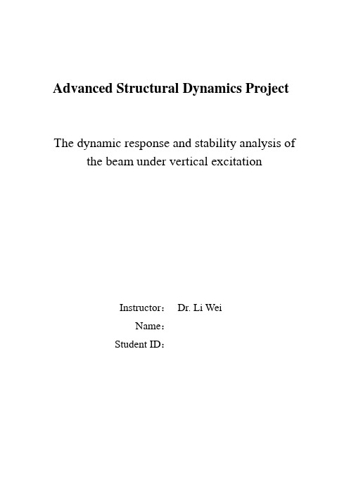
Advanced Structural Dynamics ProjectThe dynamic response and stability analysis of the beam under vertical excitationInstructor:Dr. Li WeiName:Student ID:1.Problem description and the purpose of the project1.1 calculation modelAn Eular beam subjected to an axial force. Please build the differential equation of motion and use a proper difference method to solve this differential equation. Study the dynamic stability of the beam related to the frequency and amplitude of the force. As shown in the Fig 1.1.Fig1.11.2 purpose and process arrangementa.learning how to create mathematical model of the continuoussystem and select proper calculation method to solve it.b.learning how to build beam vibration equation and solve Mathieuequation.ing Floquet theory to judge vibration system’s stability andanalyze the relationship among the frequency and amplitude of the force and dynamic response.This project will introduce the establishment of the mathematical model of the continuous system in section 2, the movement equation and the numerical solution of using MATLAB in section 3, Applying Floquent theory to study the dynamic stability of the beam related to the frequency and amplitude of the force in section 4. In the last of the project, we get some conclusions in section 5.2. the mathematical model of the systemThe geometric model of the beam and force-simplified diagram is shown in Fig.2.1.We assume that its stiffness(EI) is constant and the deflection of the beam is small, and the boundary conditions is simply support. Now the beam subjected to an axial force. We assume the force is equal to 0cos P t ω. F=f 0coswt yxFig.2.1We select the length of x ∆ in any position of the beam, the free-body diagram is shown in Fig.2.2.Fig.2.2Using equations of movement equilibrium, that is to say:+↑()y y F m a ∑=∆ (1)0G M +∑= (2) From equation (1), we will get:22),(),(ty x A t x x S t x S ∂∂∆=∆+-ρ (3)Divide equation (3) by x ∆ and take the limit:22xy A x S ∂∂=∂∂-ρ (4) Then synthesize equation (2),we can get:0),()],(),([),(),(=∆∆+--∆++-∆+x t x x S t x y t x x y F t x M t x x M (5)Divide equation (5) by x ∆ and take the limit:S xy F x M =∂∂+∂∂ (6) Combine equation (4) with (6):0222222=∂∂+∂∂+∂∂ty A x y F x M ρ (7) And 22),(xy EI t x M ∂∂= (8) Combine equation (7) with (8):0)(22222222=∂∂+∂∂+∂∂∂∂ty A x y F x y EI x ρ (9) We know EI is a constant, so0)(222244=∂∂+∂∂+∂∂ty m x y t F x y EI (10) In equation (10), m is the mass of unit length. Now we will use assumed-modes method. Named lx n t T t x y n πsin )(),(=,so: 0sin )(22244422=⎥⎦⎤⎢⎣⎡-+l x n T l n t F T l n EI dt T d m n n n πππ (11) 0))(1(222=-+n non n T F t F P dt T d n=1,2,...... (12) In the equation (12)222222,l EI n F m EI l n P n on ππ==And t F t F ϖcos )(= ,so0)cos 1(222=-+n non n T t F F P dt T d ϖ n=1,2,...... (13) 0)cos (22=-+n n T t dtT d ϖεδ (14) In the equation (12)4)(L n A EI πρδ= 22)(Ln F πε= Equation (14) is the Mathieu equation. it is difficult to solve the analytical solution directly, thus, we use the approximate derivative namely an average acceleration method to get the numerical solution from the reference.3. Numerical solution3.1 using MATLAB to solve equationWe will use the Newmark-β method [1] to solve equation (14). We can use the initial condition 00u u 和to integrate the move equation:m 0u cu ku ++= (15)Fig.3.1As shown in Fig.3.1))(2(11+++∆+=i i i i i u u t u u (16) )(4121+++∆+∆+=i i i i i i i u u t t u u u (17) ()0cos =-+i i u wt u εδ (18)From equation (16), (17) and (18), we will get:()i i u t wn u ∆∆--=∆cos εδ (19)i i ii u u t u 2)2(-∆∆=∆ (20) ()()22]cos [44]cos [)(2tt wn t u t wn u t u i i i ∆∆-+∆+∆-∆-=∆εδεδ (21) When applying the MATLAB, we need discrete the processing time t, get time step 02.0=∆t .When solving the vibration stability interval, there are three variables to participate in the discussion, namely w c ,,δ. So take a particular w first and discuss the remaining two parameters.From Floquent theory [2],we can use parameter A to judge stability.Equation 0)()(22=++y t dt dy t dt y d ξξ(22) Take two sets of special solution:1)0(,0)0(0)0(,1)0(2211====yy yy (20) Parameter [2] )]()([2121T y T y A +=(21) If abs (A) is less than 1, the system is stability. And if abs (A) is greater than 1, the system is instability. When abs(A) is equal to 1, the system is critical state.We use MATLAB Codes to solve equations. We use ω=2 Math ieu Equation to judge the validity of the codes. From Fig.3.2 and Fig.3.3, wecan consider the codes are correct.In these follow figures, ω=2, the horizontal axis is δ, vertical axis is ε.Fig.3.2. stable domain in reference [3]and[2]Fig.3.3. stable domain in MATLAB solutionCompared Fig.3.2 with Fig.3.3, we can see that the stability domain of numerical solutions applying average acceleration method are consistent with the standard solutions. it can concluded that when the system have solution whose cycle is equal to π or 2π, )3,2,1(2 ==n n δThis chapter discusses the accuracy of the vibration stability determination with Floquent theory. The next chapter will discuss the numerical solution and stable domain and two parameters ’ influences on the stability for this question.4. Parameters influenceIn this part, we only consider two parameters, namely the frequency and amplitude of the force.4.1the influence of the force’s frequency4.1.1the stability of the systemWhen we discuss the stability of the system related to the frequency of the force, we should select some different frequencies, so we choose ω=1,2,4,6,8 and10. Using MATLAB codes, we can obtain the figs of the stability. We can know the stable region is bigger with the increase of the frequency in Fig.4.1.ω=1 ω=2ω=4 ω=6ω=8 ω=10Fig.4.1 stable domain with different ω4.1.2the response of the systemWhen we discuss the response of the system, the system should be stable. So we choose 7δ=,1ε=-,ω=2,4 and 6. In Fig.4.2, the cycle of the response increase and the range of the reactive amplitude is smaller with the increase of the frequency.Fig.4.2 responses of the system with different ω4.2the influence of the force’s amplitudeThe εis related to the force’s amplitude P. The cycle of the response a little increase and the range of the reactive amplitude is bigger with the increase of the force’s amplitude, in Fig.4.3.and Fig4.4.Fig.4.3 vibration response curve with different δThe red curve is w=2, δ=12,ε=1; the blue curve is w=2, δ=14, ε=1.This figure state that the vibration cycle is smaller and the amplitude have a little change with the increase of the δ.Fig.4.3 vibration response curve with different εThe red curve is w=2, δ=12,ε=1; the blue curve is w=2, δ=12, ε=5. This figure state that the amplitude is smaller and the vibration cycle have a little change with the increase of the ε.5. Conclusion(1) With the increase of the frequency, the stable region and the cycle of the response are bigger, but the range of the reactive amplitude is smaller.(2)With the incr ease of the force’s amplitude, the cycle of the response a little increase and the range of the reactive amplitude is much bigger. (3)Vibration in the stable region, the vibration cycle is smaller with the increase of the δ; the amplitude is smaller with the increase of the ε.AcknowledgementsThe author is grateful for upperclassman Li Yong, he give me much assistance. And the author is also grateful for Doctor Li Wei. In his classes, I felt very happy and can understand his class effectively. At last, the author is also grateful for classmates in the same laboratory, they give me much guidance and encourage. I gain a lot of knowledge through this study and I will work harder in the future.References1、ROY R.CRSIG, Jr. STRUCTURAL DYNAMICS. New York: John Wiley & Sons.2、王海期. 非线性振动. 北京: 高等教育出版社, 19923、顾志平. 非线性振动. 北京: 中国电力出版社, 2012。
结构动力学大作业1.
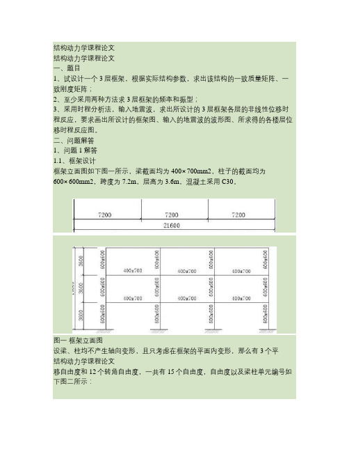
结构动力学课程论文结构动力学课程论文一、题目1、试设计一个3层框架,根据实际结构参数,求出该结构的一致质量矩阵、一致刚度矩阵;2、至少采用两种方法求3层框架的频率和振型;3、采用时程分析法,输入地震波,求出所设计的3层框架各层的非线性位移时程反应,要求画出所设计的框架图、输入的地震波的波形图、所求得的各楼层位移时程反应图。
二、问题解答1、问题1解答1.1、框架设计框架立面图如下图一所示,梁截面均为400⨯700mm2,柱子的截面均为600⨯600mm2,跨度为7.2m,层高为3.6m,混凝土采用C30。
图一框架立面图设梁、柱均不产生轴向变形,且只考虑在框架的平面内变形,那么有3个平结构动力学课程论文移自由度和12个转角自由度,一共有15个自由度,自由度以及梁柱单元编号如下图二所示:V1V2V3图二单元编号及自由度方向先计算各个单元的一致质量矩阵和一致刚度矩阵,然后把相关的单元叠加组合计算得到整个结构的一致质量矩阵和一致刚度矩阵。
1.2、结构的一致质量矩阵梁:=0.4⨯0.7⨯2500=700kg/m, L=7.2m;梁、柱都为均布质量,故:⎧f⎪f⎪⎨⎪f⎪⎩fI1I2I3I4⎫⎪⎪L⎬=420⎪⎪⎭5622L⎡156⎢5415613L⎢⎢22L13L4L⎢⎣-13L-22L-3L-13L⎤-22L⎥⎥-3L⎥⎥4L⎦221⎫⎧v⎪v⎪⎪ 2⎪⎨⎬3⎪⎪v⎪ 4⎪⎩v⎭结构动力学课程论文结构动力学课程论文柱:=0.6⨯0.6⨯2500=900kg/m,L=3.6m 单元刚度矩阵如下:结构动力学课程论文结构动力学课程论文(m)(n)(p)ˆijˆijˆij由mij=m+m+m+....可计算一致质量矩阵中的各元素:(1)(2)(3)(10)(11)(12)(13)ˆ11ˆ11ˆ11ˆ11ˆ11ˆ11ˆ11m11=m+m+m+m+m+m+m=3⨯5040+ 4⨯1203.43=19933.72(10)(11)(12)(13)ˆ12ˆ12ˆ12ˆ12m12=m+m+m+m=4⨯416.57=1666.28结构动力学课程论文m13=0(10)m14=m15=m16=m17=m14=610.97(10)m18=m19=m1,10=m1,11=m18=-361.03 m1,12=m1,13=m1,14=m1,15=0(4)(5)(6)(10)(11)(12)(13)(14)(15)(16)(17)ˆ22ˆ22ˆ22ˆ22ˆ22ˆ22ˆ22ˆ22ˆ22ˆ22ˆ22m22=m+m+m+m+m+m+m+m+m+m+m=3⨯5040+8⨯1203.43=24747.44(14)(15)(16)(17)ˆ23ˆ23ˆ23ˆ23m23=m+m+m+m=4⨯416.57=1666.28(10)m24=m25=m26=m27=m24=361.03(14)(10)ˆ28ˆ28m28=m+m=610.97-610.97=0 同理 m29=m2,10=m2,11=0(14)m2,12=m2,13=m2,14=m2,15=m2.03 ,12=-361(7)(8)(9)(14)(15)(16)(17)(18)(19)(20)(21)ˆ33ˆ33ˆ33ˆ33ˆ33ˆ33ˆ33ˆ33ˆ33ˆ33ˆ33m33=m+m+m+m+m+m+m+m+m+m+m=3⨯5040+8⨯1203.43=24747.44(14)m34=m35=m36=m37=0 m38=m39=m3,10=m3,11=m38=361.03 (14)ˆ3ˆ(18)m3,12=m3,13=m3,14=m3,15=m.97-610.97=0 ,12+m3,12=610(1)(10)(1)ˆ44ˆ44ˆ45m44=m+m=2488.32+399.91=2888.23 m45=m=-1866.24m46=m47=0(10)ˆ48m48=m=-299.93m49=m4,10=m4,11=m4,12=m4,13=m4,14=m4,15=0(2)(1)(2)(11)ˆ56ˆ55ˆ55ˆ55=-1866.24m55=m+m+m=2488.32+2488.32+399.91=5376.55m56=mm57=m58=0(11)ˆ59m59=m=-299.93 m5,10=m5,11=m5,12=m5,13=m5,14=m5,15=0(2)(3)(12)ˆ66ˆ66ˆ66m66=m+m+m=2488.32+2488.32+399.91=5376.55(3)ˆ67m67=m=-1866.24 m68=m69=0(12)ˆ6m6,10=m.93 m6,11=m6,12=m6,13=m6,14=m6,15=0 ,10=-299(3)(13)ˆ77ˆ77m77=m+m=2488.32+399.91=2888.23m78=m79=m7,10=0(13)ˆ7m7,11=m.93 m7,12=m7,13=m7,14=m7,15=0 ,11=-299结构动力学课程论文(4)(10)(14)ˆ88ˆ88ˆ88m88=m+m+m=2488.32+399.91+399.91=3288.14(4)ˆ89m89=m=-1866.24 m8,10=m8,11=0(14)ˆ8m8,12=m.93 m8,13=m8,14=m8,15=0 ,12=-299(4)(5)(11)(15)ˆ99ˆ99ˆ99ˆ99m99=m+m+m+m=2488.32+2488.32+399.91+399.91=5776.46(5)ˆ9m9,10=m.24 ,10=-1866(15)ˆ9.93 m9,14=m9,15=0 m9,11=m9,12=0 m9,13=m,13=-299(5)(6)(12)(16)ˆ10ˆ10ˆ10ˆ10m10,10=m.32+2488.32+399.91+399.91=5776.46 ,10+m,10 +m,10+m,10=2488(6)(16)ˆ10ˆ m10,11=m=-1866.24m=m.93 m10,15=0m=m=010,1210,13,1110,1410,14=-299(6)(13)(17)ˆ11ˆ11ˆ11m11,11=m.32+399.91+399.91=3288.14,11+m,11+m,11=2488m11,12=m11,13=m11,14=0(17)ˆ11m11,15=m.93,15=-299(7)(14)(18)ˆ12ˆ12ˆ12m12,12=m.32+399.91+399.91=3288.14 ,12+m,12+m,12=2488 (7)ˆ12m12,13=m.24 m12,14=m12,15=0 ,13=-1866(7)(8)(15)(19)ˆ13ˆ13ˆ13ˆ13m13,13=m.32+2488.32+399.91+399.91=5776.46 ,13+m,13 +m,13+m,13=2488(8)ˆ13m13,14=m.24 m13,15=0 ,14=-1866(8)(9)(16)(20)ˆ14ˆˆˆm14,14=m+m+m+m.32+2488.32+399.91+399.91=5776.46 ,1414,1 414,1414,14=2488(9)ˆ14m14,15=m.24 ,15=-1866(9)(17)(21)ˆ15ˆ15ˆ15m15,15=m.32+399.91+399.91=3288.14 ,15+m,15+m,15=2488则得:一致质量矩阵(该矩阵为对称矩阵,故下三角省略)单位(kg)结构动力学课程论文0⎡19933.721666.28⎢24747.441666.28⎢⎢24747.44⎢⎢⎢⎢⎢⎢⎢M=⎢⎢⎢⎢⎢⎢⎢⎢⎢⎢⎢⎢⎣610.97361.0302888.23610.97361.030-1866.245376.55610.97361.0300-1866.245376.55610.97361.03000-1866.242888.23-361.030361.03-299.930003288.14-361.030361.030-299.9300-1866.245776.46-361.030361.0300-299.9300-1866.245776.46-361.030361.03000-299.9300-1866.243288.140-361.0300000-299.930003288.14⎤-361.03-361.03-361.03⎥⎥⎥000⎥000⎥⎥000⎥000⎥⎥000⎥000⎥⎥-299.9300⎥⎥0-299.930⎥00-299.93⎥⎥-1866.2400⎥5776.46-1866.240⎥5776.46-1866.24⎥⎥3288.14⎦⎥0001.3、结构的一致刚度矩阵各梁、柱均为等截面,故单元刚度矩阵为:-63L3L⎤⎧v1⎫⎧fs1⎫⎡6⎪f⎪⎪v⎪⎢6-3L-3L⎥⎪s2⎪2EI⎢-6⎪2⎪⎥=⎨⎬⎨⎬ 223⎢⎥f3L-3L2LLL⎪s3⎪⎪v3⎪⎢22⎥⎪⎪f3L-3LL2L⎣⎦⎪⎩v4⎪⎭⎩s4⎭框架梁:C30混凝土E=3⨯107KN/m2,0.40⨯0.73EI=3⨯10⨯=3.43⨯105kN·m2,L=7.2m 127结构动力学课程论文7框架柱:0.60⨯0.603EI=3⨯10⨯=3.24⨯105KN·m2 L=3.6m12结构动力学课程论文结构动力学课程论文结构动力学课程论文ˆ(m)+kˆ(n)+kˆ(p)+....可计算一致刚度矩阵中的各元素:由kij=kijijijˆ(10)+kˆ(11)+kˆ(12)+kˆ(13)=4⨯0.833⨯105=3.332⨯105 k11=k11111111ˆ(10)+kˆ(11)+kˆ(12)+kˆ(13)=4⨯(-0.833k12=k)⨯105=-3.332⨯105 k13=0 12121212 (10)k14=k15=k16=k17=k18=k19=k1,10=k1,11=k14=1.50⨯105k1,12=k1,13=k1,14=k1,15=0ˆ(10)+kˆ(11)+kˆ(12)+kˆ(13)+kˆ(14)+kˆ(15)+kˆ(16)+kˆ(17)=8⨯0.833⨯105=6.664⨯105 k22=k2222222222222222ˆ(14)+kˆ(15)+kˆ(16)+kˆ(17)=4⨯(-0.833k23=k)⨯105=-3.332⨯1052323232310k24=k25=k26=k27=k24=-0.861⨯105ˆ(10)+kˆ(14)=0.861⨯105-0.861⨯105=0 同理 k28=k2828k29=k2,10=k2,11=0结构动力学课程论文ˆ(14)=1.50⨯105 k2,12=k2,13=k2,14=k2,15=k2,12ˆ(14)+kˆ(15)+kˆ(16)+kˆ(17)+kˆ(18)+kˆ(19)+kˆ(20)+kˆ(21)=8⨯0.833⨯105=6.664⨯105 k33=k3333333333333333k34=k35=k36=k37=0(14)k38=k39=k3,10=k3,11=k38=-1.50⨯105ˆ(14)+kˆ(18)=1.50⨯105-1.50⨯105=0 k3,12=k3,13=k3,14=k3,15=k3,123,12ˆ(1)=0.953⨯105 ˆ(1)+kˆ(10)=1.906⨯105+3.60⨯105=5.506⨯105 k=kk44=k44444545 k46=k47=0ˆ(10)=1.80⨯105k48=k48k49=k4,10=k4,11=k4,12=k4,13=k4,14=k4,15=0ˆ(1)+kˆ(2)+kˆ(11)=1.906⨯105+1.906⨯105+3.60⨯105=7.412⨯105k55=k555555ˆ(2)=0.953⨯105 k56=k56k57=k58=0 ˆ(11)=1.80⨯105 k59=k59k5,10=k5,11=k5,12=k5,13=k5,14=k5,15=0ˆ(2)+kˆ(3)+kˆ(12)=1.906⨯105+1.906⨯105+3.60⨯105=7.412⨯105k66=k666666ˆ(3)=0.953⨯105 k67=k67ˆ(12)=1.80⨯105 k=k=k=k=k=0 k68=k69=0 k6,10=k6,116,126,136,146,156,10ˆ(3)+kˆ(13)=1.906⨯105+3.60⨯105=5.506⨯105k77=k7777k78=k79=k7,10=0ˆ(13)=1.80⨯105 k=k=k=k=0 k7,11=k7,127,137,147,157,11ˆ(4)+kˆ(10)+kˆ(14)=1.906⨯105+3.60⨯105+3.60⨯105=9.106⨯105k88=k888888ˆ(4)=0.953⨯105 k89=k89ˆ(14)=1.80⨯105 k=k=k=0 k8,10=k8,11=0 k8,12=k8,138,148,158,12ˆ(4)+kˆ(5)+kˆ(11)+kˆ(15)=1.906⨯105+1.906⨯105+3.60⨯105+3.60⨯105k99=k999999 99=11.012⨯105 14结构动力学课程论文ˆ(5)=0.953⨯105 k9,10=k9,10k9,14=k9,15=0k9,11=k9,12=0ˆ(15)=1.80⨯105 k9,13=k9,13ˆ(5)+kˆ(6)+kˆ(12)+kˆ(16)=1.906⨯105+1.906⨯105+3.60⨯105+3.60⨯105k10,10=k10,1010,1010,1010,10=11.012⨯1055ˆ(6)=0.953⨯105 kˆ(16)k10,11=k10,12=k10,13=0 k10,14=k10,14=1.80⨯10 k10,15=0 10,11ˆ(6)+kˆ(13)+kˆ(17)=1.906⨯105+3.60⨯105+3.60⨯105=9.106⨯105k11,11=k11,1111,1111,11ˆ(17)=1.80⨯105 k11,12=k11,13=k11,14=0 k11,15=k11,15 ˆ(4)+kˆ(7)+kˆ(18)=1.906⨯105+3.60⨯105+3.60⨯105=9.106⨯105k12,12=k12,1212,1212,12ˆ(7)=0.953⨯105 kk12,13=k12,14=k12,15=0 12,13ˆ(7)+kˆ(8)+kˆ(15)+kˆ(19)=1.906⨯105+1.906⨯105+3.60⨯105+3.60⨯105k13,13=k13,1 313,1313,1313,13=11.012⨯105ˆ(8)=0.953⨯105 kk13,14=k13,15=0 13,14ˆ(8)+kˆ(9)+kˆ(16)+kˆ(20)=1.906⨯105+1.906⨯105+3.60⨯105+3.60⨯105k14,14=k14,1 414,1414,1414,14=11.012⨯105ˆ(9)=0.3125⨯105k14,15=k14,15ˆ(9)+kˆ(17)+kˆ(21)=1.906⨯105+3.60⨯105+3.60⨯105=9.106⨯105k15,15=k15,1515,1515,15得到一致刚度矩阵(该矩阵为对称矩阵,故下三角省略)单位(kN/m)⎡3.332⎢⎢⎢⎢⎢⎢⎢⎢⎢⎢K=105⨯⎢⎢⎢⎢⎢⎢⎢⎢⎢⎢⎢⎢⎣-3.3326.6640-3.3326.6641.50-1.5005.5061.50-1.5000.9537.4121.50-1.50000.9537.4121.50-1.500000.9535.5061.500-1.501.800009.1061.500-1.5001.80000.95311.0121.500-1.50001.80000.95311.0121.500-1.500001.80000.9539.10601.50000001.800009.10601.500000001.80000.95311.01201.5000000001.80000.95311.01201.50000000001.80000.9539.106⎤⎥⎥⎥⎥⎥⎥⎥⎥⎥⎥⎥⎥⎥⎥⎥⎥⎥⎥⎥⎥⎥⎥⎦结构动力学课程论文 2 问题2 解答2.1采用振型分解反应谱法,求解框架的频率和振型ˆ}={0}的特征值得到频率ω和振型φ:由[K]-ω2[M]{v在Matlab中导入质量矩阵[M]和刚度矩阵[K],输[v,ω2]=eig(K,M);ω=sqrt(ω2)可得框架的频率为: []ωT={ω1ω2ω3........ω14ω15}={32.861, 109.022, 199.133, 234.897, 299.589, 307.809 , 378.000, 388.414, 454.501, 480.646, 583.896 , 637.664, 747.045, 828.365, 1056.507 }框架的振型为[φ]=[{φ1}{φ2}{φ3}......{φ14}{φ15}]=φ1 φ2 φ3 φ4 φ5 φ6 φ7 φ8φ9 φ10 φ11 φ12 φ13 φ14 φ15结构动力学课程论文2.2 用Stodola法计算三层框架的频率和振型此结构的柔度矩阵是f=K-1=D=fm=⎡52612⎢34661⎢⎢13564⎢⎢-2919⎢-2009⎢⎢-2009⎢-2919⎢10-5⨯⎢-4627⎢-3739⎢⎢-3739⎢⎢-4627⎢-4436⎢⎢-3429⎢-3429⎢⎢⎣-4436453153846316844-648-547-547-648-3237-2622-2622-3237-5313-4034-4034-5313179831712511915-95-55.4-55.4-95-395-408-408-395-2546-1883-1883-2546 1933.61502.4600.3585.14-403.97.9103-69.43-330.8-46.98-141.3-151.2-164.3-169.8-202-2022088.51495.3606.51-631828.14-463.5-16.66-39.22-52.13-197.9-226.6-226.6-114.2-168.9-189.520471488.4605.89-7.983-467.4891.72-635.4-193.6-45.69-344.3-30.81-189.2-169.2-112.1-227.41933.61502.4600.3-69.437.9103-403.9585.14-151.2-141.3-46.98-330.8-202-149.4-169.8-164.3-959-507-53.6-141139.935.2281.15567.3-144114.5114.5109.7-71.595.5537.1-466.3-466.3-74.97214.41-174.8143.1345.392-214.1713.23-171.7134.55129.58-99.996.75140.084-885-466-7545.39143.1-175214.4134.6-172713.2-21440.0896.75-99.9129.6-959.1-507.2-53.6281.15235.225139.93-141.1109.67114.46-143.6567.357.99237.09595.548-71.52-959.1-507.2-53.6281.15235.225139.93-141.1109.67114.46-143.6567.357.99237.09595.548-71.52-768.9-687.5-306.5-28.0246.216-14.4511.743129.09-99.9796.6839.588-186.8664.53-159.7122.14-768.9-687.5-306.511.743-14.4546.216-28.0239.58896.68-99.97129.09122.14-159.7664.53-186.8-898.5⎤-828.5⎥⎥-387.3⎥⎥-1.176⎥7.242⎥⎥-15.89⎥45.168⎥⎥58.04⎥37.49⎥⎥95.943⎥⎥-71.48⎥113.72⎥⎥107.89⎥-127.1⎥⎥525⎥⎦结构动力学课程论文V1(1)=DV1(0)迭代过程列表如下根据D V1(0)⎡52612⎢34661⎢⎢13564⎢⎢-2919⎢-2009⎢⎢-2009⎢-2919⎢10-5⨯⎢-4627⎢-3739⎢⎢-3739⎢⎢-4627⎢-4436⎢⎢-3429⎢-3429⎢⎢-4436⎣453153846316844-648-547-547-648-3237-2622-2622-3237-5313-4034-4034-5313179831712511915-95-55.4-55.4-95-395-408-408-395-2546-1883-1883-2546 1933.61502.4600.3585.14-403.97.9103-69.43-330.8-46.98-141.3-151.2-164.3-169.8-202-2022088.51495.3606.51-631828.14-463.5-16.66-39.22-52.13-197.9-226.6-226.6-114.2-168.9-189.520471488.4605.89-7.983-467.4891.72-635.4-193.6-45.69-344.3-30.81-189.2-169.2-112.1-227.41933.61502.4600.3-69.437.9103-403.9585.14-151.2-141.3-46.98-330.8-202-149.4-169.8-164.3-959-507-53.6-141139.935.2281.15567.3-144114.5114.5109.7-71.595.5537.1-466.3-466.3-74.97214.4-174.8143.145.39-214.1713.2-171.7134.5129.5-99.996.7540.08-885-466-7545.39143.1-175214.4134.6-172713.2-21440.0896.75-99.9129.6-959.1-507.2-53.6281.1535.22139.93-141.1109.67114.46-143.6567.357.9937.0195.54-71.52-959.1-507.2-53.6281.1535.22139.93-141.1109.67114.46-143.6567.357.9937.0995.54-71.52-768.9-768.9-687.5-306.5-28.0246.21-14.4511.74129.1-99.9796.6839.58-186.8664.5-159.7122.14-687.5-306.511.743-14.4546.216-28.0239.58896.68-99.97129.09122.14-159.7664.53-186.8-898.5⎤-828.5-387.3⎥-1.1767.242-15.89⎥45.1658.04⎥37.4995.94⎥-71.48113.7107.8⎥-127.1525⎦⎥⎡1⎤⎢1⎥⎢⎥⎢1⎥⎢⎥⎢1⎥⎢1⎥⎢⎥⎢1⎥⎢1⎥⎢⎥⎢1⎥⎢1⎥⎢⎥⎢1⎥⎢⎥⎢1⎥⎢1⎥⎢⎥⎢1⎥⎢1⎥⎢⎥⎢⎣1⎥⎦V1(1) V1(1) V1(2) V1(2) V1(3) V1(3) V1(4) V1(4 ) V1(5)⎡116889⎤⎢91257.8⎥⎢⎥⎢43091⎥⎢⎥-3558.1⎢⎥⎢-2480.4⎥⎢⎥⎢-2412.9⎥⎢-3571.2⎥⎢⎥-8221.3⎢⎥⎢-6697.9⎥⎢⎥⎢-6710.8⎥⎢⎥-8217.2⎢⎥⎢-12347⎥⎢⎥-9334.2⎢⎥⎢-9331.7⎥⎢⎥⎢⎣-12348⎥⎦10.7810.369-0.03-0.02-0.02-0.03-0.07-0.06-0.06-0.07-0.11-0.08-0.08-0.11949641928321926271926086917330082-3452-2444-2446-3451-7208-5858-5857-7208-9276-7082-7082-9276712580.7504311920.3285-3477-0.037-2465-0.026-2465-0.026-3477-0.037-7335-0.077-5965-0.063-5965-0.063-7335-0.077-9574-0.101-7305-0.077-7305-0.077-9574-0.101693690.7473301840.3252-3454-0.037-2446-0.026-2448-0.026-3454-0.037-7221-0.078-5868-0.063-5868-0.063-7221-0.078-0.1-9304-7103-0.077-7103-0.077-0.1-9304691890.747300910.325-3452-0.04-2444-0.03-2446-0.03-3451-0.04-7209-0.08-5859-0.06-5858-0.06-7209-0.08-9278-0.1-7084-0.08-7084-0.08-9278-0.1则得到第一振型形式为φ1=(-0.1585 -0.1184 -0.0515 0.005910.00418 0.00419 0.00591 0.01234 0.01003 0.01002 0.01234 0.01588 0.01212 0.01212 0.01588)再用公式ω12=(V1)TmV1(0)(V)mV(1)T1(1)1(1),将数据代入得ω1=32.75。
高等结构动力学大作业

高等结构动力学大作业1. 简介高等结构动力学是结构工程学中的一门重要课程,主要研究结构在外力作用下的动力响应。
本次大作业将探讨高等结构动力学的相关内容,包括结构振动、模态分析和地震反应等。
2. 结构振动结构振动是结构动力学的基础知识,是研究结构在外力作用下的运动规律的重要手段。
结构振动可以分为自由振动和受迫振动两种。
2.1 自由振动自由振动是指结构在没有外力作用下的振动。
结构的自由振动可以通过求解结构的固有振型和固有频率来得到。
固有振型是指结构在自由振动时的形态,固有频率是指结构在自由振动时的振动频率。
2.2 受迫振动受迫振动是指结构在外力作用下的振动。
外力可以是周期性的,也可以是非周期性的。
受迫振动可以通过求解结构的响应函数和激励函数来得到。
3. 模态分析模态分析是研究结构振动特性的重要方法,通过模态分析可以得到结构的模态参数,包括模态振型和模态频率。
模态振型是指结构在特定模态下的振动形态,模态频率是指结构在特定模态下的振动频率。
3.1 模态分析的方法常用的模态分析方法包括有限元法、模态超级位置法和模态伸缩法等。
有限元法是一种基于数值计算的方法,通过离散化结构并求解特征值问题来得到结构的模态参数。
模态超级位置法是一种基于振动测量的方法,通过测量结构的振动响应来得到结构的模态参数。
模态伸缩法是一种基于模态参数估计的方法,通过估计结构的模态参数来得到结构的模态参数。
3.2 模态分析的应用模态分析在结构工程中有广泛的应用,包括结构设计、结构优化和结构监测等。
通过模态分析可以评估结构的动力性能,指导结构的设计和优化,以及监测结构的健康状况。
4. 地震反应地震反应是指结构在地震作用下的振动响应。
地震是一种破坏性的外力,对结构的安全性和稳定性具有重要影响。
地震反应分为静力反应和动力反应两种。
4.1 静力反应静力反应是指结构在地震作用下的静态响应。
静力反应可以通过结构的刚度矩阵和地震力谱来计算得到。
静力反应的计算可以采用静力分析和动力分析两种方法。
《结构动力学》结构动力学大作业 研究生课程考核试卷
《结构动力学》结构动力学大作业研究生课程考核试卷研究生课程考核试卷(适用于课程论文、提交报告)科目:结构动力学大作业教师:姓名:学号:专业:岩土工程类别:专硕上课时间: 2015年 9 月至2015 年11 月考生成绩:卷面成绩平时成绩课程综合成绩阅卷评语:阅卷教师 (签名)2重庆大学研究生院制土木工程学院2015级硕士研究生考试试题1 题目及要求1、按规范要求设计一个3跨3层钢筋混凝土平面框架结构(部分要求如附件名单所示;未作规定部分自定)。
根据所设计的结构参数,求该结构的一致质量矩阵、一致刚度矩阵;2、至少采用两种方法求该框架结构的频率和振型;3、输入地震波(地震波要求如附件名单所示),采用时程分析法,利用有限元软件或自编程序求出该框架结构各层的线性位移时程反应。
342 框架设计2.1 初选截面尺寸取所设计框架为3层3跨,跨度均为4.5m ,层高均为3.9m 。
由于基础顶面离室内地面为1m ,故框架平面图中底层层高取 4.9m 。
梁、柱混凝土均采用C30,214.3/c f N mm =,423.010/E N mm =⨯,容重为325/kN m 。
估计梁、柱截面尺寸如下: (1)梁:梁高b h 一般取跨度的11218,取梁高b h =500mm ;5取梁宽300b b mm =;所以梁的截面尺寸为:300500mm mm ⨯ (2)柱:框架柱的截面尺寸根据柱的轴压比限值,按下列公式计算: ①柱组合的轴压力设计值...E N F g n β=其中:β:考虑地震作用组合后柱轴压力增大系数; F :按简支状态计算柱的负荷面积;E g :折算在单位建筑面积上的重力荷载代表值,可近似取为21214/KN m ;n :验算截面以上的楼层层数。
②c N cNA u f ≥其中:N u :框架柱轴压比限值;8度(0.2g ),查抗震规范轴压比限值0.75N u =;cf :混凝土轴心抗压强度设计值,混凝土采用30C ,214.3/cfN mm =。
结构动力学大作业
结构动力学作业姓名:学号:目录1.力插值法 (1)1.1分段常数插值法 (1)1.2分段线性插值法 (4)2.加速度插值法 (7)2.1常加速度法 (7)2.2线加速度法 (9)附录 (12)分段常数插值法源程序 (12)分段线性插值法源程序 (12)常加速度法源程序 (13)线加速度法源程序 (13)1.力插值法力插值法对结构的外荷载进行插值,分为分段常数插值法和分段线性插值法,这两种方法均适用于线性结构的动力反应计算。
1.1分段常数插值法图1-1为一个单自由度无阻尼系统,结构的刚度为k ,质量为m ,位移为y (t ),施加的外力为P (t )。
图1-2为矩形脉冲荷载的示意图,图中t d 表示作用的时间,P 0表示脉冲荷载的大小。
图1-1 单自由度无阻尼系统示意图图1-2 矩形脉冲荷载示意图对于一个满足静止初始条件的无阻尼单自由度体系来说,当施加一个t d 时间的矩形脉冲荷载,此时结构在t d 时间内的位移反应可以用杜哈梅积分得到:0()sin ()2 (1cos )(1cos ) (0)tst st d P y t t d m ty t y t t Tωττωπω=-=-=-≤≤⎰(1-1)如果结构本身有初始的位移和速度,那么叠加上结构自由振动的部分,结构的位移反应为:02()cos sin (1cos) (0)st d y ty t y t t y t t Tπωωω=++-≤≤& (1-2)图1-3 分段常数插值法微段示意图对于施加于结构任意大小的力,将其划分为Δt 的微段,每一段的荷载都为一个常数(每段相当于一个矩形的脉冲荷载),如图1-3所示,则将每一段的位移和速度写成增量的形式为:1cos t sin t (1cos t)iii i y P y y kωωωω+=∆+∆+-∆& (1-3)i+1/sin t cos t sin t iii y P y y kωωωωω=-∆+∆+∆&& (1-4)程序流程图如下i+1cos t sin t (1cos t)iii y P y y kωωωω=∆+∆+-∆i+1/sin t cos t sin ti i i y Py y kωωωωω=-∆+∆+∆图1-4 分段常数插值法流程图根据流程图可以编写相应的算法,利用MATLAB 进行编程,程序源代码见附录。
结构动力学大作业
结构动力学作业姓名:学号:目录1.力插值法 (1)1.1分段常数插值法 (1)1.2分段线性插值法 (4)2.加速度插值法 (7)2.1常加速度法 (7)2.2线加速度法 (9)附录 (12)分段常数插值法源程序 (12)分段线性插值法源程序 (12)常加速度法源程序 (13)线加速度法源程序 (13)1.力插值法力插值法对结构的外荷载进行插值,分为分段常数插值法和分段线性插值法,这两种方法均适用于线性结构的动力反应计算。
1.1分段常数插值法图1-1为一个单自由度无阻尼系统,结构的刚度为k ,质量为m ,位移为y (t ),施加的外力为P (t )。
图1-2为矩形脉冲荷载的示意图,图中t d 表示作用的时间,P 0表示脉冲荷载的大小。
图1-1 单自由度无阻尼系统示意图图1-2 矩形脉冲荷载示意图对于一个满足静止初始条件的无阻尼单自由度体系来说,当施加一个t d 时间的矩形脉冲荷载,此时结构在t d 时间内的位移反应可以用杜哈梅积分得到:0()sin ()2 (1cos )(1cos ) (0)tst st d P y t t d m ty t y t t Tωττωπω=-=-=-≤≤⎰(1-1)如果结构本身有初始的位移和速度,那么叠加上结构自由振动的部分,结构的位移反应为:002()cos sin (1cos) (0)st d yty t y t t y t t Tπωωω=++-≤≤ (1-2)图1-3分段常数插值法微段示意图对于施加于结构任意大小的力,将其划分为Δt 的微段,每一段的荷载都为一个常数(每段相当于一个矩形的脉冲荷载),如图1-3所示,则将每一段的位移和速度写成增量的形式为:1cos t sin t (1cos t)i ii i yP y y kωωωω+=∆+∆+-∆ (1-3)i+1/sin t cos t sin t i ii yP yy kωωωωω=-∆+∆+∆ (1-4)程序流程图如下图1-4分段常数插值法流程图根据流程图可以编写相应的算法,利用MATLAB 进行编程,程序源代码见附录。
结构动力学大作业分析
结构动力学大作业姓名:学号:习题1用缩法减进行瞬态结构动力学分析以确定对有限上升时间得恒定力的动力学响应。
实际结构是一根钢梁支撑着集中质量并承受一个动态荷载。
钢梁长L ,支撑着一个集中质量M 。
这根梁承受着一个上升时间为t τ,最大值为F1的动态荷载F(t)。
梁的质量可以忽略,需确定产生最大位移响应时间max t 及响应max y 。
同时要确定梁中的最大弯曲应力bend σ。
已知:材料特性:25x E E MPa =,质量M =0.03t ,质量阻尼ALPHAD=8; 几何尺寸:L =450mm I=800.64mm h=18mm; 荷载为:F1=20N t τ=0.075s提示:缩减法需定义主自由度。
荷载需三个荷载步(0至加质量,再至0.075s , 最后至1s )ANSYS 命令如下: FINISH/CLE$/CONFIG,NRES,2000 /prep7L=450$H=18 ET,1,BEAM3 ET,2,MASS21,,,4 R,1,1,800.6,18R,2,30 !MASS21的实常数顺序MASSX, MASSY , MASSZ, IXX, IYY , IZZ MP,EX,1,2E5$MP,NUXY ,1,0.3 N,1,0,0,0 N,2,450/2,0,0 N,3,450,0,0E,1,2$E,2,3 !创建单元 TYPE,2$REAL,2 E,2 M,2,UY FINISH/SOLU !进入求解层 ANTYPE,TRANSTRNOPT,REDUCOUTRES,ALL,ALL$DELTIM,0.004 !定义时间积分步长ALPHAD,8 !质量阻尼为8D,1,UY$D,3,UX,,,,,UY !节点1Y方向,约束节点3X、Y方向约束F,2,FY,0LSWRITE,1 !生成荷载步文件1TIME,0.075FDELE,ALL,ALLF,2,FY,20LSWRITE,2 !生成荷载步文件2TIME,1LSWRITE,3 !生成荷载步文件3LSSOLVE,1,3,1 !求解荷载文件1,2,3FINISH/SOLUEXPASS,ON$EXPSOL,,,0.10000 !扩展处理SOLVEFINISH/POST26NUMV AR,0FILE,fdy,rdsp !注意,建立的项目名称为fdy,否则超出最大变量数200,结果无效NSOL,2,2,U,Y,NSOLPLV AR,2 !时间位移曲线PRV AR,2 !得出在0.10000该时间点上跨中位移最大/POST1 !查看某个时刻的计算结果SET,FIRSTPLDISP,1 !系统在0.10000秒时总变形图ETABLE,Imoment,SMISC,6 !单元I点弯矩ETABLE,Jmoment,SMISC,12 !单元J点弯矩ETABLE,Ishear,SMISC,2 !单元I点剪力ETABLE,Jshear,SMISC,8 !单元J点剪力PLLS,IMOMENT,JMOMENT,1,0 !画出弯矩图PLLS,ISHEAR,JSHEAR,,1,0 !画出剪力图结果如下;随着时间位移的大小:可知系统在0.10000秒时总变形最大。
- 1、下载文档前请自行甄别文档内容的完整性,平台不提供额外的编辑、内容补充、找答案等附加服务。
- 2、"仅部分预览"的文档,不可在线预览部分如存在完整性等问题,可反馈申请退款(可完整预览的文档不适用该条件!)。
- 3、如文档侵犯您的权益,请联系客服反馈,我们会尽快为您处理(人工客服工作时间:9:00-18:30)。
Advanced Structural Dynamics ProjectThe dynamic response and stability analysis of the beam under vertical excitationInstructor:Dr. Li WeiName:Student ID:1.Problem description and the purpose of the project1.1 calculation modelAn Eular beam subjected to an axial force. Please build the differential equation of motion and use a proper difference method to solve this differential equation. Study the dynamic stability of the beam related to the frequency and amplitude of the force. As shown in the Fig 1.1.Fig1.11.2 purpose and process arrangementa.learning how to create mathematical model of the continuoussystem and select proper calculation method to solve it.b.learning how to build beam vibration equation and solve Mathieuequation.ing Floquet theory to judge vibration system’s stability andanalyze the relationship among the frequency and amplitude of the force and dynamic response.This project will introduce the establishment of the mathematical model of the continuous system in section 2, the movement equation and the numerical solution of using MATLAB in section 3, Applying Floquent theory to study the dynamic stability of the beam related to the frequency and amplitude of the force in section 4. In the last of the project, we get some conclusions in section 5.2. the mathematical model of the systemThe geometric model of the beam and force-simplified diagram is shown in Fig.2.1.We assume that its stiffness(EI) is constant and the deflection of the beam is small, and the boundary conditions is simply support. Now the beam subjected to an axial force. We assume the force is equal to 0cos P t ω. F=f 0coswt yxFig.2.1We select the length of x ∆ in any position of the beam, the free-body diagram is shown in Fig.2.2.Fig.2.2Using equations of movement equilibrium, that is to say:+↑()y y F m a ∑=∆ (1)0G M +∑= (2) From equation (1), we will get:22),(),(ty x A t x x S t x S ∂∂∆=∆+-ρ (3)Divide equation (3) by x ∆ and take the limit:22xy A x S ∂∂=∂∂-ρ (4) Then synthesize equation (2),we can get:0),()],(),([),(),(=∆∆+--∆++-∆+x t x x S t x y t x x y F t x M t x x M (5)Divide equation (5) by x ∆ and take the limit:S xy F x M =∂∂+∂∂ (6) Combine equation (4) with (6):0222222=∂∂+∂∂+∂∂ty A x y F x M ρ (7) And 22),(xy EI t x M ∂∂= (8) Combine equation (7) with (8):0)(22222222=∂∂+∂∂+∂∂∂∂ty A x y F x y EI x ρ (9) We know EI is a constant, so0)(222244=∂∂+∂∂+∂∂ty m x y t F x y EI (10) In equation (10), m is the mass of unit length. Now we will use assumed-modes method. Named lx n t T t x y n πsin )(),(=,so: 0sin )(22244422=⎥⎦⎤⎢⎣⎡-+l x n T l n t F T l n EI dt T d m n n n πππ (11) 0))(1(222=-+n non n T F t F P dt T d n=1,2,...... (12) In the equation (12)222222,l EI n F m EI l n P n on ππ==And t F t F ϖcos )(= ,so0)cos 1(222=-+n non n T t F F P dt T d ϖ n=1,2,...... (13) 0)cos (22=-+n n T t dtT d ϖεδ (14) In the equation (12)4)(L n A EI πρδ= 22)(Ln F πε= Equation (14) is the Mathieu equation. it is difficult to solve the analytical solution directly, thus, we use the approximate derivative namely an average acceleration method to get the numerical solution from the reference.3. Numerical solution3.1 using MATLAB to solve equationWe will use the Newmark-β method [1] to solve equation (14). We can use the initial condition 00u u 和to integrate the move equation:m 0u cu ku ++= (15)Fig.3.1As shown in Fig.3.1))(2(11+++∆+=i i i i i u u t u u (16) )(4121+++∆+∆+=i i i i i i i u u t t u u u (17) ()0cos =-+i i u wt u εδ (18)From equation (16), (17) and (18), we will get:()i i u t wn u ∆∆--=∆cos εδ (19)i i ii u u t u 2)2(-∆∆=∆ (20) ()()22]cos [44]cos [)(2tt wn t u t wn u t u i i i ∆∆-+∆+∆-∆-=∆εδεδ (21) When applying the MATLAB, we need discrete the processing time t, get time step 02.0=∆t .When solving the vibration stability interval, there are three variables to participate in the discussion, namely w c ,,δ. So take a particular w first and discuss the remaining two parameters.From Floquent theory [2],we can use parameter A to judge stability.Equation 0)()(22=++y t dt dy t dt y d ξξ(22) Take two sets of special solution:1)0(,0)0(0)0(,1)0(2211====yy yy (20) Parameter [2] )]()([2121T y T y A +=(21) If abs (A) is less than 1, the system is stability. And if abs (A) is greater than 1, the system is instability. When abs(A) is equal to 1, the system is critical state.We use MATLAB Codes to solve equations. We use ω=2 Math ieu Equation to judge the validity of the codes. From Fig.3.2 and Fig.3.3, wecan consider the codes are correct.In these follow figures, ω=2, the horizontal axis is δ, vertical axis is ε.Fig.3.2. stable domain in reference [3]and[2]Fig.3.3. stable domain in MATLAB solutionCompared Fig.3.2 with Fig.3.3, we can see that the stability domain of numerical solutions applying average acceleration method are consistent with the standard solutions. it can concluded that when the system have solution whose cycle is equal to π or 2π, )3,2,1(2 ==n n δThis chapter discusses the accuracy of the vibration stability determination with Floquent theory. The next chapter will discuss the numerical solution and stable domain and two parameters ’ influences on the stability for this question.4. Parameters influenceIn this part, we only consider two parameters, namely the frequency and amplitude of the force.4.1the influence of the force’s frequency4.1.1the stability of the systemWhen we discuss the stability of the system related to the frequency of the force, we should select some different frequencies, so we choose ω=1,2,4,6,8 and10. Using MATLAB codes, we can obtain the figs of the stability. We can know the stable region is bigger with the increase of the frequency in Fig.4.1.ω=1 ω=2ω=4 ω=6ω=8 ω=10Fig.4.1 stable domain with different ω4.1.2the response of the systemWhen we discuss the response of the system, the system should be stable. So we choose 7δ=,1ε=-,ω=2,4 and 6. In Fig.4.2, the cycle of the response increase and the range of the reactive amplitude is smaller with the increase of the frequency.Fig.4.2 responses of the system with different ω4.2the influence of the force’s amplitudeThe εis related to the force’s amplitude P. The cycle of the response a little increase and the range of the reactive amplitude is bigger with the increase of the force’s amplitude, in Fig.4.3.and Fig4.4.Fig.4.3 vibration response curve with different δThe red curve is w=2, δ=12,ε=1; the blue curve is w=2, δ=14, ε=1.This figure state that the vibration cycle is smaller and the amplitude have a little change with the increase of the δ.Fig.4.3 vibration response curve with different εThe red curve is w=2, δ=12,ε=1; the blue curve is w=2, δ=12, ε=5. This figure state that the amplitude is smaller and the vibration cycle have a little change with the increase of the ε.5. Conclusion(1) With the increase of the frequency, the stable region and the cycle of the response are bigger, but the range of the reactive amplitude is smaller.(2)With the incr ease of the force’s amplitude, the cycle of the response a little increase and the range of the reactive amplitude is much bigger. (3)Vibration in the stable region, the vibration cycle is smaller with the increase of the δ; the amplitude is smaller with the increase of the ε.AcknowledgementsThe author is grateful for upperclassman Li Yong, he give me much assistance. And the author is also grateful for Doctor Li Wei. In his classes, I felt very happy and can understand his class effectively. At last, the author is also grateful for classmates in the same laboratory, they give me much guidance and encourage. I gain a lot of knowledge through this study and I will work harder in the future.References1、ROY R.CRSIG, Jr. STRUCTURAL DYNAMICS. New York: John Wiley & Sons.2、王海期. 非线性振动. 北京: 高等教育出版社, 19923、顾志平. 非线性振动. 北京: 中国电力出版社, 2012。