To appear in the ACM SIGGRAPH conference proceedings Drag-and-Drop Pasting
Gauge-Gravity Dualities, Dipoles and New Non-Kahler Manifolds

1. Introduction and Summary It is by now clear that the usual way to deal with flux compactifications is to replace the Calabi-Yau SU (n) holonomy condition with an SU (n) or SU (n−p) structure condition, with p being a specific integer [1], [2], [3]. This requires, for example, the existence of two globally defined spinors on the six-dimensional manifold which are everywhere parallel for the SU (3) structures and nowhere parallel for the SU (2) structure (here p = 1). These spinors appear in the supersymmetry transformations of the gravitino and dilatino fields and as a result the supersymmetry conditions drastically restrict the fluxes and the geometry. The restrictions on the geometry are seen in terms of the torsion classes which measure the departure from the Calabi-Yau condition. The SU (3) structure is much more tractable as there are only five torsion classes whereas for the SU (2) structure the torsion decomposes into ninety classes which makes the classification a formidable task [4]. An alternative route by which we retain the properties of SU (n) structures and their consequent classification in terms of torsion classes, yet do not explicitly consider the supersymmetry transformation, is to follow a U-duality map that appears directly from superstring compactifications. The beauty of this approach is that it gives solutions that are explicitly supersymmetric, satisfy the required equations of motion and fall under the classification of torsion classes for SU (n) structure, all in one smooth map. Such an approach was first elucidated in [5], and was later followed in various other works, for 1
The primal-dual method for approximation algorithms and its application to network design p
1
Introduction
Many problems of interest in combinatorial optimization are considered unlikely to have efficient algorithms; most of these problems are N P -hard, and unless P = N P they do not have polynomialtime algorithms to find an optimal solution. Researchers in combinatorial optimization have considered several approaches to deal with N P -hard problems. These approaches fall into one of two classes. The first class contains algorithms that find the optimal solution but do not run in polynomial time. Integer programming is an example of such an approach. Integer programmers attempt to develop branch-and-bound (or branch-and-cut, etc.) algorithms for dealing with particular problems such that the algorithm runs quickly enough in practice for instances of interest, although the algorithm is not guaranteed to be efficient for all instances. The second class contains algorithms that run in polynomial time but do not find the optimal solution for all instances. Heuristics and metaheuristics (such as simulated annealing or genetic algorithms) are one approach in this class. Typically researchers develop a heuristic for a problem and empirically demonstrate its effectiveness on instances of interest. In this survey, we will consider another approach in this second class called approximation algorithms. Approximation algorithms are polynomial-time heuristics for N P -hard problems whose solution values are provably close to optimum for all instances of the problem. More formally, an α-approximation algorithm for an optimization problem is an algorithm that runs in polynomial time and produces a solution whose value is within a factor of α of the value of an optimal solution. The parameter α is called the performance guarantee or the approximation ratio of the algorithm. We assume that the value of any feasible solution is nonnegative for the problems we consider; extensions of the notion of performance guarantee have been developed in other cases, but we will not discuss them here. This survey will follow the convention that α ≥ 1 for minimization problems and α ≤ 1 for maximization problems, so that a 2-approximation algorithm for a minimization problem produces a solution of value no more than twice the optimal value, 1 and a 2 -approximation algorithm for a maximization problem produces a solution of value at least
Advanced Micro Devices, Inc.

To appear in ACM Transactions on Computer SystemsA General Framework for Prefetch Scheduling in Linked Data Structures and its Application to Multi-Chain PrefetchingSEUNGRYUL CHOIUniversity of Maryland,College ParkNICHOLAS KOHOUTEVI Technology LLC.SUMIT PAMNANIAdvanced Micro Devices,Inc.andDONGKEUN KIM and DONALD YEUNGUniversity of Maryland,College ParkThis research was supported in part by NSF Computer Systems Architecture grant CCR-0093110, and in part by NSF CAREER Award CCR-0000988.Author’s address:Seungryul Choi,University of Maryland,Department of Computer Science, College Park,MD20742.Permission to make digital/hard copy of all or part of this material without fee for personal or classroom use provided that the copies are not made or distributed for profit or commercial advantage,the ACM copyright/server notice,the title of the publication,and its date appear,and notice is given that copying is by permission of the ACM,Inc.To copy otherwise,to republish, to post on servers,or to redistribute to lists requires prior specific permission and/or a fee.c 2001ACM1529-3785/2001/0700-0001$5.00ACM Transactions on Computer Systems2·Seungryul Choi et al.Pointer-chasing applications tend to traverse composite data structures consisting of multiple independent pointer chains.While the traversal of any single pointer chain leads to the seri-alization of memory operations,the traversal of independent pointer chains provides a source of memory parallelism.This article investigates exploiting such inter-chain memory parallelism for the purpose of memory latency tolerance,using a technique called multi-chain prefetching. Previous works[Roth et al.1998;Roth and Sohi1999]have proposed prefetching simple pointer-based structures in a multi-chain fashion.However,our work enables multi-chain prefetching for arbitrary data structures composed of lists,trees,and arrays.This article makesfive contributions in the context of multi-chain prefetching.First,we intro-duce a framework for compactly describing LDS traversals,providing the data layout and traversal code work information necessary for prefetching.Second,we present an off-line scheduling algo-rithm for computing a prefetch schedule from the LDS descriptors that overlaps serialized cache misses across separate pointer-chain traversals.Our analysis focuses on static traversals.We also propose using speculation to identify independent pointer chains in dynamic traversals.Third,we propose a hardware prefetch engine that traverses pointer-based data structures and overlaps mul-tiple pointer chains according to the computed prefetch schedule.Fourth,we present a compiler that extracts LDS descriptors via static analysis of the application source code,thus automating multi-chain prefetching.Finally,we conduct an experimental evaluation of compiler-instrumented multi-chain prefetching and compare it against jump pointer prefetching[Luk and Mowry1996], prefetch arrays[Karlsson et al.2000],and predictor-directed stream buffers(PSB)[Sherwood et al. 2000].Our results show compiler-instrumented multi-chain prefetching improves execution time by 40%across six pointer-chasing kernels from the Olden benchmark suite[Rogers et al.1995],and by3%across four pared to jump pointer prefetching and prefetch arrays,multi-chain prefetching achieves34%and11%higher performance for the selected Olden and SPECint2000benchmarks,pared to PSB,multi-chain prefetching achieves 27%higher performance for the selected Olden benchmarks,but PSB outperforms multi-chain prefetching by0.2%for the selected SPECint2000benchmarks.An ideal PSB with an infinite markov predictor achieves comparable performance to multi-chain prefetching,coming within6% across all benchmarks.Finally,speculation can enable multi-chain prefetching for some dynamic traversal codes,but our technique loses its effectiveness when the pointer-chain traversal order is highly dynamic.Categories and Subject Descriptors:B.8.2[Performance and Reliability]:Performance Anal-ysis and Design Aids;B.3.2[Memory Structures]:Design Styles—Cache Memories;C.0[Gen-eral]:Modeling of computer architecture;System Architectures; C.4[Performance of Sys-tems]:Design Studies;D.3.4[Programming Languages]:Processors—CompilersGeneral Terms:Design,Experimentation,PerformanceAdditional Key Words and Phrases:Data Prefetching,Memory parallelism,Pointer Chasing CodeA General Framework for Prefetch Scheduling·3performance platforms.The use of LDSs will likely have a negative impact on memory performance, making many non-numeric applications severely memory-bound on future systems. LDSs can be very large owing to their dynamic heap construction.Consequently, the working sets of codes that use LDSs can easily grow too large tofit in the processor’s cache.In addition,logically adjacent nodes in an LDS may not reside physically close in memory.As a result,traversal of an LDS may lack spatial locality,and thus may not benefit from large cache blocks.The sparse memory access nature of LDS traversal also reduces the effective size of the cache,further increasing cache misses.In the past,researchers have used prefetching to address the performance bot-tlenecks of memory-bound applications.Several techniques have been proposed, including software prefetching techniques[Callahan et al.1991;Klaiber and Levy 1991;Mowry1998;Mowry and Gupta1991],hardware prefetching techniques[Chen and Baer1995;Fu et al.1992;Jouppi1990;Palacharla and Kessler1994],or hybrid techniques[Chen1995;cker Chiueh1994;Temam1996].While such conventional prefetching techniques are highly effective for applications that employ regular data structures(e.g.arrays),these techniques are far less successful for non-numeric ap-plications that make heavy use of LDSs due to memory serialization effects known as the pointer chasing problem.The memory operations performed for array traver-sal can issue in parallel because individual array elements can be referenced inde-pendently.In contrast,the memory operations performed for LDS traversal must dereference a series of pointers,a purely sequential operation.The lack of memory parallelism during LDS traversal prevents conventional prefetching techniques from overlapping cache misses suffered along a pointer chain.Recently,researchers have begun investigating prefetching techniques designed for LDS traversals.These new LDS prefetching techniques address the pointer-chasing problem using several different approaches.Stateless techniques[Luk and Mowry1996;Mehrotra and Harrison1996;Roth et al.1998;Yang and Lebeck2000] prefetch pointer chains sequentially using only the natural pointers belonging to the LDS.Existing stateless techniques do not exploit any memory parallelism at all,or they exploit only limited amounts of memory parallelism.Consequently,they lose their effectiveness when the LDS traversal code contains insufficient work to hide the serialized memory latency[Luk and Mowry1996].A second approach[Karlsson et al.2000;Luk and Mowry1996;Roth and Sohi1999],which we call jump pointer techniques,inserts additional pointers into the LDS to connect non-consecutive link elements.These“jump pointers”allow prefetch instructions to name link elements further down the pointer chain without sequentially traversing the intermediate links,thus creating memory parallelism along a single chain of pointers.Because they create memory parallelism using jump pointers,jump pointer techniques tolerate pointer-chasing cache misses even when the traversal loops contain insufficient work to hide the serialized memory latency.However,jump pointer techniques cannot commence prefetching until the jump pointers have been installed.Furthermore,the jump pointer installation code increases execution time,and the jump pointers themselves contribute additional cache misses.ACM Transactions on Computer Systems4·Seungryul Choi et al.Finally,a third approach consists of prediction-based techniques[Joseph and Grunwald1997;Sherwood et al.2000;Stoutchinin et al.2001].These techniques perform prefetching by predicting the cache-miss address stream,for example us-ing hardware predictors[Joseph and Grunwald1997;Sherwood et al.2000].Early hardware predictors were capable of following striding streams only,but more re-cently,correlation[Charney and Reeves1995]and markov[Joseph and Grunwald 1997]predictors have been proposed that can follow arbitrary streams,thus en-abling prefetching for LDS traversals.Because predictors need not traverse program data structures to generate the prefetch addresses,they avoid the pointer-chasing problem altogether.In addition,for hardware prediction,the techniques are com-pletely transparent since they require no support from the programmer or compiler. However,prediction-based techniques lose their effectiveness when the cache-miss address stream is unpredictable.This article investigates exploiting the natural memory parallelism that exists between independent serialized pointer-chasing traversals,or inter-chain memory parallelism.Our approach,called multi-chain prefetching,issues prefetches along a single chain of pointers sequentially,but aggressively pursues multiple independent pointer chains simultaneously whenever possible.Due to its aggressive exploitation of inter-chain memory parallelism,multi-chain prefetching can tolerate serialized memory latency even when LDS traversal loops have very little work;hence,it can achieve higher performance than previous stateless techniques.Furthermore,multi-chain prefetching does not use jump pointers.As a result,it does not suffer the overheads associated with creating and managing jump pointer state.Andfinally, multi-chain prefetching is an execution-based technique,so it is effective even for programs that exhibit unpredictable cache-miss address streams.The idea of overlapping chained prefetches,which is fundamental to multi-chain prefetching,is not new:both Cooperative Chain Jumping[Roth and Sohi1999]and Dependence-Based Prefetching[Roth et al.1998]already demonstrate that simple “backbone and rib”structures can be prefetched in a multi-chain fashion.However, our work pushes this basic idea to its logical limit,enabling multi-chain prefetching for arbitrary data structures(our approach can exploit inter-chain memory paral-lelism for any data structure composed of lists,trees,and arrays).Furthermore, previous chained prefetching techniques issue prefetches in a greedy fashion.In con-trast,our work provides a formal and systematic method for scheduling prefetches that controls the timing of chained prefetches.By controlling prefetch arrival, multi-chain prefetching can reduce both early and late prefetches which degrade performance compared to previous chained prefetching techniques.In this article,we build upon our original work in multi-chain prefetching[Kohout et al.2001],and make the following contributions:(1)We present an LDS descriptor framework for specifying static LDS traversalsin a compact fashion.Our LDS descriptors contain data layout information and traversal code work information necessary for prefetching.(2)We develop an off-line algorithm for computing an exact prefetch schedulefrom the LDS descriptors that overlaps serialized cache misses across separate pointer-chain traversals.Our algorithm handles static LDS traversals involving either loops or recursion.Furthermore,our algorithm computes a schedule even ACM Transactions on Computer SystemsA General Framework for Prefetch Scheduling·5when the extent of dynamic data structures is unknown.To handle dynamic LDS traversals,we propose using speculation.However,our technique cannot handle codes in which the pointer-chain traversals are highly dynamic.(3)We present the design of a programmable prefetch engine that performs LDStraversal outside of the main CPU,and prefetches the LDS data using our LDS descriptors and the prefetch schedule computed by our scheduling algorithm.We also perform a detailed analysis of the hardware cost of our prefetch engine.(4)We introduce algorithms for extracting LDS descriptors from application sourcecode via static analysis,and implement them in a prototype compiler using the SUIF framework[Hall et al.1996].Our prototype compiler is capable of ex-tracting all the program-level information necessary for multi-chain prefetching fully automatically.(5)Finally,we conduct an experimental evaluation of multi-chain prefetching us-ing several pointer-intensive applications.Our evaluation compares compiler-instrumented multi-chain prefetching against jump pointer prefetching[Luk and Mowry1996;Roth and Sohi1999]and prefetch arrays[Karlsson et al.2000], two jump pointer techniques,as well as predictor-directed stream buffers[Sher-wood et al.2000],an all-hardware prediction-based technique.We also inves-tigate the impact of early prefetch arrival on prefetching performance,and we compare compiler-and manually-instrumented multi-chain prefetching to eval-uate the quality of the instrumentation generated by our compiler.In addition, we characterize the sensitivity of our technique to varying hardware stly,we undertake a preliminary evaluation of speculative multi-chain prefetching to demonstrate its potential in enabling multi-chain prefetching for dynamic LDS traversals.The rest of this article is organized as follows.Section2further explains the essence of multi-chain prefetching.Then,Section3introduces our LDS descriptor framework.Next,Section4describes our scheduling algorithm,Section5discusses our prefetch engine,and Section6presents our compiler for automating multi-chain prefetching.After presenting all our algorithms and techniques,Sections7and8 then report on our experimental methodology and evaluation,respectively.Finally, Section9discusses related work,and Section10concludes the article.2.MULTI-CHAIN PREFETCHINGThis section provides an overview of our multi-chain prefetching technique.Sec-tion2.1presents the idea of exploiting inter-chain memory parallelism.Then, Section2.2discusses the identification of independent pointer chain traversals. 2.1Exploiting Inter-Chain Memory ParallelismThe multi-chain prefetching technique augments a commodity microprocessor with a programmable hardware prefetch engine.During an LDS computation,the prefetch engine performs its own traversal of the LDS in front of the processor,thus prefetching the LDS data.The prefetch engine,however,is capable of traversing multiple pointer chains simultaneously when permitted by the application.Conse-quently,the prefetch engine can tolerate serialized memory latency by overlapping cache misses across independent pointer-chain traversals.ACM Transactions on Computer Systems6·Seungryul Choi et al.<compute>ptr = A[i];ptr = ptr->next;while (ptr) {for (i=0; i < N; i++) {a)b)}<compute>ptr = ptr->next;while (ptr) {}}PD = 2INIT(ID ll);stall stall stallINIT(ID aol);stall stallFig.1.Traversing pointer chains using a prefetch engine.a).Traversal of a single linked list.b).Traversal of an array of lists data structure.To illustrate the idea of exploiting inter-chain memory parallelism,wefirst de-scribe how our prefetch engine traverses a single chain of pointers.Figure1a shows a loop that traverses a linked list of length three.Each loop iteration,denoted by a hashed box,contains w1cycles of work.Before entering the loop,the processor ex-ecutes a prefetch directive,INIT(ID ll),instructing the prefetch engine to initiate traversal of the linked list identified by the ID ll label.If all three link nodes suffer an l-cycle cache miss,the linked list traversal requires3l cycles since the link nodes must be fetched sequentially.Assuming l>w1,the loop alone contains insufficient work to hide the serialized memory latency.As a result,the processor stalls for 3l−2w1cycles.To hide these stalls,the prefetch engine would have to initiate its linked list traversal3l−2w1cycles before the processor traversal.For this reason, we call this delay the pre-traversal time(P T).While a single pointer chain traversal does not provide much opportunity for latency tolerance,pointer chasing computations typically traverse many pointer chains,each of which is often independent.To illustrate how our prefetch engine exploits such independent pointer-chasing traversals,Figure1b shows a doubly nested loop that traverses an array of lists data structure.The outer loop,denoted by a shaded box with w2cycles of work,traverses an array that extracts a head pointer for the inner loop.The inner loop is identical to the loop in Figure1a.In Figure1b,the processor again executes a prefetch directive,INIT(ID aol), causing the prefetch engine to initiate a traversal of the array of lists data structure identified by the ID aol label.As in Figure1a,thefirst linked list is traversed sequentially,and the processor stalls since there is insufficient work to hide the serialized cache misses.However,the prefetch engine then initiates the traversal of subsequent linked lists in a pipelined fashion.If the prefetch engine starts a new traversal every w2cycles,then each linked list traversal will initiate the required P T cycles in advance,thus hiding the excess serialized memory latency across multiple outer loop iterations.The number of outer loop iterations required to overlap each linked list traversal is called the prefetch distance(P D).Notice when P D>1, ACM Transactions on Computer SystemsA General Framework for Prefetch Scheduling·7 the traversals of separate chains overlap,exposing inter-chain memory parallelism despite the fact that each chain is fetched serially.2.2Finding Independent Pointer-Chain TraversalsIn order to exploit inter-chain memory parallelism,it is necessary to identify mul-tiple independent pointer chains so that our prefetch engine can traverse them in parallel and overlap their cache misses,as illustrated in Figure1.An important question is whether such independent pointer-chain traversals can be easily identi-fied.Many applications perform traversals of linked data structures in which the or-der of link node traversal does not depend on runtime data.We call these static traversals.The traversal order of link nodes in a static traversal can be determined a priori via analysis of the code,thus identifying the independent pointer-chain traversals at compile time.In this paper,we present an LDS descriptor frame-work that compactly expresses the LDS traversal order for static traversals.The descriptors in our framework also contain the data layout information used by our prefetch engine to generate the sequence of load and prefetch addresses necessary to perform the LDS traversal at runtime.While compile-time analysis of the code can identify independent pointer chains for static traversals,the same approach does not work for dynamic traversals.In dynamic traversals,the order of pointer-chain traversal is determined at runtime. Consequently,the simultaneous prefetching of independent pointer chains is limited since the chains to prefetch are not known until the traversal order is computed, which may be too late to enable inter-chain overlap.For dynamic traversals,it may be possible to speculate the order of pointer-chain traversal if the order is pre-dictable.In this paper,we focus on static LDS ter in Section8.7,we illustrate the potential for predicting pointer-chain traversal order in dynamic LDS traversals by extending our basic multi-chain prefetching technique with specula-tion.3.LDS DESCRIPTOR FRAMEWORKHaving provided an overview of multi-chain prefetching,we now explore the al-gorithms and hardware underlying its implementation.We begin by introducing a general framework for compactly representing static LDS traversals,which we call the LDS descriptor framework.This framework allows compilers(and pro-grammers)to compactly specify two types of information related to LDS traversal: data structure layout,and traversal code work.The former captures memory refer-ence dependences that occur in an LDS traversal,thus identifying pointer-chasing chains,while the latter quantifies the amount of computation performed as an LDS is traversed.After presenting the LDS descriptor framework,subsequent sections of this article will show how the information provided by the framework is used to perform multi-chain prefetching(Sections4and5),and how the LDS descriptors themselves can be extracted by a compiler(Section6).3.1Data Structure Layout InformationData structure layout is specified using two descriptors,one for arrays and one for linked lists.Figure2presents each descriptor along with a traversal code exampleACM Transactions on Computer Systems8·Seungryul Choi etal.a).b).Bfor (i = 0 ; i < N ; i++) {... = data[i].value;}for (ptr = root ; ptr != NULL; ) { ptr = ptr->next;}Fig.2.Two LDS descriptors used to specify data layout information.a).Array descriptor.b).Linked list descriptor.Each descriptor appears inside a box,and is accompanied by a traversal code example and an illustration of the data structure.and an illustration of the traversed data structure.The array descriptor,shown in Figure 2a,contains three parameters:base (B ),length (L ),and stride (S ).These parameters specify the base address of the array,the number of array elements traversed by the application code,and the stride between consecutive memory ref-erences,respectively.The array descriptor specifies the memory address stream emitted by the processor during a constant-stride array traversal.Figure 2b illus-trates the linked list descriptor which contains three parameters similar to the array descriptor.For the linked list descriptor,the B parameter specifies the root pointer of the list,the L parameter specifies the number of link elements traversed by the application code,and the ∗S parameter specifies the offset from each link element address where the “next”pointer is located.The linked list descriptor specifies the memory address stream emitted by the processor during a linked list traversal.To specify the layout of complex data structures,our framework permits descrip-tor composition.Descriptor composition is represented as a directed graph whose nodes are array or linked list descriptors,and whose edges denote address generation dependences.Two types of composition are allowed.The first type of composition is nested composition .In nested composition,each address generated by an outer descriptor forms the B parameter for multiple instantiations of a dependent inner descriptor.An offset parameter,O ,is specified in place of the inner descriptor’s B parameter to shift its base address by a constant offset.Such nested descriptors cap-ture the memory reference streams of nested loops that traverse multi-dimensional data structures.Figure 3presents several nested descriptors,showing a traversal code example and an illustration of the traversed multi-dimensional data structure along with each nested descriptor.Figure 3a shows the traversal of an array of structures,each structure itself containing an array.The code example’s outer loop traverses the array “node,”ac-cessing the field “value”from each traversed structure,and the inner loop traverses ACM Transactions on Computer SystemsA General Framework for Prefetch Scheduling·9a).b).c).for (i = 0 ; i < L 0 ; i++) {... = node[i].value;for (j = 0 ; j < L 1 ; j++) {... = node[i].data[j];}}for (i = 0 ; i < L 0 ; i++) {down = node[i].pointer;for (j = 0 ; j < L 1 ; j++) {... = down->data[j];}}node for (i = 0 ; i < L 0 ; i++) {for (j = 0 ; j < L 1 ; j++) {... = node[i].data[j];}down = node[i].pointer;for (j = 0 ; j < L 2 ; j++) {... = down->data[j];}}node Fig.3.Nested descriptor composition.a).Nesting without indirection.b).Nesting with indirection.c).Nesting multiple descriptors.Each descriptor composition appears inside a box,and is accompanied by a traversal code example and an illustration of the composite data structure.each embedded array “data.”The outer and inner array descriptors,(B,L 0,S 0)and (O 1,L 1,S 1),represent the address streams produced by the outer and inner loop traversals,respectively.(In the inner descriptor,“O 1”specifies the offset of each inner array from the top of each structure).Figure 3b illustrates another form of descriptor nesting in which indirection is used between nested descriptors.The data structure in Figure 3b is similar to the one in Figure 3a,except the in-ner arrays are allocated separately,and a field from each outer array structure,“node[i].pointer,”points to a structure containing the inner array.Hence,as shown in the code example from Figure 3b,traversal of the inner array requires indirect-ing through the outer array’s pointer to compute the inner array’s base address.In our framework,this indirection is denoted by placing a “*”in front of the inner descriptor.Figure 3c,our last nested descriptor example,illustrates the nestingACM Transactions on Computer Systems10·Seungryul Choi et al.main() { foo(root, depth_limit);}foo(node, depth) { depth = depth - 1; if (depth == 0 || node == NULL)return;foo(node->child[0], depth);foo(node->child[1], depth);foo(node->child[2], depth);}Fig.4.Recursive descriptor composition.The recursive descriptor appears inside a box,and is accompanied by a traversal code example and an illustration of the tree data structure.of multiple inner descriptors underneath a single outer descriptor to represent the address stream produced by nested distributed loops.The code example from Fig-ure 3c shows the two inner loops from Figures 3a-b nested in a distributed fashion inside a common outer loop.In our framework,each one of the multiple inner array descriptors represents the address stream for a single distributed loop,with the order of address generation proceeding from the leftmost to rightmost inner descriptor.It is important to note that while all the descriptors in Figure 3show two nesting levels only,our framework allows an arbitrary nesting depth.This permits describ-ing higher-dimensional LDS traversals,for example loop nests with >2nesting depth.Also,our framework can handle non-recurrent loads using “singleton”de-scriptors.For example,a pointer to a structure may be dereferenced multiple times to access different fields in the structure.Each dereference is a single non-recurrent load.We create a separate descriptor for each non-recurrent load,nest it under-neath its recurrent load’s descriptor,and assign an appropriate offset value,O ,and length value,L =1.In addition to nested composition,our framework also permits recursive compo-sition .Recursively composed descriptors describe depth-first tree traversals.They are similar to nested descriptors,except the dependence edge flows backwards.Since recursive composition introduces cycles into the descriptor graph,our frame-work requires each backwards dependence edge to be annotated with the depth of recursion,D ,to bound the size of the data structure.Figure 4shows a simple recursive descriptor in which the backwards dependence edge originates from and terminates to a single array descriptor.The “L”parameter in the descriptor spec-ifies the fanout of the tree.In our example,L =3,so the traversed data structure is a tertiary tree,as shown in Figure 4.Notice the array descriptor has both B and O parameters–B provides the base address for the first instance of the descriptor,while O provides the offset for all recursively nested instances.In Figures 2and 4,we assume the L parameter for linked lists and the D parame-ter for trees are known a priori,which is generally not ter in Section 4.3,we discuss how our framework handles these unknown descriptor parameters.In addi-ACM Transactions on Computer Systems。
Effect of radiation induced current on the quality of MR images

Effect of radiation induced current on the quality of MR imagesin an integrated linac-MR systemBen Burke a)Department of Physics,University of Alberta,11322–89Avenue,Edmonton,Alberta T6G2G7,Canadaand Department of Oncology,Medical Physics Division,University of Alberta,11560University Avenue,Edmonton,Alberta T6G1Z2,CanadaK.WachowiczDepartment of Medical Physics,Cross Cancer Institute,11560University Avenue,Edmonton,Alberta T6G1Z2,Canada and Department of Oncology,Medical Physics Division,University of Alberta,11560University Avenue,Edmonton,Alberta T6G1Z2,CanadaB.G.FalloneDepartment of Physics,University of Alberta,11322–89Avenue,Edmonton,Alberta T6G2G7,Canada;Department of Medical Physics,Cross Cancer Institute,11560University Avenue,Edmonton,Alberta T6G1Z2,Canada;and Department of Oncology,Medical Physics Division,University of Alberta,11560University Avenue,Edmonton,Alberta T6G1Z2,CanadaSatyapal RatheeDepartment of Medical Physics,Cross Cancer Institute,11560University Avenue,Edmonton,Alberta T6G1Z2,Canada and Department of Oncology,Medical Physics Division,University of Alberta,11560University Avenue,Edmonton,Alberta T6G1Z2,Canada(Received22May2012;revised29August2012;accepted for publication30August2012;published21September2012)Purpose:In integrated linac-MRI systems,the RF coils are exposed to the linac’s pulsed radiation, leading to a measurable radiation induced current(RIC).This work(1)visualizes the RIC in MRI raw data and determines its effect on the MR image signal-to-noise ratio(SNR)(b)examines the effect of linac dose rate on SNR degradations,(c)examines the RIC effect on different MRI sequences,(d)examines the effect of altering the MRI sequence timing on the RIC,and(e)uses a postprocessingmethod to reduce the RIC signal from the MR raw data.Methods:MR images were acquired on the linac-MR prototype system using various imaging se-quences(gradient echo,spin echo,and bSSFP),dose rates(0,50,100,150,200,and250MU/min) and repetition times(TR)with the gradient echo sequence.The images were acquired with the radia-tion beam either directly incident or blocked from the RF coils.The SNR was calculated for each of these scenarios,showing a loss in SNR due to RIC.Finally,a postprocessing method was applied to the image k-space data in order to remove partially the RIC signal and recover some of the lost SNR.Results:The RIC produces visible spikes in the k-space data acquired with the linac’s radiation incident on the RF coils.This RIC leads to a loss in imaging SNR that increases with increasing linac dose rate(15%–18%loss at250MU/min).The SNR loss seen with increasing linac dose rate appears to be largely independent of the MR sequence used.Changing the imaging TR had interesting visual effects on the appearance of RIC in k-space due to the timing between the linac’s pulsing and the MR sequence,but did not change the SNR loss for a given linac dose rate.The use of a postprocessing algorithm was able to remove much of the RIC noise spikes from the MR image k-space data,resulting in the recovery of a significant portion,up to81%(Table II),of the lost image SNR.Conclusions:The presence of RIC in MR RF coils leads to a loss of SNR which is directly related to the linac dose rate.The RIC related loss in SNR is likely to increase for systems that are able to provide larger than250MU/min dose.Some of this SNR loss can be recovered through the use of a postprocessing algorithm,which removes the RIC artefact from the image k-space.©2012American Association of Physicists in Medicine.[/10.1118/1.4752422]Key words:linac-MR,radiation induced currentI.INTRODUCTIONOur research group has integrated a linear accelerator(linac) with a magnetic resonance imaging(MRI)system.1,2This system will provide real-time,intrafractional images3with tu-mor specific contrast to allow significant reductions in mar-gins for the planning target volume.As a result,both im-proved normal tissue sparing and dose escalation to the tu-mor will be possible,which are expected to improve treatment outcomes.The radio frequency(RF)coils used in MR imaging are exposed to the pulsed radiation of the linac in the integrated6139Med.Phys.39(10),October2012©2012Am.Assoc.Phys.Med.61390094-2405/2012/39(10)/6139/9/$30.00linac-MR system.The receive coil will either sit close to or right in contact with the patient.Therefore,there will be beam orientations in a treatment plan where the coil will be irradi-ated.This has been shown to result in instantaneous currents being induced in the MR coils—called radiation induced cur-rent(RIC).4RIC has been widely reported on in various ma-terials when exposed to various sources of radiation.5–9These extraneous currents have the potential to adversely affect MR imaging by distorting the RF signal being measured by the RF coils.Our more recent results have shown that the RIC signal in RF coils can be reduced with the application of ap-propriate buildup material to the coils.10This buildup method was effective with planar or cylindrical coil geometries and was unhindered by the presence of magneticfields.This work explores another method for RIC removal that does not in-volve altering the RF coils,but instead uses image process-ing techniques.Recently published work by Yun et al.dis-cusses the importance of imaging signal-to-noise ratio(SNR) for real-time tumor tracking3and this provides the motivation for the use of a postprocessing algorithm to recover some of the SNR lost due to RIC.Their work showed that the accu-racy of the autocontouring algorithm was reduced when the field strength was reduced from0.5T to0.2T,due to the decrease in contrast-to-noise ratio(CNR).3The measured, average centroid root mean squared error in their tracking algorithm was increased by factors of1.5and2.4,respec-tively,in their spherical and nonspherical phantoms(see Table III in Ref.3).At a givenfield strength,an increase in the image noise due to the RIC noise spikes will reduce both the SNR and the CNR,thus further decreasing the accuracy of the autocontouring and tracking method.At high magnetic fields the RIC artefact may not be of great importance due to the inherently higher SNR.However,performing fast imag-ing,which is required for real-time tracking,at lowfields dic-tates that we are in a SNR challenged environment and as such,any further degradation of SNR is highly undesirable.In this work,we image phantoms in the linac-MR system in the presence of pulsed radiation from the linear accelerator. These experiments clearly demonstrate the presence of RIC in the MRI raw data,i.e.,k-space.The purpose of this work is to (a)visualize the RIC in MRI raw data and determine its effect of the MR image quality,specifically the SNR(b)examine the effect of linac dose rate,in monitor units(MU)per minute,on the SNR degradation caused by the RIC,(c)examine the RIC effect on different MRI sequences,(d)examine the effect of altering the MRI sequence timing,specifically the repetition time(TR),on the visual appearance of the RIC in MRI raw data,and(e)use postprocessing methods to remove the un-wanted RIC signal from the MR images.II.MATERIALS AND METHODSThe linac-MRI system used in these experiments is that de-scribed by Fallone et al.2and shown schematically in Fig.1. The system is comprised of a0.22T biplanar magnet from MRI Tech Co.(Winnipeg,MB,Canada)and a6MV linear accelerator with its beam directed to the imaging volume of the magnet.The x-ray beam direction isperpendicular F IG.1.Schematic diagram on linac-MR system showing the split solenoid MR magnet,the linear accelerator and the rotational gantry.to both the main magneticfield and the superior-inferior orientation of the patient.It should be noted that Fig.1 does not clearly show the RF coil.The B1field in MRI is perpendicular to the main magneticfield.Thus,the axis of the RF coil is either along the patients’head-foot direction or along the radiation beam direction.Moreover,the RF coil sits closer to the patient for the best SNR in the receive signal.The standard RF coils are either cylindrical with axis along the patients’head-foot direction or surface coils resting directly on the patients’skin.In all of these cases,the coil conductor will be directly exposed to the radiation.The maximum gradient strength of the MR system is specified as 40mT/m and the MR system is controlled using a TMX NRC console(National Research Council of Canada,Institute of Biodiagnostics,Winnipeg,MB,Canada).The console software is PYTHON-based[Python Software Foundation, Hampton,NH(Ref.11)]to allow full user control of the development and modification of pulse sequences.Analogic (Analogic Corporation,Peabody,MA)AN8295gradient coil amplifiers and AN81103kW RF power amplifiers are used.The linac components are composed of salvaged parts from a decommissioned magnetron-based Varian600C sys-tem,which include the straight-through waveguide(without bending magnet).The distance of the linac target to the mag-net center is80cm.Presently,the MV x-ray beam has pri-mary collimators and thefinal prototype design will include secondary collimators and the multileaf collimator(MLC).2 As such the radiationfield size was larger than the coils,so the entirety of the RF coils was irradiated during the experi-ments.However,our previous work(Ref.4,Fig.8)has shown that the RIC amplitude increased as the irradiated area of the coil conductor is increased.Two RF coils were used in the imaging experiments.The first was a small,∼3cm diameter solenoid coil with14turns of wire.The tuning and impedance matching of this coil is accomplished by variable capacitances and it contains an in-tegrated pin-diode transmit/receive switch.All active compo-nents are outside the volume of the solenoid such that these can be placed outside the radiation beam.The second coil was a10cm diameter solenoid coil containing5concentricMedical Physics,Vol.39,No.10,October2012rings made of0.64cm diameter copper pipe.The tuning of the coil is accomplished by a variable capacitance while the impedance matching is accomplished with a variable induc-tor.As with the smaller coil,this coil contains an integrated pin-diode transmit/receive switch with the active components residing outside the solenoid volume.Both coils were con-structed by NRC and resonate nominally at the appropriate frequency of9.3MHz for the0.22T MRI.The phantom used in the smaller coil was an acrylic rectan-gular cube,15.95×15.95×25.4mm3,with3holes of diame-ters2.52,3.45,and4.78mm drilled into it.The cube was then placed in a22.5mm diameter tube andfilled with a10mM solution of CuSO4.This arrangementfills the holes in the cube with the CuSO4creating three circular signal regions in the MRI image.2The phantom used in the10cm diam-eter coil consisted of four tubes of27mm diameterfilled with a solution of61.6mM NaCl and7.8mM CuS04. The tubes were stacked into a2×2matrix arrangement and held together with an adhesive tape.This arrange-ment again created four circular signal regions in the MRI image.12II.A.Effect of RIC and linear accelerator dose rateon MR imagesThis experiment was designed to determine the effect of RIC on the SNR in MRI images including the impact of the linac dose rate.A standard gradient echo sequence was used in all experiments.For the phantom in the smaller coil the imaging parameters were as follows:slice thickness–5 mm;acquisition size–512(read)×128(phase);field of view (FOV)–50×50mm2;TR–300ms;echo-time(TE)–35ms;flip angle–60◦;no signal averaging.For the phantom used in the larger coil the imaging parameters were as follows: Slice thickness–3.5mm;acquisition size–256(read)×128 (phase);FOV–100×100mm2;TR–300ms;TE–35ms;flip angle–90◦;no signal averaging.For the small coil,512 points in the read direction was chosen for easy visualization of the RIC artefact;more points in the read direction means a longer acquisition window,which in turn leads to more radia-tion pulses being present during signal acquisition.Images of both phantoms werefirst obtained with the linac not producing radiation.The same imaging was then repeated with the linac producing radiation at50,100,150,200,250 monitor units per minute(MU/min,i.e.,the dose rate).The imaging experiments in the presence of the radiation beam were further divided into two parts.In thefirst experiment, the radiation was directly incident on the RF coils.In the sec-ond experiment,a lead block was placed in the beam path to attenuate completely the radiation from reaching the RF coil. This was done to ensure that any effect seen in the MR im-ages was caused only by the direct irradiation of the coils, resulting in RIC in the coil and not due to any residual RF noise.The residual RF noise,if it exists,will still reach the coil even if the x-ray beam was completely attenuated by the lead block.The method and effect of RF shielding for this system has been previously described.12This means that a total of11(beam off,beam on atfive different dose rates,beam on but blocked at the samefive dose rates)different imaging conditions were examined for each phantom and coil combination.Five images were taken in each condition to assure repro-ducibility and to provide statistical information.The resulting images were then analyzedfirst by calculating the SNR of the image and second,by examining the k-space data associated with each image,using appropriate window and level,to vi-sualize the RIC artefact(see Fig.5).The SNR was calculated by taking the mean of the signal divided by the standard de-viation of the background noise.For each of the11imaging conditions the mean and standard deviation of thefive SNR values were calculated.II.B.Dependence of RIC artefact on imaging sequence The effect of the MR imaging sequence on the RIC arte-fact was examined by repeating the imaging experiments from Sec.II.A,using a spin echo sequence and a balanced steady-state free precession(bSSFP)sequence instead of the gradi-ent echo sequence used in Sec.II.A.The small coil described above was used for both sequences.SNR was calculated as in Sec.II.A.The imaging parameters for the spin echo sequence were: slice thickness–5mm;acquisition size–256(read)×128 (phase);FOV–50×50mm2;TR–300ms;TE–30ms;no signal averaging;flip angle–90◦.The imaging parameters for the bSSFP sequence were:slice thickness–5mm;acqui-sition size–128(read)×128(phase);FOV–50×50mm2; TR–18ms;no signal averaging;flip angle–60◦.II.C.Dependence of RIC artefact on imaging parameter TRThe next imaging experiment was done by keeping the linac dose rate constant at250MU/min and the imaging pa-rameters identical to those in Sec.II.A,except for the repeti-tion time,TR,which was changed.These experiments were only performed with the smaller coil and the gradient echo sequence was used.Images were acquired at TR values of: 299,299.8,299.9,300,300.1,300.2,301,302,303,304,and 305ms.This investigation examined the relationship between the RIC artefact and the MR sequence timing.The SNR and k-space data were again examined.II.D.Removal of RIC artefact from MR data using postprocessingFinally,the software program MATLAB(The MathWorks, Inc.,Natick,MA)was used as a postprocessing tool in an attempt to remove the RIC artefact from the image k-space data and restore some of the SNR lost due to RIC.The algorithm is similar in application to an adaptivefilter used to removed speckle noise from synthetic aperture radar images as discussed by Russ(see Ref.13Chap.3,p.165top),which uses a neighborhood comparison of pixel brightness,with a threshold based on the average and standard deviation,andMedical Physics,Vol.39,No.10,October2012replaces those above the threshold with a weighted averagevalue of the neighborhood.The algorithm searches pixel-by-pixel for anomalous sig-nal spikes in k-space and then removes them.These spikesare found by searching the k-space data for pixels with in-tensities above a global threshold value;the global thresh-old value was the average background plus three standarddeviations.The average background and standard deviationare determined from a group of pixels near the edge of thek-space image(thus ensuring that it is background).Once an anomalous pixel is found,its magnitude is thencompared to the mean pixel magnitude in the local neighbor-hood surrounding the pixel to determine whether the pixelresides in a background region(i.e.,toward the edges ofk-space)or in a signal region(near the center of k-space).If the pixel’s value is larger than the local average(plus3stan-dard deviations)then the anomalous pixel lies in the back-ground regions,otherwise it lies in the signal region.In otherwords,in order for the pixel to be replaced,its intensity has tobe larger than both the global threshold and local average be-fore it is replaced.The number of pixels in the local neighbor-hood used for comparison in this work was the5×5squarecentered on the point of interest.If the algorithm determinesthat the anomalous pixel is in a background region,the pixelvalue is changed to that of the average background.If the al-gorithm instead determines that the anomalous pixel is in asignal region,then no action is taken.It is obvious that this algorithm will not eliminate all RICspikes from the k-space data,as it will not be able to dis-cern between RIC signal and the MR signal near the center ofk-space.However,this may be acceptable as the RIC spikes near the center of k-space have a minimal effect on SNR be-cause the spikes are sparsely distributed compared to the MRsignal.Also,the magnitude of the RIC noise spikes is smallcompared to the MR signal near the center of k-space.TheMR image was reconstructed from the processed k-space data.The SNR was then recalculated and compared to the originalvalues.parison to medianfilteringThe postprocessing algorithm described above is a customscripted algorithm.Standard image processing techniquesmay also be used to remove the RIC spikes in the k-space.Inorder to compare the postprocessing method with the standardtechniques,two common medianfilters were investigated.Amedianfilter sets a pixel to the median value of the pixels inthe user specified neighborhood around it.Thisfilter is widelyused to remove impulse noise,13,14as it will replace pixelswith excessively large or small values with a more“normal”value.First,the standard medianfilter(function“medfilt2”in MATLAB)was applied globally to the k-space.The“symmet-ric”option was used in MATLAB that causes the boundariesof the images to be extended symmetrically to allow thefil-ter to work at the edges of the image.Second,the adaptivemedianfilter as described by Gonzalez and Woods14was alsoinvestigated using the MATLAB implementation“adpmedian”as given in Ref.15.The“symmetric”option is also used in the adaptive medianfilter.The adaptive medianfilter,“adp-median,”contains a condition which will cause the selective replacement of pixels with the local median values.The al-gorithm will determine the minimum and maximum values in the neighborhood of the pixel of interest,and then if the pixel is either larger than the maximum or smaller than the minimum,the medianfilter is applied.However,if the pixel value is between the minimum and the maximum values,then the pixel value remains unaltered.This selective application will effectively remove impulse noise while preserving more of thefine detail in the image.14Typically,medianfilters are applied directly to the MR im-age,and not to the k-space data,as this is where the impulse noise is seen.However,since our postprocessing algorithm is applied to the k-space data,both medianfilters were also ap-plied to the k-space data.To avoid SNR gains related solely to non-RIC related noise reduction,thefilters were applied to all images,whether acquired with or without radiation.The data are then presented as a percentage calculated using Eq.(1): Percentage of non-RIC SNR=100×SNRfilter,radiation incident on coilSNRfilter,beam blockedImagesacquiredat samedose rate,(1)where“percentage of non-RIC SNR”is the percentage of the original SNR,calculated from the MR data with the radiation beam blocked,“SNRfilter,radiation incident on coil”is the SNR calculated after thefilter has been applied to the MR data acquired with the radiation striking the coil,and “SNRfilter,beam blocked”is the SNR calculated after thefilter has been applied to the MR data acquired with the radiation beam blocked.Both MR data sets are acquired with the same linac dose rate.III.RESULTSIII.A.Effect of RIC and linac dose rate on MR images Thefirst three columns of Tables I and II show the SNR values calculated for each imaging condition described in Sec.II.A for the phantoms imaged with the10cm and3cm coils,respectively.When the lead block stops the radiationT ABLE I.SNR for images acquired with10cm coil using a gradient echo sequence.SNR was calculated by taking the mean of the signal in the magni-tude image divided by the standard deviation of the noise in the real image.Linac Radiation Radiation After RIC dose rate beam blocked beam incident noise is (MU/min)by lead block upon MRI RF coil removed 018.2±0.2–5018.0±0.417.7±0.117.9±0.1 10017.8±0.317.4±0.317.8±0.2 15018.2±0.316.9±0.217.3±0.2 20017.8±0.116.5±0.217.2±0.3 25017.8±0.116.2±0.317.0±0.5Medical Physics,Vol.39,No.10,October2012T ABLE II.SNR for images acquired with3cm coil using a gradient echo sequence.SNR was calculated by taking the mean of the signal in the magni-tude image divided by the standard deviation of the noise in the real image.Linac Radiation Radiation After RIC dose rate beam blocked beam incident noise is (MU/min)by lead block upon MRI RF coil removed019.7±0.3–5019.5±0.418.7±0.319.1±0.4 10019.5±0.318.0±0.319.0±0.2 15019.5±0.417.7±0.419.0±0.3 20019.3±0.217.0±0.118.7±0.3 25019.1±0.416.9±0.318.7±0.4from reaching the coil,the SNR stays relatively constant with linac dose rate for both coils;however,when the lead block is removed and the RF coils are irradiated there is a loss in SNR. Furthermore,the loss in SNR increases as the linac dose rate increases.At the maximum dose rate,250MU/min,Table I shows a decrease in SNR from18.2to16.2when compared to the no radiation scenario,representing an11%loss,or a decrease from17.8to16.2(9%loss)when compared to the radiation blocked scenario at the same dose rate.At the same 250MU/min dose rate,Table II shows a decrease in SNR from19.7to16.9(14%loss)when compared to the no ra-diation scenario,or a decrease from19.1to16.9(11.5%loss) when compared to the radiation blocked scenario at the same dose rate.A graphical representation of the data in Table II is shown in Fig.2.The other objective of the experiments described in Sec.II.A was to visualize the RIC artefact.As mentioned above,the k-space data were examined to accomplish this goal.To illustrate the need to examine the k-space data rather than the image itself we can look to Figs.3and4.The two images shown in Figs.3and4were taken with the10cm and3cm solenoid coil,respectively,with linac dose rates of0 and250MU/min.Visual inspection alone does not show any artefact due to RIC,although the previous analysis shows a loss in SNR.Figure5shows the k-space datacorresponding F IG.2.Signal-to-noise ratio loss due to RIC in3cm solenoid coil.The solid line shows the SNR when the radiation beam is blocked,the dotted line shows the SNR loss when the radiation beam is incident on the RF coil,and the dashed line shows the SNR after the use of a postprocessingalgorithm.F IG.3.Sample images acquired with10cm solenoid coil.The images were acquired with the linac not producing radiation(left)and with linac producing radiation and RF coil unblocked at250MU/min(right).The RIC artefact is not visible.to the images in Fig.4.In the top panel,the k-space with-out radiation is shown.In the bottom panel,the k-space data are shown for the case when the linac producing radiation at 250MU/min that reaches the coil unattenuated.The middle panel shows the k-space data from an image taken with a 250MU/min dose rate where the beam was blocked from reaching the RF coil.Each k-space image has the same win-dow and level applied for consistency.Here the RIC artefact is clearly visible in the k-space data of the image taken with a 250MU/min linac dose rate,but is not visible in the other two k-space data sets.It is clearly based on Fig.5that the vertical lines in k-space are due to the RIC as they are only present when the linac is producing radiation and its beam is incident on the RF coil.III.B.Dependence of RIC artefact on imaging sequenceTables III and IV contain the calculate SNR values for the imaging experiments using a spin echo and bSSFP sequences, respectively.Again when the radiation beam is stopped by a lead block the SNR remains essentially constant at all linac dose rates.When the radiation beam is incident on the RF coil, there is a loss in SNR that increases with increasing dose rate. At the maximum dose rate,250MU/min,Table III shows a decrease in SNR from19.8to16.3(18%loss)when compared to both the no radiation scenario and the radiation blocked scenario at the same dose rate.At the same250MU/min dose rate,Table IV shows a decrease in SNR from20.2to16.5 (18%loss)when compared to the no radiation scenario,ora F IG.4.Sample images acquired with3cm solenoid coil.The images were acquired with the linac not producing radiation(left)and with linac producing radiation and RF coil unblocked at250MU/min(right).The RIC artefact is not visible.Medical Physics,Vol.39,No.10,October2012F IG.5.k-space data from images acquired with linac dose rates of0and 250MU/min.The top image was acquired with the radiation not pulsing. The middle image was acquired with a linac dose rate of250MU/min but the radiation beam was blocked from reaching the coil;it shows no RIC effects. The bottom image was acquired with a linac dose rate of250MU/min and the radiation beam incident on the RF coil;it clearly shows the RIC artefact, which presents itself as near vertical lines in k-space.decrease from19.9to16.5(17%loss)when compared to the radiation blocked scenario at the same dose rate.III.C.Dependence of RIC artefact on imaging parameter TRThe set of imaging experiments described in Sec.II.C was designed to see differences in the RIC artefact,visible in k-space,when the imaging repetition time,TR,was changed. It should be stressed that the loss of SNR as a function of dose rate remained unaltered for all values of TR investigated. Figure6shows some representative images of the k-space data for the TR values specified in Sec.II.C.It is immedi-T ABLE III.SNR for images acquired with3cm coil using a spin echo se-quence.SNR was calculated by taking the mean of the signal in the magni-tude image divided by the standard deviation of the noise in the real image.Linac Radiation Radiation After RIC dose rate beam blocked beam incident noise is (MU/min)by lead block upon MRI RF coil removed019.8±0.3–5019.9±0.319.2±0.619.8±0.4 10019.7±0.217.9±0.619.3±0.4 15019.6±0.417.4±0.519.0±0.6 20019.4±0.416.7±0.718.8±0.3 25019.8±0.316.3±0.518.7±0.4T ABLE IV.SNR for images acquired with3cm coil using a bSSFP sequence. SNR was calculated by taking the mean of the signal in the magnitude image divided by the standard deviation of the noise in the real image.Linac Radiation Radiation After RIC dose rate beam blocked beam incident noise is (MU/min)by lead block upon MRI RF coil removed020.2±0.8–5020.1±0.719.6±0.220.1±0.3 10019.8±0.719.4±0.420.3±0.6 15020.1±0.518.5±0.619.6±0.8 20020.0±0.516.9±0.718.0±1.1 25019.9±0.616.5±0.417.8±0.5ately obvious that even a small change,0.1or0.2ms,in TR results in a large change in the k-space distribution of the RIC artefact.If the TR is changed from300to299.8or300.1ms, the slope of the lines seen in k-space changes dramatically and more lines are seen;12lines are seen in top image of Fig.6(TR–300ms),while14are seen in the middle image (TR–300.1ms).When the TR is changed by larger amounts (i.e.,1ms and up)the RIC appears as randombackground F IG.6.k-space data for gradient echo images taken with the3cm solenoid coil with TR=300,300.1,and301ms with a linac dose rate of250 MU/min and the radiation beam incident on the RF coil.In the top image,TR =300ms,the linac pulses an integer number(54)of times during this TR so the lines seen in k-space due to RIC are nearly vertical.In the middle im-age,TR=300.1ms,there is no longer an integer number of linac pulses during this TR,resulting in timing shifts between successive horizontal(read encode)lines in k-space.Therefore,the lines seen in k-space due to RIC are now slanted from left to right.In the bottom image,TR=301ms,the shift between RIC noise pixels in subsequent horizontal(read encode)lines in k-space is now so large that the RIC artefact appears to be random;however, closer inspection shows that it is still regularly spaced on each read encode line.Medical Physics,Vol.39,No.10,October2012。
空间变化模糊性分析
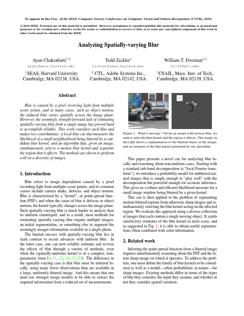
When the blur is spatially-uniform, one has the good fortune of being able to accumulate evidence across the entire image plane, and as a result, one can afford to consider a very general class of blur kernels. In this context, a variety of recent techniques have shown that it is possible to recover completely non-parametric (i.e., tabulated) blur kernels, such as those induced by camera shake, from as little as one image [4, 11, 12, 14, 17, 20]. One general insight that is drawn from this work is that instead of simultaneously estimating the blur kernel and a single sharp image that best explain a given input, it is often preferable to first estimate the blur kernel as that which is most likely under a distribution of sharp images. Levin et al. [17] refer to this process as “MAPk estimation”, and we will use it here. Blur caused by motion or defocus often varies spatially in an image, and in these cases, one must infer the blur kernels using local evidence alone. To succeed at this task, most methods consider a reduced family of blur kernels (e.g., one-dimensional box filters), and they incorporate more input than a single image. When two or more images are available, one can exploit the differences between blur and sensor noise [22] or the required consistency between blur and apparent motion [1, 2, 5, 6] or blur and depth [9, 10]. As an alternative to using two or more images, one can use a single image but assume that a solution to the foreground/background matting problem is given as input [7, 8, 13]. Finally, one may be able to use a single image, but with special capture conditions to exaggerate the effect of the blur, as is done in [16] with a coded aperture (and additional user input) for estimating defocus blur that varies spatially with scene depth. More related to our work is the pioneering effort of Levin [15], who also considers single- image input without pre-matting. The idea is to segment an image into blurred and non-blurred regions and to estimate the PSFs by exploit differences in the distribution of intensity gradients within the two types of regions. These relatively simple image statistics allow compelling results in some cases, but they fail dramatically in others. One of the primary motivations of our work is to understand these failures and to develop stronger computational tools to eliminate them.
Improved results for a memory allocation problem
a rXiv:cs /06121v1[cs.D S]2Dec26Improved results for a memory allocation problem Leah Epstein ∗Rob van Stee †February 1,2008Abstract We consider a memory allocation problem that can be modeled as a version of bin packing where items may be split,but each bin may contain at most two (parts of)items.A 3/2-approximation algorithm and an NP-hardness proof for this problem was given by Chung et al.[3].We give a simpler 3/2-approximation algorithm for it which is in fact an online algorithm.This algorithm also has good performance for the more general case where each bin may contain at most k parts of items.We show that this general case is also strongly NP-hard.Additionally,we give an efficient 7/5-approximation algorithm.1Introduction A problem that occurs in parallel processing is allocating the available memory to the processors.This needs to be done in such a way that each processor has sufficient memory and not too much memory is being wasted.If processors have memory requirements that vary wildly over time,any memory allocation where a single memory can only be accessed by one processor will be inefficient.A solution to this problem is to allow memory sharing between processors.However,if there is a single shared memory for all the processors,there will be much contention which is also undesirable.It is currently infeasible to build a large,fast shared memory and in practice,such memories are time-multiplexed.For n processors,this increases the effective memory access time by a factor of n .Chung et al.[3]studied this problem and described the drawbacks of the methods given above.Moreover,they suggested a new architecture where each memory may be accessed by at most two processors,avoiding the disadvantages of the two extreme earlier models.They abstract the memory allocation problem as a bin packing problem,where the bins are the memories and the items to be packed represent the memory requirements of the processors.This means that the items may be of any size (in particular,they can be larger than 1,which is the size of a bin),and an item may be split,but each bin may contain at most two parts of items.The authors of [3]give a 3/2-approximation for this problem.We continue the study of this problem and also consider a generalized problem where items can still be split arbitrarily,but each bin can contain up to k parts of items,for a given value of k ≥2.We study approximation algorithms in terms of the absolute approximation ratio or the absolute performance guarantee .Let B (I )(or B ,if the input I is clear from the context),be the cost of algorithm B on the input I .An algorithm A is an R -approximation (with respect to the absolute approximation ratio)if for every input I ,A (I )≤R ·OPT (σ),where OPT is an optimal algorithm for the problem.The absolute approximation ratio of an algorithm is the infimum value of R such that the algorithm isan R-approximation.The asymptotic approximation ratio for an online algorithm A is defined to beR∞A=lim supn→∞supIA(I)2unless P=NP.However,since in our problem items can be split,but cannot be packed more than a given number ofparts to a bin,this reduction is not valid.In[3],the authors show that the problem they study is NP-hardin the strong sense for k=2.They use a reduction from the3-P ARTITION problem(see problem[SP15]in[6]).Their result does not seem to imply any consequences with respect to hardness of approximation.We show that the problem is in fact NP-hard in the strong sense for anyfixed value of k.A related,easier problem is known as bin packing with cardinality constraints.In this problem,all items have size at most1as in regular bin packing,and the items cannot be split,however thereis an upper bound of k on the amount of items that can be packed into a single bin.This problemwas studied with respect to the asymptotic approximation ratio.It was introduced and studied in anoffline environment as early as1975by Krause,Shen and Schwetman[9,10].They showed that theperformance guarantee of the well known FIRST FIT algorithm is at most2.7−1252≈1.41421for k=2and mentioned that the lower bounds of[12,11]for the classic problem hold for cardinality constrained bin packing as well.The lower bound of1.5givenby Yao[12]holds for small values of k>2and the lower bound of1.5401given by Van Vliet[11]holds for sufficiently large k.No other lower bounds are known.Finally,Epstein[4]gave an optimalonline bounded space algorithm(i.e.,an algorithm which can have a constant number of active bins atevery time)for this problem.Its asymptotic worst-case ratio is an increasing function of k and tends to1+h∞≈2.69103,where h∞is the best possible performance guarantee of an online bounded space al-gorithm for regular bin packing(without cardinality constraints).Additionally,she improved the onlineupper bounds for3≤k≤6.In particular,the upper bound for k=3was improved to74<s i<Bpartition of the numbers into m sets of size3such that the sum of elements of each set is exactly B.The 3-Partition problem is known to be NP-hard in the strong sense.Given such an instance of the3-Partition problem we define an instance of the splittable item packing with cardinality constraints as follows.There are m(k−3)items,all of size3k−13kB(for k=3we define the size to be s j3k each(the sum is1for k=3).Each bin is packed with k−3padding items and one such triple,giving m sets of k items,each set of sum exactly1.If there is a packing into exactly m bins,as noted above,no items are split and each bin must contain exactly k items.If k=3,this implies the existence of a partition.Consider the case k≥4.Wefirst prove that each bin contains exactly k−3padding items.If a bin contains at least k−2padding items,their total size is at least(3k−1)(k−2)3k2−9k= 1+2k+26k(ℓ≥4).The total sizeis therefore at most(3k−1)(k−ℓ)6k=6k2−2k−5ℓk−ℓ6k(k−3)=1−4(k+1)3k .The original sum of such three items is B,we get that a solution in m binsimplies a partition. 3The NEXT FIT AlgorithmWe can define NEXT FIT for the current problem as follows.This is a straightforward generalization of the standard NEXT FIT algorithm.An item is placed(partially)in the current bin if the bin is not full and the bin contains less than k item parts so far.If the item does notfit entirely in the current bin,the current bin isfilled,closed,and as many new bins are opened as necessary to contain the item.Note that this is an online algorithm.The absolute approximation ratio of NEXT FIT for the classical bin packing problem is2,as Johnson[7]showed.Surprisingly,its approximation ratio for our problem tends to this value for large k.The two problems are different,and the two results seem to be unrelated.Since items may be split,and we consider the absolute approximation ratio,this is the only reason-able online algorithm that can be used for the problem.We show that the approximation ratio of NEXT FIT is exactly2−1/k.Thus,this extremely simple algorithm performs as well as the algorithm from[3] for k=2,and also provides thefirst upper bound for larger values of k.Theorem2The approximation ratio of NEXT FIT is2−1/k.Proof Wefirst show a lower bound.The instance contains an item of size Mk−1followed by M(k−1)k items of sizeε,where M is large andε=1/(Mk(k−1)).Then thefirst item occupies Mk−1bins,and the rest of the items are k per bin,in M(k−1)bins.OPT has Mk bins in total.This proves a lower bound of(M(2k−1)−1)/(Mk),which tends to2−1/k for M→∞.Now we show a matching upper bound.Let u1,u2,...,u m be sizes of the the blocks1,...,m of NF.In each block,all bins are full except perhaps the last one,which contains k parts of items(except for block m,perhaps).We assign weights3to items.Let the size of item i be s i.Then w i=⌈s i⌉/k.Note that in any packing,there are at least⌈s i⌉parts of item i.Since there can be at most k parts in a bin,this meansOPT≥1k.(1)This explains our definition of the weights.This generalizes the weight definition from Chung et al.[3].Consider the last bin from a block i<m.Since NF started a new bin after this bin,it contains kparts of items.Thus it contains at least k−1items of weight1/k(the last k−1items are not split by thealgorithm).If u i=1,there are k such items.If u i>1,consider all items excluding the k−1last items in the last bin.We do not know how many items there are in thefirst u i−1bins(where the last item extends into bin u i).However,for afixed size s,the weight of a group of items of total size s is minimized ifthere is a single item in the group(since we round up the size for each individual item to get the weight).This implies the total weight in a block of u i bins is at least u i/k+(k−1)/k=(u i+k−1)/k.Now consider block m.If u i=1,the weight is at least1/k since there is at least one item.Else,as above the weight is at least u i/k,since the last bin of this block has at least one item or a part of an item. We have NF= u i.ThereforeOPT≥ i w i≥ m i=1(u i+k−1)−(k−1)k.(2)Also by size,OPT>NF−m and thus OPT≥NF−m+1.Multiply this inequality by(k−1)/k and add it(2)to get2k−1k +k−1k−(m−1)k−1Thus we can remove one neighbor from s.We can continue in this way until s has only one neighborleft. Lemma4.2An item of size in((i−1)/2,i/2]has at most i neighbors for all i≥2.Proof Denote the items of size in((i−1)/2,i/2]by type i items.We can consider the items one byone in each tree of the forest.Consider a tree with at least one type i item for some i>1that has at least i+1neighbors.Wewant to create edges between its neighbors and remove edges from the item to the neighbors.However,these neighbors may be type i items themselves,or some other type j≥1.We root the tree at an arbitrary item.Let the type of this item be i.On this item we apply theprocedure detailed below.After doing this,the item has an edge to at most i other items.We definelevels in the tree in the natural way.Level1contains the root,level2now contains at most i items.Wedo not change any edges going up from a particular level.The items in level2undergoes the same procedure if necessary.That is,if the number of its neigh-bors is larger than its type.Afterwards,it only has i neighbors,one of which is on level1.The otherneighbors have moved to some lower level.The procedure to remove a single neighbor of a type i item is as follows.For each item,we applythis procedure until it has at most i outgoing edges.Consider a type i item x which is connected to atleast i+1other items(generally:at least i downlevel items).Say part m j of item x is with part w j ofsome other item in bin j for j=1,...,i′where i′>i.If we are not dealing with the root of the tree, let w i′be the uplevel node.We sort thefirst i′−1≥i bins of this set in order of nondecreasing size of m j.Since the total size of item x is at most i/2,we then have m1+m2≤1.These two parts can thus be put together in one bin.This means cutting one of the neighbors into two and moving it downlevel.We can do this as long as the item has more than i neighbors.5A7/5-approximation for k=2Let k=2.We call items of size in(1/2,1]medium and remaining items large.Our algorithm works as follows.We present it here in a simplified form which ignores the fact that it might run out of small items in the middle of step2(b)or while packing a large item in step4.We will show later how to deal with these cases while maintaining an approximation ratio of7/5.See Figure1.We begin by giving an example which shows that this algorithm is not optimal.For some integer N, consider the input which consists of4N small items of size2/N,2N medium items of size1−1/N, 3N medium items of size1−2/N.ALG packs the items of size1−1/N in4N bins,together with4N small items.It needs3N(1−2/N)=3N−6bins for the remaining medium items.Thus it needs7N−6bins in total.OPT places3N small items in separate bins(one per bin),and N small items are split into two equal parts.This gives5N bins in which there is exactly enough room to place all the medium items. Theorem3This algorithm achieves an absolute approximation ratio of7/5.The analysis has three cases,depending on whether the algorithm halts in step3,5or6.The easiest case among these is without a doubt step5,at least as long as all bins packed in step5contain two small items.5.1Algorithm halts in step5Based on inequality(1),we define weights as follows.51.Sort the small items in order of increasing size,the medium items in order of decreasing size,and the large items in order of decreasing size.2.Pack the medium items one by one,as follows,until you run out of medium or small items.(a)If the current itemfits with the smallest unpacked small item,pack them into a bin.(b)Else,pack the current item together with the two largest small items in two bins.3.If no small items remain unpacked,pack remaining medium and large items using Next Fit andhalt.Start with the medium items.4.Pack all remaining small items in separate bins.Pack the large items one by one into these binsusing Next Fit(starting with the largest large item and smallest small item).5.If any bins remain that have only one small item,repack these small items in pairs into binsand halt.6.Pack remaining large items using Next Fit.Figure1:The approximation algorithm for k=2Definition1The weight of an item of size w i is⌈w i⌉/2.In our proofs,we will also use weights of parts of items,based on considering the total weight of an item and the number of its parts.By Definition1,small and medium items have weight1/2.Therefore, we have the following bounds on total weight of bins packed in the different steps:2.(a)1/2+1/2=12.(b)We pack three items of weight1/2in two bins,or3/4weight per bin on average.4.Consider a large item which is packed in g bins,that is,together with in total g small items.Itssize is strictly larger than g−12≤ni=1W i≤OPT.(3) 6Specifically,we will have W i≥⌈w i⌉/2for i=1,...,n.Thus the numbers W i will generate a better lower bound for OPT,that we can use to show a better upper bound for our algorithm.This is the central idea of our analysis.We initialize W i=⌈w i⌉/2for i=1,...,n.There are four cases.Case1OPT packs x by itself.In this case we give x adjusted weight1,and so our algorithm packs an adjusted weight of1in each of the(two)bins that contain x.Case2OPT packs x with part of a small item.Again x and the bins with x get an adjusted weight of 1.This holds because when OPT splits a small item(or a medium item),it is as if it packs two small items,both of weight1/2.Therefore such an item gets adjusted weight1.We can transfer the extra1/2 from the small item to x.Case3OPT combines x with a complete small item y.Since our algorithm starts by considering the smallest small items,y must have been packed earlier by our algorithm,i.e.with a larger medium item x′(which is not critical!).If OPT packs x′alone or with part of a small item,it has an adjusted weight of1(Cases1and2).Thus the bin with x′has an adjusted weight of3/2,and we transfer1/2to x. If OPT packs x′with a full small item y′,then y′is packed with a larger non-critical item x′′by our algorithm,etc.Eventually wefind a non-critical medium item x∗which OPT packs alone or with part of a small item,or for which Case4holds.The difference between the weight and the adjusted weight of x∗will be transferred to x.Note that the bin in which our algorithm packs x∗has a weight of1since x∗is non-critical.All intermediate items x′,x′′,...have weight1/2and are non-critical as well,and we change nothing about those items.Case4OPT packs x with a split medium or large item,or splits x itself.Since there might be several critical items for which Case4holds,we need to consider how OPT packs all these items to determine their adjusted weight.We are going to allocate adjusted weights to items according to the following rules:1.Each part of a small item(in the OPT packing)gets adjusted weight1/2.2.A part of a large item which is in a bin by itself gets adjusted weight1.3.A part of a large item which is combined with some other item gets adjusted weight1/2.We do not change the weight of non-critical items.The critical items receive an adjusted weight which corresponds to the number of bins that they occupy in the packing of OPT.As noted above,this packing consists of trees and loops.Loops were treated in Case1.To determine the adjusted weights,we consider the non-medium items that are cut into parts by OPT.Each part of such an item is considered to be a single item for this calculation and has adjusted weights as explained above.We then have that the optimal packing consists only of trees with small and medium items,and loops.It can be seen that each part of a non-medium item(for instance,part of a large item)which is in a tree has weight1/2.Consider a tree T in the optimal packing.Denote the number of edges(bins)in it by t.Since all items in T are small or medium,there are t+1items(nodes)in T by Lemmas4.1and4.2.Any items that are small(or part of a small item)or medium but non-critical have adjusted weight equal to the weight of a regular small or medium item which is1/2.Denoting the number of critical items in T by c,wefind that the t+1−c non-critical items have weight t+1−c2)/c=12cwhile still satisfying(3).This expression is minimized by taking c maximal,c=t+1,and is then t/(t+1).We can therefore assign an adjusted weight of t/(t+1)to each critical item in T.7Since the algorithm combines a critical item with two small items of weight (at least)1/2,it packs a weight of 1+t/(t +1)=2t +12t +2per bin.This ratio is minimized for t =2and is 5/6.However,let us consider the case t =2in more detail.If the OPT tree with item x (which is now a chain of length 2)consists of three critical items,then the sum of sizes of these items is at most 2.Our algorithm packs each of these items with two small items which do not fit with one such item.Let the sizes of the three medium items be m 1,m 2,m 3.Let the two small items packed with m i be s i,j for j =1,2.We have that m 1+m 2+m 3≤2but m i +s i,j >1for i =1,2,3and j =1,2.Summing up the last six inequalities and subtracting the one before,we get that the total size of all nine items is at least 4.Thus the area guarantee in these six bins is at least 2/3.If one of the items in the chain is (a part of)a small or large item,or a medium non-critical item,it has adjusted weight 1/2.This leaves an adjusted weight of 3/4for the other two items.In this case we pack at least 3/4+1=7/4in two bins,or 7/8per bin.For t ≥3,we also find a minimum ratio of 7/8.Thus we can divide the bins with critical items into two subtypes:A with an adjusted weight of 5/6and area 2/3,and B with an adjusted weight of (at least)7/8and area 1/2.5.3Algorithm halts in step 3We divide the bins that our algorithm generates into types.We have1.groups of two small items and one medium item in two bins2.pairs of one small item and one medium item in one bin3.groups of four or more medium items in three or more bins4.groups of three medium items in two bins5.one group of bins with 0or more medium items and all the large itemsNote that bins of type 4contain a total weight of at least 3/4(3/2per two bins),as well as a total size of at least 3/4(3items of size more than 1/2in two bins).Thus,whether we look at sizes or at weights,it is clear that these bins can be ignored if we try to show a ratio larger than 4/3.Furthermore,in the bins of type 5we ignore that some of the items may be medium.The bounds that we derive for the total size and weight packed into these bins still hold if some of the items are only medium-sized.The bins of type 1contain the critical items.We say the bins with subtype A are of type 1a ,and the bins with subtype B are of type 1b .Define x 1a ,x 1b,x 2,x 3,x 4as the number of bins with types 1a,1b,2,3,and 5,respectively.Consider the bins of type 3.Let k be the number of groups of medium items.Let t i ≥3be the number of bins in group 1≤i ≤k .The items in group i have total size more than t i −1/2,since the last bin contains a complete medium item.The total weight of a group is t i +12.We get that the total size of items in bins of type 3is at least k i =1(t i −12,and the total weight of these items is k i =1t i +12.We find two different lower bounds on OPT.Adjusted weight:OP T ≥58x 1b +x 2+x 32+x 53x 1a +x 1b2+x 3−kMultiplying thefirst inequality by45we get715x1a+x1b+1110+25max(x5−1,0).(6)If x5=0we are done.Else,(5)is strict and we getOP T>22+x22+x5−1.(7)This means x3and x5occur with the same fractions in(4)and(7).Thus we can set x3:=x3+x5and x5:=0.Adding(4)and(7)and dividing by2givesOPT>316x1b−14x1b+14.Clearly,this holds if any of x1a,x2or x3areat least14.Finally,by(4)we are also done if58x1b+x2+x32≥542x1a+97x2+k14x3.Since we may assume x3<14,we are in particular done if x1b≥18or k≥6.This leaves a limited set of options for the values of x1a,x1b,x2,x3and k that need to be checked. It is possible to verify that for almost all combinations,wefind OPT≥57ALG is possible.If x2=1and x5=2,a packing into twobins could exist in case there is only one large item.(If the bins counted in x5contain two medium items,then we have that the three medium items require(at least)two bins and the small item requires an extra bin.)If such a packing exists,it works as follows:packfirst the medium item,then the large item(partially in the second bin),then the small item.If this gives a packing into two bins,this is how our algorithm packs the items.Otherwise we already have an optimal packing.If x1b=4,x2=1and x5=5,it is a simple matter to try all possible packings for the items in7 bins and check if one is valid.(We can try all possible forests on at most13nodes and at most7edges.) If there is no packing in7bins,then our algorithm maintains the ratio of7/5.If there is one,we use it.5.4Algorithm halts in step6In this case we have the following bin types.1.groups of two small items and one medium item in two bins92.pairs of one small item and one medium item in one bin3.groups of large items with small items4.one group of large itemsBy definition,the type 1bins contain the critical items.We again make a distinction between type 1a bins with subtype A and type 1b bins with subtype B .In type 2bins,the weight is 1.Consider a large item which occupies 2bins of type 3.This item has weight of 1and is combined with two small items in two bins,giving a weight of 1per bin.The large item also has size more than 1,so an area of at least 1/2is packed per paring this to type 1b bins,which have a weight guarantee of only 7/8but also an area guarantee of 1/2,we find that we may assume there are no such type 3bins (with a large item occupying two bins).Now consider a large item which occupies 4bins of type 3.Now we find an overall weight of at least 3,as well as an overall size of at least 3(since the large item did not fit with 3small items in 3bins).Since we plan to show a ratio larger than 4/3,we can ignore such bins as well.This also holds for large items that occupy g ≥5bins:the weight of the large item is at least g/4if g is even and at least (g +1)/4if g is odd.We may therefore assume that all bins of type 3form groups of three bins,containing a weight of at least 5/2and an area of at least 2.This gives a weight of 5/6per bin and an area of 2/3per bin,just like type 1a .We denote the number of type 1b items by x 1and the number of type 1a and 3items by x 3.Adjusted weight:OPT ≥76x 3+x 4/2.(8)Size:OPT ≥13x 2+27OPT ≥x 1+615x 3+25max(x 4−1,0).If x 4=0,we are done.Otherwise,we are done if 115x 3≥34(x 3+x 4)≥52.This holds in particular if x 4≥14.Finally,from (8)we get that we are done if 914x 4,implying that we are done if x 1≥4a pair only needs10/7if we want to show an approximation ratio of7/5.Bins in step5which contain a pair of small items have weight1.Thus if some items are packed in step2(a)or5(as a pair),we can transfer1/4of adjusted weight to the bin with only one small item.If a pair of bins is packed in step2(b),we can transfer5/21of adjusted weight to the bin with the small item,which then has more than5/7of adjusted weight.The only case left is where some bins are packed in step4,and one bin in step5(with one item).If there is a large item which is packed into an odd number g of bins,the weight of it is at least(g+1)/4 and we are again done since we can transfer1/4.If g is even and at least4,the weight is g/4.If g=2,the weight of the large item is1and wefind a weight of1per bin.So we may assume g≥4for all groups.This means that all groups have an area guarantee of at least3/4.Suppose all large items are packed into even numbers of bins.Denoting the total number of bins that we pack by b,wefind that b is odd(since there is exactly one bin with only one small item)and that b is equal to the number of small items that we pack.The weight packed into these bins is at least (b−1)/4+b/2.If4|b−1,this implies(b−1)/4+(b+1)/2bins are needed by OPT,which is more than3b/4.If4∤b−1,there is at least one group of size6or more.In this case we work with area guarantees: the area guarantee in a group of size6is5,and wefind an area guarantee of5for this group plus the lone bin with one small item,or an area guarantee of5/7per bin.(The remaining groups all have area guarantee of at least3/4.)This concludes the proof of Theorem3.6ConclusionsIn this paper,we gave thefirst upper bounds for general k for this problem.Furthermore we provided an efficient algorithm for k=2.An interesting question is whether it is possible to give an efficient algorithm with a better approximation ratio for k=2or for larger k.In a forthcoming paper[5]we will present approximation schemes for these problems.However,these schemes are less efficient than the algorithms given in this paper already forǫ=2/5.References[1]Luitpold Babel,Bo Chen,Hans Kellerer,and Vladimir Kotov.Algorithms for on-line bin-packingproblems with cardinality constraints.Discrete Applied Mathematics,143(1-3):238–251,2004. [2]Alberto Caprara,Hans Kellerer,and Ulrich Pferschy.Approximation schemes for ordered vectorpacking problems.Naval Research Logistics,92:58–69,2003.[3]Fan Chung,Ronald Graham,Jia Mao,and George Varghese.Parallelism versus memory allocationin pipelined router forwarding engines.Theory of Computing Systems,39(6):829–849,2006. [4]Leah Epstein.Online bin packing with cardinality constraints.In Proc.of the13th Eur.Symp.Alg.(ESA2005),pages604–615,2005.To appear in SIAM Journal on Discrete Mathematics.[5]Leah Epstein and Rob van Stee.Approximation schemes for packing splittable items with cardi-nality constraints.Manuscript.[6]M.R.Garey and puters and Intractability:A Guide to the theory of NP-Completeness.W.H.Freeman and Company,New York,1979.[7]David S.Johnson.Fast algorithms for bin packing.Journal of Computer and System Sciences,8(3):272–314,1974.11[8]Hans Kellerer and Ulrich Pferschy.Cardinality constrained bin-packing problems.Annals ofOperations Research,92:335–348,1999.[9]K.L.Krause,V.Y.Shen,and Herbert D.Schwetman.Analysis of several task-scheduling algo-rithms for a model of multiprogramming computer systems.Journal of the ACM,22(4):522–550, 1975.[10]K.L.Krause,V.Y.Shen,and Herbert D.Schwetman.Errata:“Analysis of several task-schedulingalgorithms for a model of multiprogramming computer systems”.Journal of the ACM,24(3):527–527,1977.[11]Andr´e van Vliet.An improved lower bound for online bin packing rmation Pro-cessing Letters,43(5):277–284,1992.[12]Andrew C.C.Yao.New algorithms for bin packing.Journal of the ACM,27:207–227,1980.12。
数字通信(第四版)部分习题答案
Problem 4.11 : (a) As an orthonormal set of basis functions we consider the set f1 (t) = f3 (t) = 1 0≤t<1 0 o.w 1 2≤t<3 0 o.w
f2 (t) = f4 (t) =
2 2 2
|s1 − s2 |2 =
4 −2 −2 −1
2
=
25
= = =
√ √ √
5 12
14 √ 2 −3 3 3 −2 |s2 − s4 |2 = = 31 d2,4 = √ 2 0 1 3 −3 |s3 − s4 |2 = = 19 d3,4 = √ Thus, the minimum distance between any pair of vectors is dmin = 5.
⇒
(b) For non-independent information sequence the power spectrum of s(t) is given by : Φss (f ) =
1 T
|G(f )|2 Φbb (f ). But : φbb (m) = E [bn+m bn ] = E [a a ] + kE [an+m−1 an ] + kE [an+m an−1 ] + k 2 E [an+m−1 an−1 ] n+m n 2 m=0 1+k , k, m = ±1 = 0, o.w.
1 + k2 , m=0 k, m = ±4 ⇒ Φbb (f ) = 1 + k 2 + 2k cos 2πf 4T φbb (m) = 0, o.w.
The Copula-GARCH model of conditional dependencies, An international stock market application
The Copula-GARCH model of conditionaldependencies:An international stockmarket applicationEric Jondeau,Michael Rockinger *Swiss Finance Institute and University of Lausanne,Lausanne,SwitzerlandAbstractModeling the dependency between stock market returns is a difficult task when returns follow a com-plicated dynamics.When returns are non-normal,it is often simply impossible to specify the multivariate distribution relating two or more return series.In this context,we propose a new methodology based on copula functions,which consists in estimating first the univariate distributions and then the joining distri-bution.In such a context,the dependency parameter can easily be rendered conditional and time varying.We apply this methodology to the daily returns of four major stock markets.Our results suggest that con-ditional dependency depends on past realizations for European market pairs only.For these markets,de-pendency is found to be more widely affected when returns move in the same direction than when they move in opposite directions.Modeling the dynamics of the dependency parameter also suggests that de-pendency is higher and more persistent between European stock markets.Ó2006Published by Elsevier Ltd.JEL classification:C51;F37;G11Keywords:Stock indices;International correlation;Dependency;GARCH model;Skewed Student-t distribution;Copula function*Corresponding author.University of Lausanne,Ecole des HEC,Department of Finance and Insurance,1015Lausanne,Switzerland.Tel.:þ41216923348;fax:þ41216923435.E-mail addresses:eric.jondeau@unil.ch (E.Jondeau),michael.rockinger@unil.ch (M.Rockinger).0261-5606/$-see front matter Ó2006Published by Elsevier Ltd.doi:10.1016/j.jimonfin.2006.04.007Journal of International Money and Finance 25(2006)827e853828 E.Jondeau,M.Rockinger/Journal of International Money and Finance25(2006)827e8531.IntroductionAn abundant literature has investigated how the correlation between stock market returns varies when markets become agitated.In a multivariate GARCH framework,for instance, Hamao et al.(1990),Susmel and Engle(1994),and Bekaert and Harvey(1995)have measured the interdependence of returns and volatilities across stock markets.More specifically,Longin and Solnik(1995)have tested the hypothesis of a constant conditional correlation between a large number of stock markets.They found that correlation generally increases in periods of high-volatility of the U.S.market.In addition,in a similar context,tests of a constant cor-relation have been proposed by Bera and Kim(2002)and Tse(2000).Recent contributions by Kroner and Ng(1998),Engle and Sheppard(2001),Engle(2002),and Tse and Tsui(2002) have developed GARCH models with time-varying covariances or correlations.As an alterna-tive approach,Ramchand and Susmel(1998)and Ang and Bekaert(2002)have estimated a mul-tivariate Markov-switching model and tested the hypothesis of a constant international conditional correlation between stock markets.They obtained that correlation is generally higher in the high-volatility regime than in the low-volatility regime.In this context,an important issue is how dependency between stock markets can be mea-sured when returns are non-normal.In the GARCH framework,some recent papers have focused on multivariate distributions which allow for asymmetry as well as fat tails.For instance,multivariate skewed distributions,and in particular the skewed Student-t distribution, have been studied by Sahu et al.(2001)and Bauwens and Laurent(2002).In addition,in the Markov-switching context,Chesnay and Jondeau(2001)have tested for a constant correlation between stock returns,while allowing for Student-t innovations.1For most types of univariate distributions,however,it is simply impossible to specify a multivariate extension that would allow the dependency structure to be captured.In this paper,we present a new methodology to measure conditional dependency in a GARCH context.Our methodology builds on so-called ‘‘copula’’functions.These functions provide an interesting tool to model a multivariate distri-bution when only marginal distributions are known.Such an approach is,thus,particularly use-ful in situations where multivariate normality does not hold.An additional interesting feature of copulas is the ease with which the associated dependency parameter can be conditioned and rendered time varying,even when complicated marginal dynamics are estimated.We use this methodology to investigate the impact of certain joint stock return realizations on the subsequent dependency of international markets.Many univariate models have been pro-posed to specify the dynamics of returns.However,given the focus of this work,we draw on recent advances in the modeling of conditional returns that allow second,third,and fourth moments to vary over time.Our univariate model builds on Hansen’s(1994)seminal paper. In that paper,a so-called skewed Student-t distribution is derived.This distribution allows for a control of asymmetry and fat-tailedness.By rendering these characteristics conditional, it is possible to obtain time-varying higher moments.2This model,therefore,extends Engle’s (1982)ARCH and Bollerslev’s(1986)GARCH models.In an extension to Hansen(1994), 1Some papers also considered how correlation varies when stock market indices are simultaneously affected by very large(positive or negative)fluctuations.Longin and Solnik(2001),using extreme value theory,found that dependency increases more during downside movements than during upside movements.Poon et al.(2004)adopted an alternative statistical framework to test conditional dependency between extreme returns and showed that such a tail dependency may have been overstated once the time-variability of volatility is accounted for.2Higher moments refer to the standardized third and fourth central moments.Jondeau and Rockinger (2003a,b)determine the expression of skewness and kurtosis of the skewed Student-t distribution and show how the cumulative distribution function (cdf)and its inverse can be computed.They show how to simulate data distributed as a skewed Stu-dent-t distribution and discuss how to parametrize time-varying higher moments.We then consider two alternative copula functions which have different characteristics in terms of tail dependency:the Gaussian copula that does not allow any dependency in the tails of the distribution,and the Student-t copula that is able to capture such a tail dependency.Fi-nally,we propose several ways to condition the dependency parameter with past realizations.It is thus possible to test several hypotheses of the way in which dependency varies during turbu-lent periods.In the empirical part of the paper,we investigate the dependency structure between daily returns of major stock market indices over 20years.As a preliminary step,we provide evidence that the skewed Student-t distribution with time-varying higher moments fits very well the uni-variate behavior of the data.Then,we check that the Student-t copula is able to capture the de-pendency structure between market returns.Further scrutiny of the data reveals that the dependency between European markets increases,subsequent to movements in the same direc-tion,either positively or negatively.Furthermore,the strong persistence in the dynamics of the dependency structure is found to reflect a shift,over the sample period,in the dependency pa-rameter.This parameter has increased from about 0.3over the 1980s to about 0.6over the next decade.Such a pattern is not found to hold for the dependency structure between the U.S.mar-ket and the European markets.The remainder of the paper is organized as follows.In Section 2,we first introduce our uni-variate model which allows for volatility,skewness,and kurtosis,to vary over time.In Section 3,we introduce copula functions and describe the copulas used in the empirical application.We also describe how the dependency parameter may vary over time.In Section 4,we present the data and discuss our empirical results.Section 5summarizes our results and concludes.2.A model for the marginal distributionsIt is well known that the residuals obtained from a GARCH model are generally non-normal.This observation has led to the introduction of fat-tailed distributions for innovations.For in-stance,Nelson (1991)considered the generalized error distribution,while Bollerslev and Wool-dridge (1992)focused on Student-t innovations.Engle and Gonzalez-Rivera (1991)modeled residuals non-parametrically.Even though these contributions recognize the fact that errors have fat tails,they generally do not render higher moments time varying,i.e.,parameters of the error distribution are assumed to be constant over time.Our margin model builds on Hansen (1994).2.1.Hansen’s skewed Student-t distributionHansen (1994)was the first to propose a GARCH model,in which the first four mo-ments are conditional and time varying.For the conditional mean and volatility,he built on the usual GARCH model.To control higher moments,he constructed a new density with which he modeled the GARCH residuals.The new density is a generalization of the Student-t distribution while maintaining the assumption of a zero mean and unit vari-ance.The conditioning is obtained by defining parameters as functions of past realizations.829E.Jondeau,M.Rockinger /Journal of International Money and Finance 25(2006)827e 853Some extensions to this seminal contribution may be found in Theodossiou(1998)and Jondeau and Rockinger(2003a).3Hansen’s skewed Student-t distribution is defined bydðz;h;lÞ¼8>>><>>>:bc1þ1hÀ2bzþa1Àl2 À½ðhþ1Þ=2if z<Àa=bbc1þ1bzþa 2 À½ðhþ1Þ=2if z!Àa=b;ð1Þwherea h4l c hÀ2;b2h1þ3l2Àa2;c hGhþ12ffiffiffiffiffiffiffiffiffiffiffiffiffiffiffiffiffiffipðhÀ2ÞpGh2;and h and l denote the degree-of-freedom parameter and the asymmetry parameter,respec-tively.If a random variable Z has the density d(z;h,l),we will write Z w ST(h,l).Additional useful results are provided in the Appendix A.In particular,we characterize the domain of definition for the distribution parameters h and l,give formulas relating higher moments to h and l,and we describe how the cdf of Hansen’s skewed Student-t distribution can be computed.This computation is necessary for the evaluation of the likelihood of the copula function.2.2.A GARCH model with conditional skewness and kurtosisLet the returns of a given asset be given by{r t},t¼1,.,T.Hansen’s margin model with time-varying volatility,skewness,and kurtosis,is defined byr t¼m tþ3t;ð2Þ3t¼s t z t;ð3Þs2 t ¼a0þbþÀ3þtÀ1Á2þbÀÀ3ÀtÀ1Á2þc0s2tÀ1;ð4Þz t w STðh t;l tÞ:ð5ÞEq.(2)decomposes the return of time t into a conditional mean,m t,and an innovation,3t. The conditional mean is modeled with10lags of r t and day-of-the-week dummies.Eq.(3) then defines this innovation as the product between conditional volatility,s t,and a residual, z t.Eq.(4)determines the dynamics of volatility.We use the notation3þt¼maxð3t;0Þand3Àt ¼maxðÀ3t;0Þ.For positivity and stationarity of the volatility process to be guaranteed,parameters are assumed to satisfy the following constraints:a0>0,bþ0;bÀ;c0!0,and3Harvey and Siddique(1999)have proposed an alternative specification,based on a non-central Student-t distribu-tion,in which higher moments also vary over time.This distribution is designed so that skewness depends on the non-centrality parameter and the degree-of-freedom parameter.Note also that the specification of the skewed Student-t distribution adopted by Lambert and Laurent(2002)corresponds to the distribution proposed by Hansen,but with asymmetry parametrized in a different way.830 E.Jondeau,M.Rockinger/Journal of International Money and Finance25(2006)827e853c 0þÀb þ0þb À0Á 2<1.Such a specification has been suggested by Glosten et al.(1993).Eq.(5)specifies that residuals follow a skewed Student-t distribution with time-varying parameters h t and l t .Many specifications could be used to describe the dynamics of h t and l t .To ensure that they remain within their authorized range,we consider an unrestricted dynamic that we constrain via a logistic map.4The type of functional specification that should be retained is discussed in Jon-deau and Rockinger (2003a).The general unrestricted model that we estimate is given by~h t ¼a 1þb þ13þt À1þb À13Àt À1þc 1~ht À1ð6Þ~l t ¼a 2þb þ23þt À1þb À23Àt À1þc 2~l t À1:ð7ÞWe map this dynamic into the authorized domain with h t ¼g L h ;U h ½ð~h t Þand l t ¼g L l ;U l ½ð~l t Þ.Several encompassing restrictions of this general specification are tested in the empirical section of the paper.In particular,we test,within the class of GARCH models of volatility,the following restrictions:a Gaussian conditional distribution,a standard Student-t distribution,and a skewed Student-t distribution with constant skewness and kurtosis.We will see that the most general model cannot be rejected for all the stock indices considered.3.Copula distribution functions3.1.The copula functionConsider two random variables X 1and X 2with marginal cdfs F i (x i )¼Pr[X i x i ],i ¼1,2.The joint cdf is denoted H (x 1,x 2)¼Pr[X 1 x 1,X 2 x 2].All cdfs F i ($)and H ($,$)range in the interval [0,1].In some cases,a multivariate distribution exists,so that the function H ($,$)has an explicit expression.One such case is the multivariate normal distribution.In many cases,however,the margins F i ($)are relatively easy to describe,while an explicit expression of the joint distribution H ($,$)may be difficult to obtain.5In such a context,copulas can be used to link margins into a multivariate distribution func-tion.The copula function extends the concept of multivariate distribution for random variables which are defined over [0,1].This property allows to define a multivariate distribution in terms of margins F i (x i )instead of realizations x i .Then,as highlighted in Sklar’s theorem (see the Appendix A ),one has the equality between the cdf H defined over realizations of the random variables x i and the copula function C defined over margins F i (x i ),so that H (x 1,x 2)¼C (F 1(x 1),F 2(x 2)).We now describe the two copula functions used in our empirical application.For notational convenience,set u i h F i (x i ).The Gaussian copula is defined by the cdfC ðu 1;u 2;r Þ¼F r ÀF À1ðu 1Þ;F À1ðu 2ÞÁ;and the density by4The logistic map,g L ;U ½ðx Þ¼L þðU ÀL Þð1þe Àx ÞÀ1maps R into the interval ]L ,U [.In practice,we use the bounds L h ¼2,U h ¼30for h and L l ¼À1,U l ¼1for l .5It may be argued that multivariate extensions of the skewed Student-t distribution exist (see,in particular,Bauwens and Laurent,2002).In fact,the difficulty comes in this case from the joint estimation of two or more distributions,each involving a large number of unknown parameters.831E.Jondeau,M.Rockinger /Journal of International Money and Finance 25(2006)827e 853cðu1;u2;rÞ¼1ffiffiffiffiffiffiffiffiffiffiffiffiffi1Àr2p expÀ12j0ÀRÀ1ÀI2Áj;where j¼ÀFÀ1ðu1Þ;FÀ1ðu2ÞÁ0.The matrix R is the(2,2)correlation matrix with r as depen-dency measure between X1and X2.F r is the bivariate standardized Gaussian cdf with correla-tion r,À1<r<1.The letter F represents the univariate standardized Gaussian cdf.Similarly,the Student-t copula is defined byCðu1;u2;r;nÞ¼T n;r ÀtÀ1nðu1Þ;tÀ1nðu2ÞÁ;and its associated density iscðu1;u2;r;nÞ¼1ffiffiffiffiffiffiffiffiffiffiffiffiffi1Àr2pGnþ22Gn2Gnþ1221þ1nj0UÀ1jÀ½ðnþ2Þ=2Q2i¼11þ1nj2iÀ½ðnþ1Þ=2 ;where j¼ÀtÀ1nðu1Þ;tÀ1nðu2ÞÁ0.T n,r is the bivariate Student-t cdf with degree-of-freedom param-eter n and correlation r˛[À1,1],while t n is the univariate Student-t cdf with degree-of-freedom parameter n.These two copula functions have different characteristics in terms of tail dependence.The Gaussian copula does not have tail dependence,while the Student-t copula has got it(see, for instance,Embrechts et al.,2003).Such a difference is likely to have important conse-quences on the modeling of the dependency parameter.Indeed,Longin and Solnik(2001) have shown,using an alternative methodology,that the correlation between market returns is higher in case of extreme events.6Finally,the two copula functions under study are symmetric. Therefore,when the dependency parameter is assumed to be constant,large joint positive re-alizations have the same probability of occurrence as large joint negative realizations.In Sec-tion3.2,we relax this assumption by allowing the dependency parameter to be conditional on past realizations.Both Gaussian and Student-t copulas belong to the elliptical-copula family.Thus,when mar-gins are elliptical distributions withfinite variances,r is just the usual linear correlation coef-ficient and can be estimated using a linear correlation estimator(see Embrechts et al.,1999).In the following,however,we provide evidence that margins can be well approximated by the skewed Student-t distribution,which does not belong to the elliptical-distribution family.It fol-lows that r is not the linear Pearson’s correlation and needs to be estimated via maximum-likelihood.3.2.Alternative specifications for conditional dependencyLet us consider a sample{z1t,z2t},t¼1,.,T.It is assumed that z it gets generated by a con-tinuous cdf F i($;q i),where q i represents the vector of unknown parameters pertaining to the marginal distribution of Z it,i¼1,2.In our context,z it is the residual of the univariate GARCH model presented in Section2.2.6Poon et al.(2004)have obtained that much of this increase in dependency may be explained by changes in volatility. 832 E.Jondeau,M.Rockinger/Journal of International Money and Finance25(2006)827e853The key observation is that the copula depends on parameters that can be easily conditioned.We define r t as the value taken by the dependency parameter at time t .For the Student-t copula,the degree-of-freedom parameter n may be conditioned as well.Several different specifications of the dependency parameter are possible in our context.Asa first approach,we follow Gourie´roux and Monfort (1992)and adopt a semi-parametric spec-ification in which r t depends on the position of past joint realizations in the unit square.This means that we decompose the unit square of joint past realizations into a grid,with parameter r t held constant for each element of the grid.More precisely,we consider an unrestricted specification:r t ¼X16j ¼1d j I Âðz 1t À1;z 2t À1Þ˛A j Ã;ð8Þwhere A j is the j th element of the unit square grid and d j ˛[À1,1].To each parameter d j ,an area A j is associated.For instance,A 1¼½0;p 1½Â½0;q 1½and A 2¼½p 1;p 2½Â½0;q 1½.7The choice of 16subintervals is somewhat arbitrary.It should be noticed,however,that it has the advantage of providing an easy testing of several conjectures concerning the impact of past joint returns on subsequent dependency while still allowing for a large number of ob-servations per area.In the empirical section,we test several hypotheses of interest on the parameters d j .It should be recognized that such a specification is not able to capture persistence in r t .Therefore,we first consider a time-varying correlation (TVC)approach,as proposed by Tse and Tsui (2002)in their modeling of the Pearson’s correlation in a GARCH context.The de-pendency parameter r t is assumed to be driven by the following model:r t ¼ð1Àa Àb Þr þax t À1þbr t À1;ð9Þwherex t ¼P m À1i ¼0z 1t Ài z 2t Ài ffiffiffiffiffiffiffiffiffiffiffiffiffiffiffiffiffiffiffiffiffiffiffiffiffiffiffiffiffiffiffiffiffiffiffiffiffiffiffiffiffiP m À1i ¼0z 21t Ài P m À1i ¼0z 22t Àiq represents the correlation between the residuals over the recent period,with m !2.For statio-narity to be guaranteed,the following constraints are imposed:0 a ,b 1,a þb 1,and À1 r 1.Our empirical analysis,however,reveals a very large persistence in r t ,with a þb very close to 1in most cases.This result suggests that the TVC model may be inappropriate and that the long-memory feature may be in fact the consequence of a model with large but infrequentbreaks (see Lamoureux and Lastrapes,1990;Diebold and Inoue,1999;or Gourie ´roux and Ja-siak,2001).8This approach has been followed,among others,by Ramchand and Susmel7Fig.2illustrates the position of the areas d j s.In the figure,we have set equally spaced threshold levels,i.e.,p 1,p 2,and p 3take the values 0.25,0.5,and 0.75,respectively.The same for q 1,q 2,and q 3,respectively.In the empirical part of the paper,we use as thresholds the values 0.15,0.5,and 0.85.The reason for this choice is that we want to focus on rather large values.If we had used 0.25,0.5,and 0.75,the results would have been similar,however.8We are grateful to a referee for suggesting this interpretation.833E.Jondeau,M.Rockinger /Journal of International Money and Finance 25(2006)827e 853(1998),Chesnay and Jondeau (2001),and Ang and Bekaert (2002).These authors have ob-tained,for several market pairs,evidence of the presence of a high-volatility/high-correlation regime and a low-volatility/low-correlation regime.Thus,we also consider,as an alternative approach,a model in which parameters of the Student-t copula are driven by the following modelr t ¼r 0S t þr 1ð1ÀS t Þ;ð10Þn t ¼n 0S t þn 1ð1ÀS t Þ;ð11Þwhere S t denotes the unobserved regime of the system at time t .S t is assumed to follow a two-state Markov process,with transition probability matrix given byp 1Àp1Àq qwithp ¼Pr ½S t ¼0j S t À1¼0 ;q ¼Pr ½S t ¼1j S t À1¼1 :Note that,in this model,we do not assume that univariate characteristics of returns should also shift.Rather,only parameters pertaining to the dependence structure are driven by the Markov-switching model.Quasi maximum-likelihood estimation of this model can be easily obtained using the ap-proach developed by Hamilton (1989)and Gray (1995).For the degree-of-freedom parameter,we investigated several hypotheses.In particular,we tested whether it is regime independent (n 0¼n 1)or infinite,so that the Gaussian copula would prevail for a given regime.We also in-vestigated time-variation in transition probabilities,along the lines of Schaller and van Norden (1997).We tested specifications in which transition probabilities are allowed to depend on past volatilities (s 1t À1and s 2t À1)as well as on correlation between the residuals over the recent pe-riod (x t À1).We were unable,however,to obtain a significant time-variation in the probabilities using such variables.3.3.EstimationWe now assume that the copula function depends on a set of unknown parameters through the function Q (z 1t À1,z 2t À1;q c ).We have q c ¼(d 1,.,d 16,n )0for the semi-parametric specification,q c ¼(r ,a ,b ,n )0for the TVC specification,and q c ¼(r 0,r 1,n 0,n 1,p ,q )0for the Markov-switching model.We also denote f i as the marginal density of z it .In the context of a skewed Student-t marginal distribution,as presented in Section 2,this density is simply defined by f i (z it ;q i )¼d (z it ;q i ),i ¼1,2.We set q ¼Àq 01;q 02;q 0c Á0the vector of all parameters to be estimated.Conse-quently,the log-likelihood of a sample is given by[ðq Þ¼XT t ¼1[t ðq Þ;ð12Þ834 E.Jondeau,M.Rockinger /Journal of International Money and Finance 25(2006)827e 853where[t ðq Þ¼ln c ðF 1ðz 1t ;q 1Þ;F 2ðz 2t ;q 2Þ;Q ðz 1t À1;z 2t À1;q c ÞÞþX2i ¼1ln f i ðz it ;q i Þ:Maximum-likelihood estimation involves maximizing the log-likelihood function (12)si-multaneously over all parameters,yielding parameter estimates denoted b q ML ¼ðb q 01;b q 02;b q 0c Þ0,such thatb q ML ¼arg max [ðq Þ:In some applications,however,the ML estimation method may be difficult to implement,because of a large number of unknown parameters or of the complexity of the model.9In such a case,it may be necessary to adopt a two-step ML procedure,also called inference func-tions for margins.This approach,which has been introduced by Shih and Louis (1995)and Joe and Xu (1996),can be viewed as the ML estimation of the dependence structure given the es-timated margins.First,parameters pertaining to the marginal distributions are estimated separately:~q i ˛arg max XT t ¼1ln f i ðz it ;q i Þi ¼1;2:ð13ÞSecond,parameters pertaining to the copula function are estimated by solving the following equation:~q c ˛arg max XT t ¼1ln c ðF 1ðz 1t ;~q 1Þ;F 2ðz 2t ;~q 2Þ;Q ðz 1t À1;z 2t À1;q c ÞÞ:Patton (2006)has shown that this two-step estimation yields asymptotically efficient and normal parameter estimates.If q 0denotes the true value of the parameter vector,the asymptotic distribution of ~q TS ¼ð~q 01;~q 02;~q 0c Þ0is given byffiffiffiT p ð~q TS Àq 0Þ/N ð0;U Þ;where the asymptotic covariance matrix U may be estimated by the robust estimator b U¼b M À1b V b M À1,with b M¼ÀX T t ¼1v 2[t ð~q Þv q v q 0;b V ¼X T t ¼1v [t ð~q Þv q X T t ¼1v [t ð~q Þ0v q :9The dependency parameter of the copula function may be a convoluted expression of the parameters.In such a case,an analytical expression of the gradient of the likelihood might not exist.Therefore,only numerical gradients may be computable,implying a dramatic slowing down of the numerical procedure.835E.Jondeau,M.Rockinger /Journal of International Money and Finance 25(2006)827e 853836 E.Jondeau,M.Rockinger/Journal of International Money and Finance25(2006)827e8534.Empirical results4.1.The dataWe investigate the interactions between four major stock indices.The labels are SP for the S&P500,FTSE for the Financial Times100stock index,DAX for the Deutsche Aktien Index, and CAC for the French Cotation Automatique Continue index.Our sample covers the period from January1,1980to December29,2000.All the data are from Datastream,sampled at a daily frequency.To eliminate spurious correlation generated by holidays,we eliminated those observations when a holiday oc-curred at least for one country from the database.This reduced the sample from5479 observations to4578.Note that such an observation would not affect the dependency be-tween stock markets during extreme events.Yet,it would affect the estimation of the re-turn marginal distribution and,subsequently,the estimation of the distribution of the copula.In particular,the estimation of the copula would be distorted to account for the excessive occurrence of null returns in the distribution.To take into account the fact that international markets have different trading hours,we use once lagged U.S.returns, although this does not significantly affect the correlation with European markets(because trading times are partially overlapping).Preliminary estimations also revealed that the crash of October1987was of such importance that the standard errors of our model would be very much influenced by this event.For the S&P,on that date,the index drop-ped byÀ22%,while the second largest drop wasÀ9%only.For this reason,we elimi-nated the data between October17and24.This further reduces the sample to a total of 4572observations.Table1provides summary statistics on stock market returns.Returns(r t)are defined as 100Âln(P t/P tÀ1),where P t is the value of the index at time t.Statistics are computed after holidays have been removed from the time series.Therefore,the number of observations is the same one for all markets,and the series do not contain days when a market was closed. We begin with the serial dependency of returns.The LM(K)statistic tests whether the squared return is serially correlated up to lag K.This statistic clearly indicates that ARCH effects are likely to be found in all market returns.Also,when considering the Ljung e Box statistics, QW(K),after correction for heteroskedasticity,we obtain that returns are serially correlated for all the retained indices.We also consider the unconditional moments of the various series,with standard errors computed using a GMM-based procedure.We notice that for all series skewness,Sk,is neg-ative.Moreover,excess kurtosis,XKu,is significant for all return series.This indicates that the empirical distributions of returns display fatter tails than the Gaussian distribution.The Wald statistic of the joint test of significance of skewness and excess kurtosis corroborates thisfinding.10Finally,the unconditional correlation matrix indicates that a rather large dependency between market returns is expected.The correlation is the smallest between the SP and the CAC,and the largest between the DAX and the CAC.10When the1987crash is not removed,the SP distribution is characterized by a very strong asymmetry(with a skew-ness equal toÀ2.55)and fat tails(with an excess kurtosis as high as57).Yet,due to uncertainty around higher-moment point estimates,the Wald test would not reject normality.。
Symbolic Protocol Analysis for Monoidal Equational Theories
Preprint submitted to Elsevier
April 29, 2007
1
Introduction
Cryptographic protocols. Cryptographic protocols are small concurrent programs that use cryptographic primitives like encryption under public or symmetric keys, digital signatures, etc., to ensure confidentiality of the messages exchanged in an insecure environment. To write correct cryptographic protocols has turned out to be a difficult and error-prone task. For instance, a man in the middle attack has been found [Low96] in the infamous NeedhamSchroeder protocol [NS78] only seventeen years after the first description of the protocol. This calls for automated tools to help designers to check that their protocol is free of logical flaws, and a lot of progress has been done in this direction. These achievements rely on the so-called Dolev-Yao model [DY81] which assumes that the cryptography is perfect, i.e., one cannot decipher an encrypted message if one does not know the decryption key. In this model, messages are terms of a free algebra, and the deductive power of the attacker, designated later on as the intruder, is modeled by a set of deduction rules. In this framework, known as the formal model approach, the insecurity problem amounts to deciding whether there is an execution of the protocol that allows the intruder to learn some secret data. The insecurity problem is undecidable when the number of sessions of the protocol is unbounded. Several decidability results have been proved for a bounded number of sessions [MV01,ALV02,RT03], which is the case that we consider in this paper, yielding the realization of effective tools like [AVI]. These results rely on a reduction of the insecurity problem to a symbolic constraint solving problem.
(Linyuan)Link prediction in complex networks-A survey
Author's personal copy
Physica A 390 (2011) 1150–1170
Contents lists available at ScienceDirect
Physica A
journal homepage: /locate/physa
Article history: Received 5 October 2010 Received in revised form 10 November 2010 Available online 2 December 2010 Keywords: Link prediction Complex networks Node similarity Maximum likelihood methods Probabilistic models
article
info
abstract
Link prediction in complex networks has attracted increasing attention from both physical and computer science communities. The algorithms can be used to extract missing information, identify spurious interactions, evaluate network evolving mechanisms, and so on. This article summaries recent progress about link prediction algorithms, emphasizing on the contributions from physical perspectives and approaches, such as the random-walkbased methods and the maximum likelihood methods. We also introduce three typical applications: reconstruction of networks, evaluation of network evolving mechanism and classification of partially labeled networks. Finally, we introduce some applications and outline future challenges of link prediction algorithms. © 2010 Elsevier B.V. All rights reserved.
- 1、下载文档前请自行甄别文档内容的完整性,平台不提供额外的编辑、内容补充、找答案等附加服务。
- 2、"仅部分预览"的文档,不可在线预览部分如存在完整性等问题,可反馈申请退款(可完整预览的文档不适用该条件!)。
- 3、如文档侵犯您的权益,请联系客服反馈,我们会尽快为您处理(人工客服工作时间:9:00-18:30)。
To appear in the ACM SIGGRAPH conference proceedingsDrag-and-Drop PastingJiaya Jia1 Jian Sun2 Chi-Keung Tang3 Heung-Yeung Shum2 2 Microsoft Research Asia 1 The Chinese University of Hong Kong 3 The Hong Kong University of Science and Technology(a)(b)(c)(d)(e)Figure 1:Drag-and-Drop Pasting. Given a source image (a), the user draws a boundary that circles the wood log and its shadow in the water, and drags and drops this region of interest onto the target image in (b). The result from Poisson image editing (c) is however not satisfactory. Structures in this target image (e.g., the dark beach) intersect the source region boundary, thus produce unnatural blurring after solving the Poisson equations. Our approach, called drag-and-drop pasting, computes an optimized boundary shown in (d), which is then used to generate a seamless image composite (e).AbstractIn this paper, we present a user-friendly system for seamless image composition, which we call drag-and-drop pasting. We observe that for Poisson image editing [Perez et al. 2003] to work well, the user must carefully draw a boundary on the source image to indicate the region of interest, such that salient structures in source and target images do not conflict with each other along the boundary. To make Poisson image editing more practical and easy to use, we propose a new objective function to compute an optimized boundary condition. A shortest closed-path algorithm is designed to search for the location of the boundary. Moreover, to faithfully preserve the object’s fractional boundary, we construct a blended guidance field to incorporate the object’s alpha matte. To use our system, the user needs only to simply outline a region of interest in the source image, and then drag and drop it onto the target image. Experimental results demonstrate the effectiveness of our “drag-and-drop pasting” system. Keywords: Image processing, Poisson image editing, Image compositinghow carefully the user draws the boundary. As shown in Figure 1, Poisson image editing may not always produce good results. Given source and target images in Figures 1(a) and (b), and the blue boundary casually drawn by the user, Figure 1(c) shows that Poisson image editing may generate unnatural blurring artifacts at places where the boundary intersects with salient structures in the target image (e.g. the dark beach at the top). To obtain seamless composition, we observe that the user needs to take the target image into consideration before drawing the boundary for Poisson image editing. In this paper, we propose a method to optimize the boundary condition for Poisson image editing. With the optimized boundary shown in Figure 1(d), we again apply Poisson image editing to obtain seamless composition as shown in Figure 1(e). We note that in Figure 1(d) the optimized boundary avoids as much as possible salient image structures on both source and target images. To optimize the boundary condition, we propose a new objective function which is iteratively minimized using a shortest closed-path algorithm. We search for the optimal boundary in between what the user casually draws (the region of interest) and what the user really cares about (the object of interest). Compared with the original Poisson image editing, our system allows the user to easily drag the region of interest from the source image and to drop it onto the target image, without the need for careful specification of the optimal boundary. Often, the optimized boundary may intersect with the object of interest. In this case, fine structures of the object may be missing after blending with the target image through Poisson equations. We introduce a blended guidance field to integrate an alpha matte into Poisson equations to faithfully preserve the fractional boundary of the object and produce more natural image composite.1IntroductionImage composition is the process of creating a new image by pasting an object or a region from a source image onto a target image. Poisson image editing [Perez et al. 2003] has been proposed recently as an effective approach for seamless image composition. By solving Poisson equations using the user-specified boundary condition, Poisson image editing seamlessly blends the colors from both images without visible discontinuities around the boundary. Poisson image editing not only has an elegant mathematical formulation, but also appears to be easy to use. The effectiveness of Poisson image editing, however, depends on2Related workImage matting is a common way to extract an object from a source image which can then be pasted onto a target image naturally using an alpha channel. Most matting methods require a trimap in order to estimate the alpha channel and foreground color. There has been a lot of work on natural image matting using a single image [Berman et al. 2000; Ruzon and Tomasi 2000; Chuang et al. 2001;1To appear in the ACM SIGGRAPH conference proceedingsfine and transparent structures while solving the Poisson equations.3=Optimal BoundaryWe address the problem of optimizing boundary conditions for Poisson image editing in this section.(b)(a)3.1+Poisson image editing=(e)To paste a region of interest from the source image fs to the target image ft , the following minimization problem [Perez et al. 2003] is solved using the guidance field v = ∇ fs given the boundary condition defined on the user-drawn region of interest Ω0 : minf p∈Ω0|∇ f − v|2 d p with f |∂ Ω0 = ft |∂ Ω0 ,(1)(c)(d)1212where f is the resulting image, and ∂ Ω0 is the exterior boundary of Ω0 . We denote f = f − fs . Since the guidance field v = ∇ fs is a gradient field, Eqn. 1 can be written as: min |∇ f |2 d p with f |∂ Ω0 = ( ft − fs )|∂ Ω0 . (2)Boundary condition before and after optimizationfp∈Ω0Figure 2: Comparison of the boundary conditions. (a) and (c) are results by solving Poisson equations with different boundary conditions. They are equivalent to adding (b) and (d) to the source image fs shown in (e) respectively. (b) and (d) are results by solving the corresponding Laplace equations. The red curves are boundaries while the rectangular shaded areas are caused by the difference of the source and result images. The bottom row shows the boundaries in (b) and (d). Note that the color variance along boundary 2 is smaller that along boundary 1. Sun et al. 2004]. Other techniques [Smith and Blinn 1996; McGuire et al. 2005] employ a controlled environment or a special device to reduce the inherent ambiguity of the matting problem, thus produce higher quality results. In image composition, the multi-resolution spline technique [Burt and Adelson 1983] has long been used to seamlessly blend two different images through interpolations at different levels of Laplacian pyramids. Poisson image editing [Perez et al. 2003], on the other hand, blends two images through Poisson equations with a guidance field and a user-specified boundary. Image stitching in the gradient domain [Levin et al. 2004; Jia and Tang 2005] has also been proposed to reduce the artifacts caused by structure misalignment, and to correct color discrepancy. Image compositing can also be done by piecing together multiple image patches from a single image or from multiple images. Graph-cut textures [Kwatra et al. 2003], for instance, stitch textures or natural images by finding the best seams using the graph cuts algorithm [Boykov and Jolly 2001]. Interactive digital photomontage [Agarwala et al. 2004] combines different regions of a set of roughly aligned photos with similar content into a single composite. Graph cuts are used to minimize the binary seams between the combined regions, and followed by Poisson image editing to reduce any remaining artifacts. In comparison, our method has the following advantages. The experimental comparisons are shown in section 5. 1. Agarwala et al. [2004] require the user to draw a number of strokes to initialize the graph-cut. For complex examples, the labeling requires a number of strokes be drawn iteratively. One example is the thin parts of the object, the user has to carefully draw lines inside them. No strokes are required for the same examples in our method. 2. Our method optimizes for the new boundary energy based on the minimum-error property in solving the Laplace equations and uses iterative optimization, thus can produce smooth and natural blending results even when the source region and the target images differ largely in color and structure. Moreover, our method can handleThe associated Laplace equation is: Δ f = 0 with f |∂ Ω0 = ( ft − fs )|∂ Ω0 ,2 2(3)∂ ∂ where Δ = ( ∂ x2 + ∂ y2 ) is the Laplacian operator and f is a membrane interpolation inside Ω0 for the boundary condition ( ft − fs )|∂ Ω0 .Eqn. 3 is simply a different interpretation of Poisson image editing by solving alternative Laplacian equations instead of Poisson equations. As illustrated in Figure 2, the result from Poisson image editing (a) can be obtained by first solving the corresponding Laplacian equations using the boundary condition ( ft − fs )|∂ Ω0 in (b), and then adding back the original source image (e). Similarly, with a different boundary condition, (c) can be obtained from (d) and (e). Both images (a) and (c) are taken from Figure 1. Eqn. 2 leads to the following important property. The variational energy Ω0 |∇ f |2 will approach zero if and only if all boundary pixels satisfy ( ft − fs )|∂ Ω0 = k, where k is a constant value [Zwillinger 1997]. In other words, the membrane interpolation is constant if and only if the boundary condition is constant. As illustrated in Figure 2, the boundary conditions ( ft − fs )|∂ Ω0 determine the final results. At the bottom left of Figure 2, the color difference between the source and target images, ( ft − fs ) along the user-drawn boundary ∂ Ω0 (on the left) and another new boundary ∂ Ω (on the right) are shown. From the zoomed-in views at the bottom right, we can observe that pixel colors along the boundary ∂ Ω have much less variation than those along ∂ Ω0 . A smoother boundary condition produces smaller variational energy in solving the Laplacian equations, thus improves the quality of the resulting composite. Where is the optimal boundary? Obviously it should be inside the region of interest Ω0 that the user has drawn. It should also be outside of the object of interest Ωob j which is what the user really wants to paste onto the target image. However, an ordinary user would prefer not to carefully trace Ωob j but only to casually specify Ω0 instead. Fortunately, recent interactive segmentation techniques such as GrabCut [Rother et al. 2004] and Lazy Snapping [Li et al. 2004] can be used to produce Ωob j once Ω0 is given. For most results in this paper, Ωob j is automatically computed by GrabCut using Ω0 as initialization. The question now is how to construct a color-smooth boundary condition ( ft − fs )|∂ Ω in the region Ω0 \Ωob j , where ∂ Ω is a closed boundary to be estimated, as shown in Figure 3 (a). 2To appear in the ACM SIGGRAPH conference proceedingsUnlike a standard shortest path problem, ∂ Ω is a closed curve enclosing Ωob j , which complicates the optimization. To make it tractable, we first change the type of region Ω0 \Ωob j from genus1 to genus-0. This can be done by breaking the band connectivity using a cut C, as shown in red in Figure 3 (a). In the corresponding representation in graph G , we remove all edges crossing the cut. In the following, we show how to compute a closed shortest-path using 2D dynamic programming. A shortest closed-path algorithm • As illustrated in Figure 3(b), for each pixel p on one side of the cut C (shown in yellow), we compute the shortest paths to all adjacent pixels on the other side of the cut (shown in blue). Since graph G is a 2D grid, computing the shortest path from any node to all others in the band can be achieved by 2D dynamic programming [Dijkstra 1959; Mortensen and Barrett 1995] with a complexity O(N), where N is the number of pixels in the band. Among all the shortest paths starting from pixel p and ending at the neighboring pixels on the other side of the cut, Path(p) is the one with minimum cost. In Figure 3(b), for two dashed blue pixels that are neighbors to p in the image plane, their corresponding shortest paths are computed and shown as blue lines. • We repeat the previous computation for all pixels on the yellow side of the cut C, and get a set of Path. The optimized boundary ∂ Ω is assigned as one that gives the globally minimum cost. Suppose that there are M pixels on the yellow side of the cut in graph G , the overall computational complexity is O(MN). If the optimal boundary passes the cut C only once, the above algorithm will reach the global minimum of the energy defined in Eqn. 4. Indeed, the path with the minimum accumulated cost seldom twists in our experiments. The cut C intersects the band at two pixels on ∂ Ω0 and ∂ Ωob j respectively. There are many possibilities how it is initialized. In our method, to achieve better performance, we compute a shortest straight line segment among all pixel pairs connecting ∂ Ωob j and ∂ Ω0 by computing the Euclidian distance. This line segment is then rasterized into a pixel list in a 2D image plane. The cut C is drawn adjacent to the pixel list on any side. There are two benefits in computing the shortest cut C. First, the short length reduces the probability that the optimal boundary passes the cut more than once. Second, with fewer pixels adjacent to the cut C, the value of M will be small, which speeds up the computation.∂ΩΩ0 Ω Ωob jpC C(a) Figure 3:(b)Boundary optimization. (a) The region of interest Ω0 is pasted onto the target image, which completely encloses the object of interest Ωob j . The optimized boundary ∂ Ω lies inside Ω0 \Ωob j . The cut C is shown in red. (b) Zoom-in view of the cut C. The yellow and blue pixels are on different sides of C. The dashed yellow pixel p is adjacent to two blue pixels. Two shortest paths, shown as blue lines, are simultaneously computed.3.2Boundary energy minimizationThe optimized boundary ∂ Ω should lie in between Ω0 and Ωob j . To reduce the color variance along the boundary, the following objective function or boundary energy is minimized: E(∂ Ω, k) =p∈∂ Ω∑(( ft (p) − fs (p)) − k) , s.t. Ωob j ⊂ Ω ⊂ Ω0 , (4)2where k is a constant value to be determined. Note that in all our experiments, we take the value of each color pixel f (p) as a ternary set in {r, g, b} color space. ( f (p) − f (q)) is computed as the L2-norm in color spaces. ( ft (p) − fs (p)) − k represents the color deviation of the boundary pixels with respect to k. Iterative optimization Since the optimal boundary may pass through all pixels in Ω0 \Ωob j , simultaneously estimating the optimal k and the boundary ∂ Ω is intractable. In the following, we propose an iterative optimization algorithm to optimize them. 1. Initialize Ω as Ω0 . 2. Given the current boundary ∂ Ω, the optimal k is computed by taking the derivative of Eqn. (4) and setting it to zero:∂ E(∂ Ω,k) ∂k=0 (5)⇔k=1 |∂ Ω|∑ p∈∂ Ω ( ft (p) − fs (p)),where |∂ Ω| is the length of the boundary ∂ Ω. So k is the average color difference on the boundary. 3. Given the current k, we optimize the boundary ∂ Ω. 4. Repeat steps 2 and 3 until the energy of Eqn. 4 does not decrease in two successive iterations. The convergence of the above algorithm is guaranteed in step 4 by constraining the energy defined in Eqn. 4 to be monotonically decreasing. In step 3, computing an optimal boundary is equivalent to finding a shortest path in a graph G defined in Ω0 \Ωob j (in short, the band).4Fractional boundaryAn optimized boundary condition reduces the variational energy in solving the Laplacian equations, and avoids unnatural blurring in the composite. However, the optimized boundary may intersect with the object with a fractional boundary and break up subtle and fine details. Figure 4 depicts a scenario where ∂ Ω is close to ∂ Ωob j and breaks the hairy structures (shown in (c) and (d)). To faithfully preserve the object’s transparent boundary, we propose to incorporate an alpha matte in a blended guidance field for Poisson equations, by detecting the regions where alpha blending should be applied along the boundary.4.1A blended guidance field3.3A shortest closed-path algorithmThe nodes in G are pixels within the band while the edges represent 4-connectivity relationships between neighboring pixels. The cost (( ft (p) − fs (p)) − k)2 is defined on each node as the color difference with respect to k. The accumulated cost of a path sums up the costs of all nodes on the path. For a single object, the estimated Ωob j in our method can be regarded as genus-0 region and Ω0 \Ωob j is of genus-1 type, as shown in Figure 3 (a).Our goal of introducing transparency is to preserve precise fractional boundary of the object of interest from the source image when it is composited onto the target image while being capable of blending the color of the object seamlessly with the target image. Conventional alpha blending techniques cannot modify the color of the source object. To combine alpha blending with Poisson image editing, we define a binary coverage mask M to indicate where alpha blending should be applied (M(p) = 1) and vice versa, which3To appear in the ACM SIGGRAPH conference proceedings∂ Ωob j(d)∂ Ω0∂ Ωob j∂ΩΦ 2∂Ω1(a) (a) (b) (c)(b) M(p) = 02 1 M(p) = 1(c) (d) (e) (f)(d)Figure 4:Preserving fractional object boundary. Given the input source image of a flower in (a) and target image in (b), the optimized boundary ∂ Ω snaps closely to the top of the flower’s silhouette ∂ Ωob j , thus intersects the fine details as shown in (c). Using the optimized boundary to solve the Poisson equation, as shown in (d), the fractional boundary cannot be well preserved as depicted in the zoom-in view (e). Our approach integrates the object’s alpha matte in the Poisson equation, and faithfully preserves the fine details and produces an improved composite of the flower shown in (f). The corresponding zoom-in view is shown in (e).Construction of the binary coverage mask M. (a) A source object with fractional boundary is pasted onto a target image. The dashed curve is the optimized boundary ∂ Ω. (b) The blue belt shows the region Φ = {p|0 < α (p) < 1}. As indicated by arrows 1 and 2, ∂ Ω penetrates into the belt where matte compositing should be applied. (c) Zoom-in views of segments 1 and 2, around which the region {p|M(p) = 1} is computed. (d) The resulting binary coverage mask where {p|M(p) = 0} and {p|M(p) = 1} are shown in yellow and green.Figure 5:partitions the image into regions. However, when directly applying the blending techniques in separate regions, the pixels in adjacent region boundaries may have color discontinuities since they are processed by two methods respectively without an appropriate spatial transition. To eliminate the artifact caused by the color discontinuity, we integrate the alpha matte in the blended guidance field in the Poisson equation. We denote Φ = {p|0 < α (p) < 1} as the fractional object boundary, where α is computed automatically within a few pixels surrounding Ωob j by coherence matting [Shum et al. 2004]. Comparing to Bayesian matting, coherence matting cooperates a prior of the alpha value in its formulation. In our method, we model it as a Gaussian distribution with respect to the median axis of Φ. Taking Figure 5(b) as an illustration, Φ is of the shape of a narrow blue belt. The blended guidance field is v = (vx , vy ). For each pixel p = (x, y), vx (x, y) is defined as: ⎧ ⎨ ∇x fs (x, y) M(x, y) = M(x + 1, y) = 0 vx (x, y) = ∇x (α fs + (1 − α ) ft ) M(x, y) = M(x + 1, y) = 1 (6) ⎩ 0 M(x, y) = M(x + 1, y) vy (x, y) is defined in a similar way. It shows that, depending on whether the alpha matte is applied, vx (x, y) is defined as the alpha blended gradient or source image gradient in regions M = 1 and M = 0 respectively. However, in between these two regions, the gradient has no exact definition in image space. So we assign value zero to these pixel gradients to smoothly fuse the two regions and eliminate color discontinuity. Given the new blended guidance field, we minimize the following variational energy: arg minf p∈Ω∪ΦFigure 5 illustrates how we estimate M. In Figures 5(a) and 5(b), ∂ Ω penetrates into the fractional object boundary in two segments 1 and 2, where some pixels with fractional alpha value are left outside Ω. This breaks the structure of the object boundary. Around segments 1 and 2, matte compositing is applied in the blended guidance field and M is set to 1. In the following, we list the main steps to construct the mask M: • We first compute the head and tail intersections between ∂ Ω and the belt Φ in each segment, indicated as red dots in (c). Two segments that contain the intersections are indicated by arrows 1 and 2 in Figures 5(b) and 5(c). • To get the region where alpha blending should be applied, we compute the nearest points on the other side of the belt Φ, as shown by the yellow points, and connect the corresponding red and yellow points by straight line segments. Thus, the belt Φ is partitioned into blue and green in Figure 5(c). • We set the green region in Figure 5(d) as {p|M(p) = 1}, and set M(p) = 0 for the remaining pixels p in Ω ∪ Φ.5Experimental ResultsWe apply drag-and-drop pasting on a wide variety of source and target images, and compare it with Poisson image editing, matte compositing, and digital photomontage. The results are automatically computed by applying boundary optimization and the blended guidance field consecutively. Sand pyramid. If the source and target images vary significantly in color and structure, as shown in Figures 6(a) and (b), Poisson image editing method cannot produce satisfactory results (Figure 6(c)). When applying “digital photomontage” [Agarwala et al. 2004] using the user-drawn strokes in Figure 6(d), the result still does not faithfully preserve the object structures (Figure 6(e)). Our approach computes an optimized boundary around the sand pyramid (Figure 6(f)). No blurring, color mismatches or broken structures are produced (Figure 6(g)), even though the top of the pyramid intersects with the river in the target image. Motorcycle. In Figure 7, the pasted motorcycle touches the cars and the Toyota sign in the target image. Figure 7(d) shows the result using Poisson image editing with a user-drawn boundary. It is not surprising that the result looks unnatural, because the pasted region does not match well with the target image. Figure 7(e) is the matte compositing result. Note that the alpha matte between the two||∇ f − v ||2 d p with f |∂ (Ω∪Φ) = ft |∂ (Ω∪Φ) , (7)where Ω ∪ Φ includes pixels either within the optimized boundary or inside the fractional object boundary, and ∂ (Ω ∪ Φ) is Ω ∪ Φ’s exterior boundary. Based on the above analysis, to solve the boundary problem, we construct the binary coverage mask M within Ω ∪ Φ before solving Eqn. 7. Consider the pixels inside the object where α (p) = 1, the guidance field v will always be ∇ fs regardless of the values of M(p). Therefore, we do not need to compute M in these pixels.4To appear in the ACM SIGGRAPH conference proceedingsour system is more practical and easy to use. Moreover, our approach can also preserve fractional object boundary by introducing a blended guidance field that incorporates the object’s matte.(a)Our method uses GrabCut and image matting methods to automatically compute Ωob j and α respectively. The alpha matte is only used in the region where M = 1 as described in section 4. Therefore, we do not require precise alpha value for all pixels. Only if the automatically computed Ωob j and α contain large error, the user interactions are needed. We propose future research directions are as follows: 1) Investigating the degree of diffusion or color change controlled within the Poisson image editing framework. When the source and target images differ significantly in color, solving the Poisson equations changes the source object’s color in the composite. This may not be always desirable. An example is to paste a dog from a white beach onto green grass. The dog’s color in the composite will have a green shade after solving the Poisson equations. 2) If the target image has complex structures, no matter how we refine the pasted region boundary, the structure of the source region and target scene cannot be precisely aligned. One possible solution is the modification of the boundary conditions. Acknowledgements. The authors would like to thank Michael S. Brown for providing his voiceover in the video and Ruonan Pu for her help in preparing the paper. Jiaya Jia’s research was funded by the grant from Microsoft Research Asia and Research Grant Council of Hong Kong special Administration Region, China.(b)(c)(d)(e)Figure 6:(f) (g) Sand pyramid. (a) Source image. (b) User drags a region of interest to include the pyramids, and drops it onto the target image. (c) Poisson image editing result using the user-drawn boundary. (d) The user-drawn strokes used to initialize segmentation in [Agarwala et al. 2004]. (e) The refined boundary using the method in [Agarwala et al. 2004]. (f) The optimized boundary from our method. (g) Our blending result. No unnatural occlusion or broken structures are observed.ReferencesAGARWALA , A., D ONTCHEVA , M., AGRAWALA , M., D RUCKER , S., C OLBURN , A., C URLESS , B., S ALESIN , D., AND C OHEN , M. 2004. Interactive digital photomontage. Proceedings of ACM SIGGRAPH 23, 3, 294–302. B ERMAN , A., V LAHOS , P., AND DADOURIAN , A. 2000. Comprehensive method for removing from an image the background surrounding a selected object. U.S. Patent 6,134,345. B OYKOV, Y., AND J OLLY, M. P. 2001. Interactive graph cuts for optimal boundary & region segmentation of objects in n-d images. In Proceedings of ICCV. B URT, P. J., AND A DELSON , E. H. 1983. A multiresolution spline with application to image mosaics. In ACM Transactions on Graphics, vol. 2, 217–236. C HUANG , Y., C URLESS , B., S ALESIN , D., AND S ZELISKI , R. 2001. A bayesian approach to digital matting. In Proceedings of CVPR01, vol. 2, 264–271. D IJKSTRA , E. W. 1959. A note on two problems in connexion with graphs. Numerische Mathematik 1, 269–270. J IA , J., AND TANG , C.-K. 2005. Eliminating structure and intensity misalignment in image stitching. In Proceedings of ICCV. K WATRA , V., S CHODL , A., E SSA , I., T URK , G., AND B OBICK , A. 2003. Graphcut textures: image and video synthesis using graph cuts. Proceedings of ACM SIGGRAPH 22, 3, 277–286. L EVIN , A., Z OMET, A., P ELEG , S., AND W EISS , Y. 2004. Seamless image stitching in the gradient domain. In Proceedings of ECCV, Vol IV: 377–389. L I , Y., S UN , J., TANG , C., AND S HUM , H. 2004. Lazy snapping. Proceedings of ACM SIGGRAPH, 303–308. M C G UIRE , M., M ATUSIK , W., P FISTER , H., H UGHES , J. F., AND D URAND , F. 2005. Defocus video matting. In Proceedings of ACM SIGGRAPH, vol. 24, 567– 576. M ORTENSEN , E. N., AND BARRETT, W. A. 1995. Intelligent scissors for image composition. Proceedings of ACM SIGGRAPH, 191–198. P EREZ , P., G ANGNET, M., AND B LAKE , A. 2003. Poisson image editing. Proceedings of ACM SIGGRAPH, 313–318. ROTHER , C., KOLMOGOROV, V., AND B LAKE , A. 2004. “grabcut” - interactive foreground extraction using iterated graph cuts. Proceedings of ACM SIGGRAPH, 309–314. RUZON , M., AND T OMASI , C. 2000. alpha estimation in natural images. In Proceedings of CVPR00, 18–25. S HUM , H.-Y., S UN , J., YAMAZAKI , S., L I , Y., AND TANG , C.-K. 2004. Popup light field: An interactive image-based modeling and rendering system. ACM Trans. Graph. 23, 2, 143–162. S MITH , A., AND B LINN , J. 1996. Blue screen matting. Proceedings of ACM SIGGRAPH, 259–268. S UN , J., J IA , J., TANG , C., AND S HUM , H. 2004. Poisson matting. Proceedings of ACM SIGGRAPH, 315–321. Z WILLINGER , D. 1997. Handbook of Differential Equations, 3rd ed. Boston, MA: Academic Press.wheels in the source image is difficult to be extracted automatically. In addition, the color of the source object does not match well with the target scene. Our automatically optimized boundary is shown in Figure 7(f), in which the alpha blending is appropriately applied to faithfully preserve the fractional boundary of the source object. Note that the optimized boundary preserves the inherent structure of the target image as well, as shown in Figure 7(g). Chimney. Figure 8(a) and (b) show a chimney pasted into a sea line image where the alpha matte is needed at the intersection pixels. Figure 8(e) is the alpha matte automatically computed. Note that the matte of the smoke is not accurate. Both Poisson image editing using the mixing gradients and matte compositing cannot produce good results. Our method does not rely on the entire matte of the object, but only part of it where the optimized boundary snaps close to the silhouette of the object. Figure 8(g) shows the satisfactory result produced using our method. Surfing. We show in Figure 9 a difficult surfing example. Poisson image editing using the user-drawn region cannot avoid boundary misalignment (Figure 9(b)). “Digital photomontage” requires the user to draw a number of strokes to initialize the graph-cut. Even with the carefully marked strokes (Figure 9(c)), their method is susceptible to labeling errors due to the thin arms of the surfer. Our method using the optimized boundary and the blended guidance field works well in this difficult example. The optimized boundary passes through a highly textured area while not breaking any salient structure in the target image, e.g., the body of the lower surfer.6Conclusion and DiscussionIn this paper, we have proposed a user-friendly approach to achieve seamless image composition without requiring careful initialization by the user. Compared with the original Poisson image editing,5。