14-Asset markets,exchange rates and the balance of payments
最经典的50本金融书籍
最经典的50本金融书籍1.《证券分析》(Security Analysis)作者:Benjamin Graham,David Dodd,2008年版2.《货币金融学》(Monetary Theory and Practice)作者:Milton Friedman,2000年版3.《投资之道》(The Intelligent Investor)作者:Benjamin Graham,2006年版4.《证券市场分析》(The Analysis of Financial Statements)作者:Benjamin Graham,2004年版5.《股票投资艺术》(The Art of Investing)作者:Philip Fisher,1996年版6.《股票作手回忆录》(Reminiscences of a Stock Operator)作者:Edwin Lefevre,1923年版7.《价值投资:原理与技能》(Value Investing: Principles and Techniques)作者:James Montier,2007年版8.《古代的黄金法则》(The Ancient Rule for Investing)作者:George S. Clason,1926年版9.《证券分析与组合》(Security Analysis and Portfolio Management)作者:Donald E. Fischer,Ronald J. Jordan,2006年版10.《收入投资:股息股利的能力》(Income Investing: The Ability to Grow Dividends)作者:Richard S. Lehman,Lawrence G. McMillan,David M. Modest,2009年版11.《价值型股票投资》(Value Investing in Growth Companies)作者:RussellJ. Wild,2002年版12.《通货膨胀投资》(Inflation-Proof Your Portfolio: How to Protect Your Money from the Coming Government Hyperinflation)作者:David Voda,2007年版13.《证券分析与管理》(Investment Analysis and Portfolio Management)作者:Frank K. Reilly,Keith C. Brown,2008年版14.《投资神话》(Investing Myths, Legends and Other Tall Tales)作者:Alan Skrainka,Barry R. James,2004年版15.《升势股票的投资法则》(The Little Book That Beats the Market)作者:Joel Greenblatt,2005年版16.《个人投资的艺术》(The Art of Personal Investing)作者:John L. Marietta,2006年版17.《股票分析与筛选总论》(The Complete Guide to Fundamental Analysis)作者:Rajiv Jackson,2004年版18.《股东人本主义》(The Shareholder Value Myth: How Putting Shareholders First Harms Investors, Corporations, and the Public)作者:Lynn A. Stout,2012年版19.《领袖的经济学》(Leadership Economics)作者:Sam Allred,2003年版20.《散户投资指南》(The Individual Investor's Guide to the T op Mutual Funds and ETFs 2007-2008)作者:Morningstar,2007年版21.《股票市场分析方法》(Technical Analysis of Stock Trends)作者:RobertD. Edwards,John Magee,W.H.C. Bassetti,2006年版22.《金融政策》(Monetary Policy)作者:Axel Weber,2011年版23.《证券分析的寻找未来》(Looking Forward: The New Science of Financial Success)作者:Kenneth G. Winans,2002年版24.《超越普通股票评级》(Beyond the Wall Street Journal Guide to Understanding Money and Investing)作者:Byron R. Wien,2001年版25.《股票市场的历史》(A History of the Stock Market)作者:Mark R. Shenkman,2005年版26.《个人理财》(Personal Finance)作者:E. Thomas Garman,Raymond E. Forgue,2009年版27.《投资之道(译本)》(The Intelligent Investor)作者:Benjamin Graham,2006年版28.《投资学》(Investments)作者:Bodie/Kane/Marcus,2008年版29.《股票投资商》(Stock Investing for Everyone)作者:David Holt,2003年版30.《修建股票投资的基础设施》(Building the Stock Investing Infrastructure)作者:Brad R. Houk,2003年版31.《投资幸存指南》(Survival Guide for Investors)作者:Karen Lee,2009年版32.《股票市场不是超自然场所》(The Stock Market is Not a Supernatural Place)作者:Nicholas J. Darvas,2005年版33.《外汇交易从零开始》(Forex from Scratch: A Quick Course on Tradingthe Foreign Exchange Markets)作者:Alex Douglas,2004年版34.《利用技术分析的股票投资》(Stock Investing with Technical Analysis)作者:Bollinger John,2001年版35.《股票市场之心》(The Heart of the Stock Market)作者:Marvin Appel,2002年版36.《股票投机》(Stock Speculation)作者:Henry Clews,2005年版37.《理解股票市场》(Understanding the Stock Market)作者:Marc Chandler,2003年版38.《利用技术分析洞察股票行情》(Technical Analysis for the Trading Professional)作者:Constance M. Brown,2009年版39.《股票市场投资艺术》(The Art of Investing in the Stock Market)作者:Evans Alonzo,2008年版40.《投资新博弈》(The New Investment Superstars: 13 Great Investors and Their Strategies for Superior Returns)作者:Lois Peltz,1998年版41.《股票市场投资战略分析》(The Investor's Guide to Active Asset Allocation)作者:Kayes Neil,2008年版42.《金融与金融市场》(Finance and Financial Markets)作者:Keith Pilbeam,2006年版43.《英美经济史》(An Economic History of England: 1066-1990)作者:George Clark,2006年版44.《金融危机》(Financial Crises and What to Do About Them)作者:Barry Eichengreen,2002年版45.《马倌经济学家》(The Marek Fuchs Economist)作者:Marek Fuchs,2008年版46.《交叉货币汇率的利益与缺陷》(The Benefits and Flaws of Cross-Currency Exchange Rates)作者:Janet M. Gorrie,2009年版47.《股票交易时代》(Trading the Stock Market)作者:Tom Connor,2009年版48.《策略型股市投资》(Strategic Stock Trading)作者:Simon Vine,2002年版49.《稳盈股票交易》(Steady-State Stock Trading)作者:Keith Schap,2003年版50.《基于Silicon Valley思维的股票投资》(Venture Investing: Silicon Valley Thinking and Silicon Alley Investing)作者:David Kline,2009年版。
M16 Chap.14 Prices and Exchange Rates Purchasing Power Parity
14-5
Copyright © 2010 Pearson Addison-Wesley. All rights reserved.
Absolute PPP (cont.)
• Absolute PPP indicates that the exchange rate between two currencies is equal to the ratio of the two countries’ price indexes. • The exchange rate is a nominal value, that is, its value is dependent on current price levels. • A problem arises when the national price indexes are not comparable in terms of product coverage and base year used.
14-12
Copyright © 2010 Pearson Addison-Wesley. All rights reserved.
PPP on a Monthly vs. Annual Basis
• Refer to Figure 14.1 • The exchange rates are more variable than the inflation differentials. • Deviations from PPP are more apparent for monthly than for annual data.
14-13
Copyright © 2010 Pearson Addison-Wesley. All rights reserved.
国际经济学英文第七版克鲁格曼英文经济名词翻译

国际经济学英文第七版克鲁格曼英文经济名词翻译Key Terms of International EconomicsChapter3 Labor Productivity and Comparative Advantage Comparative advantage 比较优势Absolute advantage 绝对优势Opportunity cost 机会成本Production possibility frontier 生产可能性边界Unit labor requirement 单位产品劳动投入Relative price 相对价格Relative demand curve相对需求曲线Relative supply curve 相对供给曲线Relative wage 相对工资Relative quantity 相对产量Ricardian model 李嘉图模型Pauper labor argument 贫民劳动论Nontraded goods 非贸易商品Chapter 4 Resources and Trade: the Heckscher-Ohlin Model Abundant factor 丰裕要素Biased expansion of production 偏向性生产扩张Equalization of factor prices 要素价格均等化Factor abundance 要素丰裕度Factor intensity 要素密集度Scarce factor 稀缺要素Leontief paradox 里昂惕夫悖论land-intensive 土地密集型Labor-intensive劳动密集型the ratio of 2 factor prices 要素价格比Wage-rental ratio 工资-租金比Land-labor ratio ,the ratio of land to labor 土地劳动比Chapter 5 The standard Trade ModelBiased growth 偏向性增长Export-biased growth 出口偏向性增长Immiserizing growth 贫困化增长Import-biased growth 进口偏向性增长Isovalue line等价值线Marginal propensity to spend边际消费倾向Terms of trade贸易条件Transfers of income转移支付Chapter 6 Economies of Scale, Imperfect Competition, and international TradeDumping 倾销External economies of scale外部规模经济Imperfect competition 不完全竞争Interindustry trade 产业间贸易Intraindustry trade 产业内贸易Internal economies of scale内在规模经济Monopolistic competion垄断竞争Reciprocal dumping 相互倾销Increasing return 报酬递增Chapter 7 The Instruments of Trade policyad valorem tariff从价税Specific tariff从量税Consumer surplus消费者剩余Producer surplus生产者剩余Production distortion loss生产扭曲损失Consumption distortion loss消费扭曲损失Effective rate of protection有效保护率Efficiency loss效率损失Export restraint出口限制Export subsidy出口补贴Import quota进口配额Voluntary export restraint自愿出口限制Local content requirement国产化程度要求nontariff barriers非关税避垒Quota rent配额租金Chapter 8 National Income Accounting and the Balance of Payments The Balance of Payment AccountsCurrent accountFinancial accountCapital accountChapter 9 Exchange Rates and the Foreign Exchange Market:An Asset ApproachAppreciation升值Arbitrage套汇、套利Depreciation贬值Exchange rate汇率Forward exchange rate远期汇率Interest parity condition利率平价条件Rate of appreciation升值率Rate of depreciation贬值率Real rate of return实际收益率Spot exchange rate即期汇率Vehicle currency载体货币Foreign exchange外汇Chapter 10 Money, Interest Rates, and Exchange ratesMoney Supply 货币供给Money Demand 货币需求Short-Run Price Rigidity 短期价格粘性Long-run Price Flexibility 长期灵活价格permanent increase in the U.S. money supply 货币供给永久性增长overshooting 超调Chapter 11 Price Levels and the Exchange Rate in the Long Run Law of one price 一价定律Nominal exchange rate 名义汇率Nominal interest rate 名义利率Purchasing power parity 购买力平价Real appreciation实际升值Real depreciation 实际贬值Real exchange rate 实际汇率Relative PPP相对购买力平价Market rigidity市场刚性Price rigidity价格刚性Price stickiness价格粘性Chapter 12 Output and the Exchange Rate in the Short Run Aggregate demand 总需求Fiscal policy 财政政策J-curve J曲线Real exchange rate 实际汇率Real appreciation 实际升值Real depreciation 实际贬值Chapter 13 Fixed, Floating Exchange Rate and Policies Effects Sterilization冲销Sterilized foreign exchange intervention冲销性外汇干预Devaluation法定贬值Revaluation法定升值Clean float 清洁浮动Dirty float 肮脏浮动Capital flight 资本抽逃Chapter 14 The Theory of Optimum Currency Areas optimumcurrency areas 最优货币区Monetary efficiency gain 货币效率收益Economic integration 经济一体化Floating exchange rate 浮动汇率Fixed exchange rate 固定汇率。
克鲁格曼第八版-国际金融下答案Chap16

Chapter 16Output and the Exchange Ratein the Short RunChapter OrganizationDeterminants of Aggregate Demand in an Open EconomyDeterminants of Consumption DemandDeterminants of the Current AccountHow Real Exchange Rate Changes Affect the Current AccountHow Disposable Income Changes Affect the Current AccountThe Equation of Aggregate DemandThe Real Exchange Rate and Aggregate DemandReal Income and Aggregate DemandHow Output is Determined in the Short RunOutput Market Equilibrium in the Short Run: The DD ScheduleOutput, the Exchange Rate, and Output Market EquilibriumDeriving the DD ScheduleFactors that Shift the DD ScheduleAsset Market Equilibrium in the Short Run: The AA ScheduleOutput, the Exchange Rate, and Asset Market EquilibriumDeriving the AA ScheduleFactors that Shift the AA ScheduleShort-Run Equilibrium for the Economy: Putting the DD and AA Schedules Together Temporary Changes in Monetary and Fiscal PolicyChapter 16 Output and the Exchange Rate in the Short Run 77Monetary PolicyFiscal PolicyPolicies to Maintain Full EmploymentInflation Bias and Other Problems of Policy FormulationPermanent Shifts in Monetary and Fiscal PolicyA Permanent Increase in the Money SupplyAdjustment to a Permanent Increase in the Money SupplyA Permanent Fiscal Expansion78 Krugman/Obstfeld •International Economics: Theory and Policy, Eighth EditionMacroeconomic Policies and the Current AccountGradual Trade Adjustment and Current Account DynamicsThe J-CurveExchange-Rate Pass-Through and InflationBox: Exchange Rates and the Current AccountSummaryAppendix I: Intertemporal Trade and Consumption DemandAppendix II: The Marshall-Lerner Condition and Empirical Estimates of Trade Elasticities Online Appendix: The IS-LM and the DD-AA ModelChapter OverviewThis chapter integrates the previous analysis of exchange rate determination with a model of short-run output determination in an open economy. The model presented is similar in spirit to the classic Mundell-Fleming model, but the discussion goes beyond the standard presentation in its contrast of the effects of temporary versus permanent policies. The distinction between temporary and permanent policies allows for an analysis of dynamic paths of adjustment rather than just comparative statics. This dynamic analysis brings in the possibility of a J-curve response of the current account to currency depreciation. The chapter concludes with a discussion of exchange-rate pass-through, that is, the response of import prices to exchange rate movements.The chapter begins with the development of an open-economy fixed-price model (an online Appendix discusses the relationship between the IS-LM model and the analysis in this chapter). An aggregate demand function is derived using a Keynesian-cross diagram in which the real exchange rate serves as a shift parameter. A nominal currency depreciation increases output by stimulating exports and reducing imports, given foreign and domestic prices, fiscal policy, and investment levels. This yields a positively sloped output-market equilibrium (DD) schedule in exchange rate-output space. A negatively sloped asset-market equilibrium (AA) schedule completes the model. The derivation of this schedule follows from the analysis of previous chapters. For students who have already taken intermediate macroeconomics, you may want to point out that the intuition behind the slope of the AA curve is identical to that of the LM curve, with theChapter 16 Output and the Exchange Rate in the Short Run 79additional relationship of interest parity providing the link between the closed-economy LM curve and the open-economy AA curve. As with the LM curve, higher income increases money demand and raises the home-currency interest rate (given real balances). In an open economy, higher interest rates require currency appreciation to satisfy interest parity (for a given future expected exchange rate).The effects of temporary policies as well as the short-run and long-run effects of permanent policies can be studied in the context of the DD-AA model if we identify the expected future exchange rate with the long-run exchange rate examined in Chapters 14 and 15. In line with this interpretation, temporary policies are defined to be those which leave the expected exchange rate unchanged, while permanent policies are those which move the expected exchange rate to its new long-run level. As in the analysis in earlier chapters, in the long-run, prices change to clear markets (if necessary). While the assumptions concerning the expectational effects of temporary and permanent policies are unrealistic as an exact description of an economy, they are pedagogically useful because they allow students to grasp how differing market expectations about the duration of policies can alter their qualitative effects. Students may find the distinction between temporary and permanent, on the one hand, and between short run and long run, on the other, a bit confusing at first. It is probably worthwhile to spend a few minutes discussing this topic.80 Krugman/Obstfeld •International Economics: Theory and Policy, Eighth EditionBoth temporary and permanent increases in money supply expand output in the short run through exchange rate depreciation. The long-run analysis of a permanent monetary change once again shows how the well-known Dornbusch overshooting result can occur. Temporary expansionary fiscal policy raises output in the short run and causes the exchange rate to appreciate. Permanent fiscal expansion, however, has no effect on output even in the short run. The reason for this is that, given the assumptions of the model, the currency appreciation in response to permanent fiscal expansion completely “crowds out” exports. This is a consequence of the effect of a permanent fiscal expansion on the expected long-run exchange rate which shifts inward the asset-market equilibrium curve. This model can be used to explain the consequences of U.S. fiscal and monetary policy between 1979 and 1984. The model explains the recession of 1982 and the appreciation of the dollar as a result of tight monetary and loose fiscal policy.The chapter concludes with some discussion of real-world modifications of the basic model. Recent experience casts doubt on a tight, unvarying relationship between movements in the nominal exchange rate and shifts in competitiveness and thus between nominal exchange rate movements and movements in the trade balance as depicted in the DD-AA model. Exchange-rate pass-through is less than complete and thus nominal exchange rate movements are not translated one-for-one into changes in the real exchange rate. Also, the current account may worsen immediately after currency depreciation. This J-curve effect occurs because of time lags in deliveries and because of low elasticities of demand in the short run as compared to the long run. The chapter contains a discussion of the way in which the analysis of the model would be affected by the inclusion of incomplete exchange-rate pass-through and time-varying elasticities. Appendix II provides further information on trade elasticities with a presentation of the Marshall-Lerner conditions and a reporting of estimates of the impact, short-run and long-run elasticities of demand for international trade in manufactured goods for a number of countries.Answers to Textbook Problems1. A decline in investment demand decreases the level of aggregate demand for anylevel of the exchange rate. Thus, a decline in investment demand causes the DDcurve to shift to the left.2. A tariff is a tax on the consumption of imports. The demand for domestic goods, andthus the levelof aggregate demand, will be higher for any level of the exchange rate. This isdepicted in Figure 16.1 as a rightward shift in the output market schedule from DD to D'D'. If the tariff is temporary, thisis the only effect, and output will rise even though the exchange rate appreciates as the economymoves from Points 0 to 1. If the tariff is permanent, however, the long-run expected exchange rate appreciates, so the asset market schedule shifts to A'A'. Theappreciation of the currency is sharperin this case. If output is initially at full employment, then there is no change in output due to a permanent tariff.Chapter 16 Output and the Exchange Rate in the Short Run 81Figure 16.182 Krugman/Obstfeld •International Economics: Theory and Policy, Eighth Edition3. A temporary fiscal policy shift affects employment and output, even if thegovernment maintains a balanced budget. An intuitive explanation for this reliesupon the different propensities to consumeof the government and of taxpayers. If the government spends $1 more and finances this spendingby taxing the public $1 more, aggregate demand will have risen because thegovernment spends the entire $1, while the public reduces its spending by less than $1 (choosing to reduce its saving as well as its consumption). The ultimate effect on aggregate demand is even larger than this first round difference betweengovernment and public spending propensities, since the first round generatessubsequent spending. (Of course, currency appreciation still prevents permanent fiscal shifts from affecting output in our model.)4. A permanent fall in private aggregate demand causes the DD curve to shift inwardand to the left and, because the expected future exchange rate depreciates, the AA curve shifts outward and to the right. These two shifts result in no effect on output, however, for the same reason that a permanent fiscal expansion has no effect on output. The net effect is a depreciation in the nominal exchange rate and, because prices will not change, a corresponding real exchange rate depreciation. Amacroeconomic policy response to this event would not be warranted.5. Figure 16.2 can be used to show that any permanent fiscal expansion worsens thecurrent account.In this diagram, the schedule XX represents combinations of the exchange rate and income for which the current account is in balance. Points above and to the left of XX represent current account surplus, and points below and to the right representcurrent account deficit. A permanent fiscal expansion shifts the DD curve to D'D' and, because of the effect on the long-run exchange rate, the AA curve shifts to A'A'. The equilibrium point moves from 0, where the current account is in balance, to 1, where there is a current account deficit. If, instead, there was a temporary fiscal expansion of the same size, the AA curve would not shift and the new equilibrium would be at Point 2 where there is a current account deficit, although it is smaller than thecurrent account deficit at Point 1. Thus, a temporary increase in governmentspending causes the current account to decline by less than a permanent increase because there is no change in expectations with a temporary shock and thus the AA curve does not move.Chapter 16 Output and the Exchange Rate in the Short Run 83Figure 16.284 Krugman/Obstfeld •International Economics: Theory and Policy, Eighth Edition6. A temporary tax cut shifts the DD curve to the right and, in the absence ofmonetization, has no effect on the AA curve. In Figure 16.3, this is depicted as a shift in the DD curve to D'D', with the equilibrium moving from Points 0 to 1. If the deficit is financed by future monetization, the resulting expectedlong-run nominal depreciation of the currency causes the AA curve to shift to the right to A'A' which gives us the equilibrium Point 2. The net effect on the exchange rate is ambiguous, but output certainly increases more than in the case of a pure fiscal shift.Figure 16.37. A currency depreciation accompanied by a deterioration in the current accountbalance could be caused by factors other than a J-curve. For example, a fall inforeign demand for domestic products worsens the current account and also lowers aggregate demand, depreciating the currency. In termsof Figure 16.4, DD and XX undergo equal vertical shifts, to D'D' and X'X', respectively, resulting ina current account deficit as the equilibrium moves from Points 0 to 1. To detect a J-curve, one might check whether the prices of imports in terms of domestic goods rise when the currency is depreciating, offsetting a decline in import volume and a rise in export volume.Figure 16.48. The expansionary money supply announcement causes a depreciation in theexpected long-run exchange rate and shifts the AA curve to the right. This leads to an immediate increase in outputChapter 16 Output and the Exchange Rate in the Short Run 85and a currency depreciation. The effects of the anticipated policy action thus precede the policy’s actual implementation.9. The DD curve might be negatively sloped in the very short run if there is a J-curve,though the absolute value of its slope would probably exceed that of AA. This isdepicted in Figure 16.5. The effects of a temporary fiscal expansion, depicted as a shift in the output market curve to D'D', would not be altered since it would still expand output and appreciate the currency in this case (the equilibrium points moves from 0 to 1).Figure 16.5Monetary expansion, however, while depreciating the currency, would reduce output in the veryshort run. This is shown by a shift in the AA curve to A'A' and a movement in theequilibriumpoint from 0 to 2. Only after some time would the expansionary effect of monetary policy takehold (assuming the domestic price level did not react too quickly).10. The derivation of the Marshall-Lerner condition uses the assumption of a balancedcurrent account to substitute EX for (q⨯EX*). We cannot make this substitution when the current account is not initially zero. Instead, we define the variable z (q⨯EX*)/EX. This variable is the ratio of imports to exports, denominated in common units.When there is a current account surplus, z will be less than 1, and when there is acurrent account deficit, z will exceed 1. It is possible to take total derivatives of each side of the equation CA EX q EX * and derive a general Marshall-Lernercondition as n z n *z, where n and n* are as defined in the appendix. Thebalanced current account (z 1) Marshall-Lerner condition is a special case of this general condition. A depreciation is less likely to improve the current account thelarger its initial deficit when n* is less than 1. Conversely, a depreciation is more likely to cause an improvement in the current account the larger its initial surplus, again for values of n* less than 1.Figure 16.611. If imports constitute part of the CPI, then a fall in import prices due to anappreciation of the currency will cause the overall price level to decline. The fall in the price level raises real balances. As shown in Figure 16.6, the shift in the output market curve from DD to D'D' is matched by an inward shift of the asset marketequilibrium curve. If import prices are not in the CPI and the currency appreciation does not affect the price level, the asset market curve shifts to A"A" and there is no effect on output, even in the short run. If, however, the overall price level falls due to the appreciation, the shift in the asset market curve is smaller, to A'A', and the initial equilibrium point, Point 1, has higher output than the original equilibrium at Point 0.Over time, prices rise when output exceeds its long-run level, causing a shift in the asset market equilibrium curve from A'A' to A"A", which returns output to its long-run level.12. An increase in the risk premium shifts the asset market curve out and to the right, allelse equal.A permanent increase in government spending shifts the asset market curve in andto the right sinceit causes the expected future exchange rate to appreciate. A permanent rise ingovernment spending also causes the goods market curve to shift down and to the right since it raises aggregate demand. In the case where there is no risk premium, the new intersection of the DD and AA curves after a permanent increase ingovernment spending is at the full-employment level of output, since this is the only level consistent with no change in the long-run price level. In the case discussed in this question, however, the nominal interest rate rises with the increase in the risk premium. Therefore, output must also be higher than the original level of full-employment output; as compared to the case in the text, theAA curve does not shift by as much, so output rises.13. Suppose output is initially at full employment. A permanent change in fiscal policywill cause both the AA and DD curves to shift such that there is no effect on output.Now consider the case where the economy is not initially at full employment. Apermanent change in fiscal policy shifts the AA curve because of its effect on thelong-run exchange rate and shifts the DD curve because of its effect on expenditures.There is no reason, however, for output to remain constant in this case since its initial value is not equal to its long-run level, and thus an argument like the one in the text that shows the neutrality of permanent fiscal policy on output does not carrythrough. In fact, we might expect that an economy that begins in a recession (below Y f) would be stimulated back towards Y f by a positive permanent fiscal shock. If Y does rise permanently, we would expect a permanent drop in the price level (since Mis constant). This fall in P in the long run would move AA and DD both out. We could also consider the fact that in the case where we begin at full employment and there is no impact on Y, AA was shifting back due to the real appreciation necessitated by the increase in demand for home products (as a result of the increase in G). If there isa permanent increase in Y, there has also been a relative supply increase which canoffset the relative demand increase and weaken the need for a real appreciation.Because of this, AA would shift back by less. We do not know the exact effectwithout knowing how far the lines originally move (the size of the shock), but we do know that without the restriction that Y is unchanged in the long run, the argument in the text collapses, and we can have both short run and long run effects on Y.14. If some of the currency appreciation is temporary due to the current account effects,we will see a slightly different process after a permanent fiscal expansion. We would not necessarily still jump from Points 0 to 2 in Figure 16.2 above. We know that over time, the shift in consumption preferences away from the home good (due to the transfer of wealth to foreign consumers) will bring the DD curve back in some, this will cause a small depreciation in the future. Thus, the AA curve may not move in as far, leaving us with less appreciation immediately, but also with a small increase in GDP immediately. Eventually, the DD curve will move back a bit, bringing us back to full employment and with an appreciated currency (though less appreciated than inFigure 16.2).15. The text shows output cannot rise following a permanent fiscal expansion if output isinitially at its long-run level. Using a similar argument, we can show that outputcannot fall from its initial long-run level following a permanent fiscal expansion. A permanent fiscal expansion cannot have an effect on the long-run price level since there is no effect on the money supply or the long-run values of the domesticinterest rate and output. When output is initially at its long-run level, R equals R*, Y equals Y f and real balances are unchanged in the short run. If output did fall, there would be excess money supply and the domestic interest rate would have to fall, but this would imply an expected appreciation of the currency since the interestdifferential (R R *) would then be negative. This, however, could only occur if the currency appreciates in real terms as output rises and the economy returns to long-run equilibrium. This appreciation, however, would cause further unemployment, and output would not rise and return back to Y f. As with the example in the text, this contradiction is only resolved if output remains at Y f.16. It is difficult to see how government spending can rise permanently withoutincreasing taxes or how taxes can be cut permanently without cutting spending.Thus, a truly permanent fiscal expansion is difficult to envision. The one possiblescenario is if the government realized it was on a path to permanent surpluses and it could cut taxes without risking long-run imbalances. Because rational agents are aware the government has a long-run budget constraint, they may assume that any fiscal policy is actually temporary. This would mean that a “permanent” shockwould look just like a temporary one. This is quite similar to the discussion ofProblem 14 in this chapter.17. High inflation economies should have higher pass-through as price setters are used tomaking adjustments faster (menu costs fall over time as people learn how to change prices faster). Thus, a depreciation in a high inflation economy may see a rapidresponse of changing prices, but firms in a low inflation environment may be loathe to increase prices for fear of losing business given that their customersare not accustomed to price changes. In addition, a depreciation by a high inflation economy maybe more likely to have been caused by an increase in the money supply which would lead to price increases on its own anyway, so the pass-through would appear higher.。
CFA二级公式表
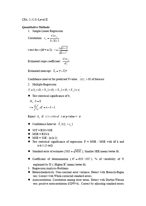
^
H0 : b 0 ˆ t b , df n k 1 sb
Reject h0 if | t | critical t or p-value <
ˆ (t s ) Confidence Interval: b j c bj
Currency appreciates due to: (1) Lower relative income growth rate. (2) Lower relative inflation rate. (3) Higher domestic real interest rate. (4) Improved investment climate. 9. Unanticipated shift to exp. Monetary Policy: Higher income, accelerated inflation, lower real interest rates, leads to currency dept, current acct surplus, and financial acct deficit. 10. Unanticipated shift to exp. Fiscal Policy: currency appr, current acct deficit, & financial account surplus. 11. Purchasing Power Parity: Law of one price: a single, clearly comparable good should have same real price in all countries. Relative PPP: Countries with high inflation rates should see their currencies depreciate.
克鲁格曼 国际经济学第10版 英文答案 国际金融部分krugman_intlecon10_im_14_GE
Chapter 14 (3)Exchange Rates and the Foreign Exchange Market: An Asset ApproachChapter OrganizationExchange Rates and International TransactionsDomestic and Foreign PricesExchange Rates and Relative PricesThe Foreign Exchange MarketThe ActorsBox: Exchange Rates, Auto Prices, and Currency WarsCharacteristics of the MarketSpot Rates and Forward RatesForeign Exchange SwapsFutures and OptionsThe Demand for Foreign Currency AssetsAssets and Asset ReturnsBox: Nondeliverable Forward Exchange Trading in AsiaRisk and LiquidityInterest RatesExchange Rates and Asset ReturnsA Simple RuleReturn, Risk, and Liquidity in the Foreign Exchange MarketEquilibrium in the Foreign Exchange MarketInterest Parity: The Basic Equilibrium ConditionHow Changes in the Current Exchange Rate Affect Expected ReturnsThe Equilibrium Exchange RateInterest Rates, Expectations, and EquilibriumThe Effect of Changing Interest Rates on the Current Exchange RateThe Effect of Changing Expectations on the Current Exchange RateCase Study: What Explains the Carry Trade?SummaryAPPENDIX TO CHAPTER 14 (3): Forward Exchange Rates and Covered Interest Parity© 2015 Pearson Education LimitedChapter OverviewThe purpose of this chapter is to show the importance of the exchange rate in translating foreign prices into domestic values as well as to begin the presentation of exchange rate determination. Central to the treatment of exchange rate determination is the insight that exchange rates are determined in the same way a s other asset prices. The chapter begins by describing how the relative prices of different countries’ goods are affected by exchange rate changes. This discussion illustrates the central importance of exchange rates for cross-border economic linkages. The determination of the level of the exchange rate is modeled in the context of the exchange rate’s role as the relative price of foreign and domestic currencies, using the uncovered interest parity relationship.The euro is used often in examples. Some students may not be familiar with the currency or aware of which countries use it; a brief discussion may be warranted. A full treatment of EMU and the theories surrounding currency unification appears in Chapter 20(9).The description of the foreign exchange market stresses the involvement of large organizations (commercial banks, corporations, nonbank financial institutions, and central banks) and the highly integrated natureof the market. The nature of the foreign exchange market ensures that arbitrage occurs quickly so that common rates are offered worldwide. A comparison of the trading volume in foreign exchange markets to that in other markets is useful to underscore how quickly price arbitrage occurs and equilibrium is restored. Forward foreign exchange trading, foreign exchange futures contracts, and foreign exchange options play an important part in currency market activity. The use of these financial instruments to eliminate short-run exchange rate risk is described.The explanation of exchange rate determination in this chapter emphasizes the modern view that exchange rates move to equilibrate asset markets. The foreign exchange demand and supply curves that introduce exchange rate determination in most undergraduate texts are not found here. Instead, there is a discussion of asset pricing and the determination of expected rates of return on assets denominated in different currencies.Students may already be familiar with the distinction between real and nominal returns. The text demonstrates that nominal returns are sufficient for comparing the attractiveness of different assets. There is a brief description of the role played by risk and liquidity in asset demand, but these considerations are not pursued in this chapter. (The role of risk is taken up again in Chapter 18[7].)Substantial space is devoted to the topic of comparing expected returns on assets denominated in domestic and foreign currency. The text identifies two parts of the expected return on a foreign currency asset (measured in domestic currency terms): the interest payment and the change in the value of the foreign currency relative to the domestic currency over the period in which the asset is held. The expected return on a foreign asset is calculated as a function of the current exchange rate for given expected values of the future exchange rate and the foreign interest rate.The absence of risk and liquidity considerations implies that the expected returns on all assets traded in the foreign exchange market must be equal. It is thus a short step from calculations of expected returns on foreign assets to the interest parity condition. The foreign exchange market is shown to be in equilibrium only when the interest parity condition holds. Thus, for given interest rates and given expectations about future exchange rates, interest parity determines the current equilibrium exchange rate. The interest parity diagram introduced here is instrumental in later chapters in which a more general model is presented. Because a command of this interest parity diagram is an important building block for future work, we recommend drills that employ this diagram.The result that a dollar appreciation makes foreign currency assets more attractive may appear counterintuitive to students—why does a stronger dollar reduce the expected return on dollar assets? The key to explaining this point is that, under the static expectations and constant interest rates assumptions, a dollar appreciation today implies a greater future dollar depreciation; so, an American investor can expect to gain not only theChapter 14Exchange Rates and the Foreign Exchange Market: An Asset Approach 77© 2015 Pearson Education Limitedforeign interest payment but also the extra return due to the dollar’s additional future depreciation. The following diagram illustrates this point. In this diagram, the exchange rate at time t + 1 is expected to be equal to E . If the exchange rate at time t is also E , then expected depreciation is 0. If, however, the exchange rate depreciates at time t to E ', then it must appreciate to reach E at time t + 1. If the exchange rate appreciates today to E ", then it must depreciate to reach E at time t + 1. Thus, under static expectations, a depreciation today implies an expected appreciation and vice versa.Figure 14(3)-1This pedagogical tool can be employed to provide some further intuition behind the interest parityrelationship. Suppose that the domestic and foreign interest rates are equal. Interest parity then requires that the expected depreciation is equal to zero and that the exchange rate today and next period is equal to E . If the domestic interest rate rises, people will want to hold more domestic currency deposits. The resulting increased demand for domestic currency drives up the price of domestic currency, causing the exchange rate to appreciate. How long will this continue? The answer is that the appreciation of the domestic currency continues until the expected depreciation that is a consequence of the domestic currency’s appreciation today just offsets the interest differential.The text presents exercises on the effects of changes in interest rates and of changes in expectations of the future exchange rate. These exercises can help develop students’ intuition. For example, the initial result of a rise in U.S. interest rates is a higher demand for dollar-denominated assets and thus an increase in the price of the dollar. This dollar appreciation is large enough that the subsequent expected dollar depreciation just equalizes the expected return on foreign currency assets (measured in dollar terms) and the higher dollar interest rate.The chapter concludes with a case study looking at a situation in which interest rate parity may not hold: the carry trade. In a carry trade, investors borrow money in low-interest currencies and buy high-interest-rate currencies, often earning profits over long periods of time. However, this transaction carries an element of risk as the high-interest-rate currency may experience an abrupt crash in value. The case study discusses a popular carry trade in which investors borrowed low-interest-rate Japanese yen to purchase high-interest-rate Australian dollars. Investors earned high returns until 2008, when the Australian dollar abruptly crashed, losing 40 percent of its value. This was an especially large loss as the crash occurred amidst a financial crisis in which liquidity was highly valued. Thus, when we factor in this additional risk of the carry trade, interest rate parity may still hold.The Appendix describes the covered interest parity relationship and applies it to explain the determination of forward rates under risk neutrality as well as the high correlation between movements in spot and forward rates.Answers to Textbook Problems1. At an exchange rate of 1.05 $ per euro, a 5 euro bratwurst costs 1.05$/euro ⨯ 5 euros = $5.25. Thus,the bratwurst in Munich is $1.25 more expensive than the hot dog in Boston. The relative price is $5.25/$4 = 1.31. A bratwurst costs 1.31 hot dogs. If the dollar depreciates to 1.25$/euro, the bratwurst now costs 1.25$/euro ⨯ 5 euros = $6.25, for a relative price of $6.25/$4 = 1.56. You have to give up1.56 hot dogs to buy a bratwurst. Hot dogs have become relatively cheaper than bratwurst after thedepreciation of the dollar.2. If it were cheaper to buy Israeli shekels with Swiss francs that were purchased with dollars than todirectly buy shekels with dollars, then people would act upon this arbitrage opportunity. The demand for Swiss francs from people who hold dollars would rise, causing the Swiss franc to rise in value against the dollar. The Swiss franc would appreciate against the dollar until the price of a shekel would be exactly the same whether it was purchased directly with dollars or indirectly through Swiss francs.3. Take for example the exchange rate between the Argentine peso, the US dollar, the euro, and theBritish pound. One dollar is worth 5.3015 pesos, while a euro is worth 7.0089 pesos. To rule out triangular arbitrage, we need to see how many pesos you would get if you first bought euros with your dollars (at an exchange rate of 0.7564 euros per dollar), then used these euros to buy pesos. In other words, we need to compute E D = E EUR/USD × E ARG/EUR = 0.7564× 7.0089 = 5.3015 pesos per dollar. This is almost exactly (with rounding) equal to the direct rate of pesos per dollar.Following the same procedure for the British pound yields a similar result.We need to say that triangular arbitrage is “approximately” ruled out for several reasons. First,rounding error means that there may be some small discrepancies between the direct and indirect exchange rates we calculate. Second, transactions costs on trading currencies will prevent complete arbitrage from occurring. That said, the massive volume of currencies traded make these transactions costs relatively small, leading to “near” perfect arbitrage.4. A depreciation of Chinese yuan makes the import more expensive. Since the demand for oil isinelastic, China needs to import oil from the oil exporting countries. This leads to spending more on oil when the exchange rate falls in value. This can cause the balance of payment to worsen in the short run. Hence, a depreciation of domestic currency may or may not have a favourable impact on the balance of payment in the short run.5. The dollar rates of return are as follows:a. ($250,000 - $200,000)/$200,000 = 0.25.b. ($275 - $255)/$255 = 0.08.c. There are two parts to this return. One is the loss involved due to the appreciation of the dollar;the dollar appreciation is ($1.38 - $1.50)/$1.50 =-0.08. The other part of the return is the interest paid by the London bank on the deposit, 10 percent. (The size of the deposit is immaterial to thecalculation of the rate of return.) In terms of dollars, the realized return on the London depositis thus 2 percent per year.。
Solution_国际财务管理_切奥尔尤恩_课后习题答案_第十四章
CHAPTER 14 INTEREST RATE AND CURRENCY SWAPSSUGGESTED ANSWERS AND SOLUTIONS TO END-OF-CHAPTERQUESTIONS AND PROBLEMSQUESTIONS1. Describe the difference between a swap broker and a swap dealer.Answer: A swap broker arranges a swap between two counterparties for a fee without taking a risk position in the swap. A swap dealer is a market maker of swaps and assumes a risk position in matching opposite sides of a swap and in assuring that each counterparty fulfills its contractual obligation to the other.2. What is the necessary condition for a fixed-for-floating interest rate swap to be possible?Answer: For a fixed-for-floating interest rate swap to be possible it is necessary for a quality spread differential to exist. In general, the default-risk premium of the fixed-rate debt will be larger than the default-risk premium of the floating-rate debt.3. Discuss the basic motivations for a counterparty to enter into a currency swap.Answer: One basic reason for a counterparty to enter into a currency swap is to exploit the comparative advantage of the other in obtaining debt financing at a lower interest rate than could be obtained on its own. A second basic reason is to lock in long-term exchange rates in the repayment of debt service obligations denominated in a foreign currency.4. How does the theory of comparative advantage relate to the currency swap market?Answer: Name recognition is extremely important in the international bond market. Without it, even a creditworthy corporation will find itself paying a higher interest rate for foreign denominated funds than a local borrower of equivalent creditworthiness. Consequently, two firms of equivalent creditworthiness can each exploit their, respective, name recognition by borrowing in their local capital market at a favorable rate and then re-lending at the same rate to the other.5. Discuss the risks confronting an interest rate and currency swap dealer.Answer: An interest rate and currency swap dealer confronts many different types of risk. Interest rate risk refers to the risk of interest rates changing unfavorably before the swap dealer can lay off on an opposing counterparty the unplaced side of a swap with another counterparty. Basis risk refers to the floating rates of two counterparties being pegged to two different indices. In this situation, since the indexes are not perfectly positively correlated, the swap bank may not always receive enough floating rate funds from one counterparty to pass through to satisfy the other side, while still covering its desired spread, or avoiding a loss. Exchange-rate risk refers to the risk the swap bank faces from fluctuating exchange rates during the time it takes the bank to lay off a swap it undertakes on an opposing counterparty before exchange rates change. Additionally, the dealer confronts credit risk from one counterparty defaulting and its having to fulfill the defaulting party’s obligation to the other counterparty. Mismatch risk refers to the difficulty of the dealer finding an exact opposite match for a swap it has agreed to take. Sovereign risk refers to a country imposing exchange restrictions on a currency involved in a swap making it costly, or impossible, for a counterparty to honor its swap obligations to the dealer. In this event, provisions exist for the early termination of a swap, which means a loss of revenue to the swap bank.6. Briefly discuss some variants of the basic interest rate and currency swaps diagramed in the chapter.Answer: Instead of the basic fixed-for-floating interest rate swap, there are also zero-coupon-for-floating rate swaps where the fixed rate payer makes only one zero-coupon payment at maturity on the notional value. There are also floating-for-floating rate swaps where each side is tied to a different floating rate index or a different frequency of the same index. Currency swaps need not be fixed-for-fixed; fixed-for-floating and floating-for-floating rate currency swaps are frequently arranged. Moreover, both currency and interest rate swaps can be amortizing as well as non-amortizing.7. If the cost advantage of interest rate swaps would likely be arbitraged away in competitive markets, what other explanations exist to explain the rapid development of the interest rate swap market?Answer: All types of debt instruments are not always available to all borrowers. Interest rate swaps can assist in market completeness. That is, a borrower may use a swap to get out of one type of financing and to obtain a more desirable type of credit that is more suitable for its asset maturity structure.8. Suppose Morgan Guaranty, Ltd. is quoting swap rates as follows: 7.75 - 8.10 percent annually against six-month dollar LIBOR for dollars and 11.25 - 11.65 percent annually against six-month dollar LIBOR for British pound sterling. At what rates will Morgan Guaranty enter into a $/£ currency swap?Answer: Morgan Guaranty will pay annual fixed-rate dollar payments of 7.75 percent against receiving six-month dollar LIBOR flat, or it will receive fixed-rate annual dollar payments at 8.10 percent against paying six-month dollar LIBOR flat. Morgan Guaranty will make annual fixed-rate £ payments at 11.25 percent against receiving six-month dollar LIBOR flat, or it will receive annual fixed-rate £ payments at 11.65 percent against paying six-month dollar LIBOR flat. Thus, Morgan Guaranty will enter into a currency swap in which it would pay annual fixed-rate dollar payments of 7.75 percent in return for receiving semi-annual fixed-rate £ payments at 11.65 percent, or it will receive annual fixed-rate dollar payments at 8.10 percent against paying annual fixed-rate £ payments at 11.25 percent.9. A U.S. company needs to raise €50,000,000. It plans to raise this money by issuing dollar-denominated bonds and using a currency swap to convert the dollars to euros. The company expects interest rates in both the United States and the euro zone to fall.a. Should the swap be structured with interest paid at a fixed or a floating rate?b. Should the swap be structured with interest received at a fixed or a floating rate?CFA Guideline Answer:a. The U.S. company would pay the interest rate in euros. Because it expects that the interest rate in the euro zone will fall in the future, it should choose a swap with a floating rate on the interest paid in euros to let the interest rate on its debt float down.b. The U.S. company would receive the interest rate in dollars. Because it expects that the interest rate in the United States will fall in the future, it should choose a swap with a fixed rate on the interest received in dollars to prevent the interest rate it receives from going down.*10. Assume a currency swap in which two counterparties of comparable credit risk each borrow at the best rate available, yet the nominal rate of one counterparty is higher than the other. After the initial principal exchange, is the counterparty that is required to make interest payments at the higher nominal rate at a financial disadvantage to the other in the swap agreement? Explain your thinking.Answer: Superficially, it may appear that the counterparty paying the higher nominal rate is at a disadvantage since it has borrowed at a lower rate. However, if the forward rate is an unbiased predictor of the expected spot rate and if IRP holds, then the currency with the higher nominal rate is expected to depreciate versus the other. In this case, the counterparty making the interest payments at the higher nominal rate is in effect making interest payments at the lower interest rate because the payment currency is depreciating in value versus the borrowing currency.PROBLEMS1. Alpha and Beta Companies can borrow for a five-year term at the following rates:Alpha BetaMoody’s credit rating Aa BaaFixed-rate borrowing cost 10.5% 12.0%Floating-rate borrowing cost LIBOR LIBOR + 1%a. Calculate the quality spread differential (QSD).b. Develop an interest rate swap in which both Alpha and Beta have an equal cost savings in their borrowing costs. Assume Alpha desires floating-rate debt and Beta desires fixed-rate debt. No swap bank is involved in this transaction.Solution:a. The QSD = (12.0% - 10.5%) minus (LIBOR + 1% - LIBOR) = .5%.b. Alpha needs to issue fixed-rate debt at 10.5% and Beta needs to issue floating rate-debt at LIBOR + 1%. Alpha needs to pay LIBOR to Beta. Beta needs to pay 10.75% to Alpha. If this is done, Alpha’s floating-rate all-in-cost is: 10.5% + LIBOR - 10.75% = LIBOR - .25%, a .25% savings over issuing floating-rate debt on its own. Beta’s fixed-rate all-in-cost is: LIBOR+ 1% + 10.75% - LIBOR = 11.75%, a .25% savings over issuing fixed-rate debt.2. Do problem 1 over again, this time assuming more realistically that a swap bank is involved as an intermediary. Assume the swap bank is quoting five-year dollar interest rate swaps at 10.7% - 10.8% against LIBOR flat.Solution: Alpha will issue fixed-rate debt at 10.5% and Beta will issue floating rate-debt at LIBOR + 1%. Alpha will receive 10.7% from the swap bank and pay it LIBOR. Beta will pay 10.8% to the swap bank and receive from it LIBOR. If this is done, Alpha’s floating-rate all-in-cost is: 10.5% + LIBOR - 10.7% = LIBOR - .20%, a .20% savings over issuing floating-rate debt on its own. Beta’s fixed-rate all-in-cost is: LIBOR+ 1% + 10.8% - LIBOR = 11.8%, a .20% savings over issuing fixed-rate debt.3. Company A is a AAA-rated firm desiring to issue five-year FRNs. It finds that it can issue FRNs at six-month LIBOR + .125 percent or at three-month LIBOR + .125 percent. Given its asset structure, three-month LIBOR is the preferred index. Company B is an A-rated firm that also desires to issue five-year FRNs. It finds it can issue at six-month LIBOR + 1.0 percent or at three-month LIBOR + .625 percent. Given its asset structure, six-month LIBOR is the preferred index. Assume a notional principal of $15,000,000. Determine the QSD and set up a floating-for-floating rate swap where the swap bank receives .125 percent and the two counterparties share the remaining savings equally.Solution: The quality spread differential is [(Six-month LIBOR + 1.0 percent) minus (Six-month LIBOR + .125 percent) =] .875 percent minus [(Three-month LIBOR + .625 percent) minus (Three-month LIBOR + .125 percent) =] .50 percent, which equals .375 percent. If the swap bank receives .125 percent, each counterparty is to save .125 percent. To affect the swap, Company A would issue FRNs indexed to six-month LIBOR and Company B would issue FRNs indexed three-month LIBOR. Company B might make semi-annual payments of six-month LIBOR + .125 percent to the swap bank, which would pass all of it through to Company A. Company A, in turn, might make quarterly payments of three-month LIBOR to the swap bank, which would pass through three-month LIBOR - .125 percent to Company B. On an annualized basis, Company B will remit to the swap bank six-month LIBOR + .125 percent and pay three-month LIBOR + .625 percent on its FRNs. It will receive three-month LIBOR - .125 percent from the swap bank. This arrangement results in an all-in cost of six-month LIBOR + .825 percent, which is a rate .125 percent below the FRNs indexed to six-month LIBOR + 1.0 percent Company B could issue on its own. Company A will remit three-month LIBOR to the swap bank and pay six-month LIBOR + .125 percent on its FRNs. It will receive six-month LIBOR + .125 percent from the swap bank. This arrangement results in an all-in cost of three-month LIBOR for Company A, which is .125 percent less than the FRNs indexed to three-month LIBOR + .125 percent it could issue on its own. The arrangements with the two counterparties net the swap bank .125 percent per annum, received quarterly.*4. A corporation enters into a five-year interest rate swap with a swap bank in which it agrees to pay the swap bank a fixed rate of 9.75 percent annually on a notional amount of €15,000,000 and receive LIBOR. As of the second reset date, determine the price of the swap from the corporation’s viewpoint assuming that the fixed-rate side of the swap has increased to 10.25 percent.Solution: On the reset date, the present value of the future floating-rate payments the corporation will receive from the swap bank based on the notional value will be €15,000,000. The present value of a hypothetical bond issue of €15,000,000 with three remaining 9.75 percent coupon payments at the newfixed-rate of 10.25 percent is €14,814,304. This sum represents the present value of the remaining payments the swap bank will receive from the corporation. Thus, the swap bank should be willing to buy and the corporation should be willing to sell the swap for €15,000,000 - €14,814,304 = €185,696.5. Karla Ferris, a fixed income manager at Mangus Capital Management, expects the current positively sloped U.S. Treasury yield curve to shift parallel upward.Ferris owns two $1,000,000 corporate bonds maturing on June 15, 1999, one with a variable rate based on 6-month U.S. dollar LIBOR and one with a fixed rate. Both yield 50 basis points over comparable U.S. Treasury market rates, have very similar credit quality, and pay interest semi-annually.Ferris wished to execute a swap to take advantage of her expectation of a yield curve shift and believes that any difference in credit spread between LIBOR and U.S. Treasury market rates will remain constant.a. Describe a six-month U.S. dollar LIBOR-based swap that would allow Ferris to take advantage of her expectation. Discuss, assuming Ferris’ expectation is correct, the change in the swap’s value and how that change would affect the value of her portfolio. [No calculations required to answer part a.] Instead of the swap described in part a, Ferris would use the following alternative derivative strategy to achieve the same result.b. Explain, assuming Ferris’ expectation is correct, how the following strategy achieves the same result in response to the yield curve shift. [No calculations required to answer part b.]Date Nominal Eurodollar Futures Contract ValueSettlement12-15-97 $1,000,00003-15-98 1,000,00006-15-98 1,000,00009-15-98 1,000,00012-15-98 1,000,00003-15-99 1,000,000c. Discuss one reason why these two derivative strategies provide the same result.CFA Guideline Answera.The Swap Value and its Effect on Ferris’ PortfolioBecause Karla Ferris believes interest rates will rise, she will want to swap her $1,000,000 fixed-rate corporate bond interest to receive six-month U.S. dollar LIBOR. She will continue to hold her variable-rate six-month U.S. dollar LIBOR rate bond because its payments will increase as interest rates rise. Because the credit risk between the U.S. dollar LIBOR and the U.S. Treasury market is expected to remain constant, Ferris can use the U.S. dollar LIBOR market to take advantage of her interest rate expectation without affecting her credit risk exposure.To execute this swap, she would enter into a two-year term, semi-annual settle, $1,000,000 nominal principal, pay fixed-receive floating U.S. dollar LIBOR swap. If rates rise, the swap’s mark-to-market value will increase because the U.S. dollar LIBOR Ferris receives will be higher than the LIBOR rates from which the swap was priced. If Ferris were to enter into the same swap after interest rates rise, she would pay a higher fixed rate to receive LIBOR rates. This higher fixed rate would be calculated as the present value of now higher forward LIBOR rates. Because Ferris would be paying a stated fixed rate that is lower than this new higher-present-value fixed rate, she could sell her swap at a premium. This premium is called the “replacement cost” value of the swap.b. Eurodollar Futures StrategyThe appropriate futures hedge is to short a combination of Eurodollar futures contracts with different settlement dates to match the coupon payments and principal. This futures hedge accomplishes the same objective as the pay fixed-receive floating swap described in Part a. By discussing how the yield-curve shift affects the value of the futures hedge, the candidate can show an understanding of how Eurodollar futures contracts can be used instead of a pay fixed-receive floating swap.If rates rise, the mark-to-market values of the Eurodollar contracts decrease; their yields must increase to equal the new higher forward and spot LIBOR rates. Because Ferris must short or sell the Eurodollar contracts to duplicate the pay fixed-receive variable swap in Part a, she gains as the Eurodollar futures contracts decline in value and the futures hedge increases in value. As the contracts expire, or if Ferris sells the remaining contracts prior to maturity, she will recognize a gain that increases her return. With higher interest rates, the value of the fixed-rate bond will decrease. If the hedge ratios are appropriate, the value of the portfolio, however, will remain unchanged because of the increased value of the hedge, which offsets the fixed-rate bond’s decrease.c. Why the Derivative Strategies Achieve the Same ResultArbitrage market forces make these two strategies provide the same result to Ferris. The two strategies are different mechanisms for different market participants to hedge against increasing rates. Some money managers prefer swaps; others, Eurodollar futures contracts. Each institutional marketparticipant has different preferences and choices in hedging interest rate risk. The key is that market makers moving into and out of these two markets ensure that the markets are similarly priced and provide similar returns. As an example of such an arbitrage, consider what would happen if forward market LIBOR rates were lower than swap market LIBOR rates. An arbitrageur would, under such circumstances, sell the futures/forwards contracts and enter into a received fixed-pay variable swap. This arbitrageur could now receive the higher fixed rate of the swap market and pay the lower fixed rate of the futures market. He or she would pocket the differences between the two rates (without risk and without having to make any [net] investment.) This arbitrage could not last.As more and more market makers sold Eurodollar futures contracts, the selling pressure would cause their prices to fall and yields to rise, which would cause the present value cost of selling the Eurodollar contracts also to increase. Similarly, as more and more market makers offer to receive fixed rates in the swap market, market makers would have to lower their fixed rates to attract customers so they could lock in the lower hedge cost in the Eurodollar futures market. Thus, Eurodollar forward contract yields would rise and/or swap market receive-fixed rates would fall until the two rates converge. At this point, the arbitrage opportunity would no longer exist and the swap and forwards/futures markets would be in equilibrium.6. Rone Company asks Paula Scott, a treasury analyst, to recommend a flexible way to manage the company’s financial risks.Two years ago, Rone issued a $25 million (U.S.$), five-year floating rate note (FRN). The FRN pays an annual coupon equal to one-year LIBOR plus 75 basis points. The FRN is non-callable and will be repaid at par at maturity.Scott expects interest rates to increase and she recognizes that Rone could protect itself against the increase by using a pay-fixed swap. However, Rone’s Board of Directors prohibits both short sales of securities and swap transactions. Scott decides to replicate a pay-fixed swap using a combination of capital market instruments.a. Identify the instruments needed by Scott to replicate a pay-fixed swap and describe the required transactions.b. Explain how the transactions in Part a are equivalent to using a pay-fixed swap.CFA Guideline Answera. The instruments needed by Scott are a fixed-coupon bond and a floating rate note (FRN).The transactions required are to:· issue a fixed-coupon bond with a maturity of three years and a notional amount of $25 million, and· buy a $25 million FRN of the same maturity that pays one-year LIBOR plus 75 bps.b. At the outset, Rone will issue the bond and buy the FRN, resulting in a zero net cash flow at initiation. At the end of the third year, Rone will repay the fixed-coupon bond and will be repaid the FRN, resulting in a zero net cash flow at maturity. The net cash flow associated with each of the three annual coupon payments will be the difference between the inflow (to Rone) on the FRN and the outflow (to Rone) on the bond. Movements in interest rates during the three-year period will determine whether the net cash flow associated with the coupons is positive or negative to Rone. Thus, the bond transactions are financially equivalent to a plain vanilla pay-fixed interest rate swap.7. A company based in the United Kingdom has an Italian subsidiary. The subsidiary generates €25,000,000 a year, received in equivalent semiannual installments of €12,500,000. The British company wishes to convert the euro cash flows to pounds twice a year. It plans to engage in a currency swap in order to lock in the exchange rate at which it can convert the euros to pounds. The current exchange rate is €1.5/£. The fixed rate on a plain vaninilla currency swap in pounds is 7.5 percent per year, and the fixed rate on a plain vanilla currency swap in euros is 6.5 percent per year.a. Determine the notional principals in euros and pounds for a swap with semiannual payments that will help achieve the objective.b. Determine the semiannual cash flows from this swap.CFA Guideline Answera. The semiannual cash flow must be converted into pounds is €25,000,000/2 = €12,500,000. In order to create a swap to convert €12,500,000, the equivalent notional principals are · Euro notional principal = €12,500,000/(0.065/2) = €384,615,385· Pound notional principal = €384,615,385/€1.5/£ = £256,410,257b. The cash flows from the swap will now be· Company makes swap payment = €384,615,385(0.065/2) = €12,500,000· Company receives swap payment = £256,410,257(0.075/2) = £9,615,385The company has effectively converted euro cash receipts to pounds.8. Ashton Bishop is the debt manager for World Telephone, which needs €3.33 billion Euro financing for its operations. Bishop is considering the choice between issuance of debt denominated in: ∙ Euros (€), or∙ U.S. dollars, accompanied by a combined interest rate and currency swap.a. Explain one risk World would assume by entering into the combined interest rate and currency swap.Bishop believes that issuing the U.S.-dollar debt and entering into the swap can lower World’s cost of debt by 45 basis points. Immediately after selling the debt issue, World would swap the U.S. dollar payments for Euro payments throughout the maturity of the debt. She assumes a constant currency exchange rate throughout the tenor of the swap.Exhibit 1 gives details for the two alternative debt issues. Exhibit 2 provides current information about spot currency exchange rates and the 3-year tenor Euro/U.S. Dollar currency and interest rate swap.Exhibit 1World Telephone Debt DetailsCharacteristic Euro Currency Debt U.S. Dollar Currency DebtPar value €3.33 billion $3 billionTerm to maturity 3 years 3 yearsFixed interest rate 6.25% 7.75%Interest payment Annual AnnualExhibit 2Currency Exchange Rate and Swap InformationSpot currency exchange rate $0.90 per Euro ($0.90/€1.00)3-year tenor Euro/U.S. Dollarfixed interest rates 5.80% Euro/7.30% U.S. Dollarb. Show the notional principal and interest payment cash flows of the combined interest rate and currency swap.Note: Your response should show both the correct currency ($ or €) and amount for each cash flow. Answer problem b in the template provided.Template for problem bc. State whether or not World would reduce its borrowing cost by issuing the debt denominated in U.S. dollars, accompanied by the combined interest rate and currency swap. Justify your response with one reason.CFA Guideline Answera. World would assume both counterparty risk and currency risk. Counterparty risk is the risk that Bishop’s counterparty will default on payment of principal or interest cash flows in the swap.Currency risk is the currency exposure risk associated with all cash flows. If the US$ appreciates (Euro depreciates), there would be a loss on funding of the coupon payments; however, if the US$ depreciates, then the dollars will be worth less at the swap’s maturity.b.0 YearYear32 Year1 YearWorld paysNotional$3 billion €3.33 billion PrincipalInterest payment €193.14 million1€193.14 million €193.14 million World receives$3.33 billion €3 billion NotionalPrincipalInterest payment $219 million2$219 million $219 million1 € 193.14 million = € 3.33 billion x 5.8%2 $219 million = $3 billion x 7.3%c. World would not reduce its borrowing cost, because what Bishop saves in the Euro market, she loses in the dollar market. The interest rate on the Euro pay side of her swap is 5.80 percent, lower than the 6.25 percent she would pay on her Euro debt issue, an interest savings of 45 bps. But Bishop is only receiving 7.30 percent in U.S. dollars to pay on her 7.75 percent U.S. debt interest payment, an interest shortfall of 45 bps. Given a constant currency exchange rate, this 45 bps shortfall exactly offsets the savings from paying 5.80 percent versus the 6.25 percent. Thus there is no interest cost savings by sellingthe U.S. dollar debt issue and entering into the swap arrangement.MINI CASE: THE CENTRALIA CORPORATION’S CURRENCY SWAPThe Centralia Corporation is a U.S. manufacturer of small kitchen electrical appliances. It has decided to construct a wholly owned manufacturing facility in Zaragoza, Spain, to manufacture microwave ovens for sale in the European Union. The plant is expected to cost €5,500,000, and to take about one year to complete. The plant is to be financed over its economic life of eight years. The borrowing capacity created by this capital expenditure is $2,900,000; the remainder of the plant will be equity financed. Centralia is not well known in the Spanish or international bond market; consequently, it would have to pay 7 percent per annum to borrow euros, whereas the normal borrowing rate in the euro zone for well-known firms of equivalent risk is 6 percent. Alternatively, Centralia can borrow dollars in the U.S. at a rate of 8 percent.Study Questions1. Suppose a Spanish MNC has a mirror-image situation and needs $2,900,000 to finance a capital expenditure of one of its U.S. subsidiaries. It finds that it must pay a 9 percent fixed rate in the United States for dollars, whereas it can borrow euros at 6 percent. The exchange rate has been forecast to be $1.33/€1.00 in one year. Set up a currency swap that will benefit each counterparty.*2. Suppose that one year after the inception of the currency swap between Centralia and the Spanish MNC, the U.S. dollar fixed-rate has fallen from 8 to 6 percent and the euro zone fixed-rate for euros has fallen from 6 to 5.50 percent. In both dollars and euros, determine the market value of the swap if the exchange rate is $1.3343/€1.00.Suggested Solution to The Centralia Corporation’s Currency Swap1. The Spanish MNC should issue €2,180,500 of 6 percent fixed-rate debt and Centralia should issue $2,900,000 of fixed-rate 8 percent debt, since each counterparty has a relative comparative advantage in their home market. They will exchange principal sums in one year. The contractual exchange rate for the initial exchange is $2,900,000/€2,180,500, or $1.33/€1.00. Annually the counterparties will swap debt service: the Spanish MNC will pay Centralia $232,000 (= $2,900,000 x .08) and Centralia will pay the Spanish MNC €130,830 (= €2,180,500 x .06). The contractual exchange rate of the first seven annual debt service exchanges is $232,000/€130,830, or $1.7733/€1.00. At maturity, Centralia and the Spanish MNC will re-exchange the principal sums and the final debt service payments. The contractual exchange rate of the final currency exchange is $3,132,000/€2,311,330 = ($2,900,000 + $232,000)/(€2,180,500 + €130,830), or $1.3551/€1.00.*2. The market value of the dollar debt is the present value of a seven-year annuity of $232,000 and a lump sum of $2,900,000 discounted at 6 percent. This present value is $3,223,778. Similarly, the market value of the euro debt is the present value of a seven-year annuity of €130,830 and a lump sum of €2,180,500 discounted at 5.50 percent. This present value is €2,242,459. The dollar value of the swap is $3,223,778 - €2,242,459 x 1.3343 = $231,665. The euro value of the swap is €2,242,459 - $3,223,778/1.3343 = -€173,623.。
Chapter 13 Exchange Rates and the Foreign Exchan
Example
Party A: Euro1 Party B:Euro 1.2420/25 Party A:20 Done
My Euro TO A Frankfurt A/C Party B:Agree
CFM at 2.2420 We Buy USD 1 MIO AG Euro Val Sep 10 USD To B NY TKS For Calling N Deal BIBI
corporations corporations corporations
ns
13-2-3 Characteristics of the Market
Immense trade volume Concentrated Rapid growth Integrated and highly efficient The US dollar involved mostly
Running broker
Actors
central banks
Central bankss
brokers
brokers
Commercialbanks Commercialbanks Commercialbanks Commercialbanks
B ro k e rs Nonbankfinancialinstitutions Nonbankfinancialinstitutions Nonbankfinancialinstitutions Nonbankfinancialinstitutions
US$ Quotation:The price of dollars in terms of one country’s currency.
- 1、下载文档前请自行甄别文档内容的完整性,平台不提供额外的编辑、内容补充、找答案等附加服务。
- 2、"仅部分预览"的文档,不可在线预览部分如存在完整性等问题,可反馈申请退款(可完整预览的文档不适用该条件!)。
- 3、如文档侵犯您的权益,请联系客服反馈,我们会尽快为您处理(人工客服工作时间:9:00-18:30)。
ASSET MARKETS, EXCHANGE RATES AND THE BALANCE OF PAYMENTS JACOB A. FRENKEL and MICHAEL L. MUSSA*University of Chicago and national Bureau of Economic ResearchContents1. Introduction2. The Mundell-Fleming model3. The dynamics of balance of payments adjustment under fixed exchange rates3.1 Adjustment in a small open economy without capital mobility3.2 Extensions of the simple model4. Flexible exchange rates4.1 The monetary model of exchange rate determination4.2 Exchange rates as asset prices4.3 Balance of payments equilibrium and the real exchange rate4.4 Exchange rates and money in the general model of exchange rate determination4.5 Empirical issues in exchange rate analysisReferences*We are grateful to Stanley Black, William Branson and peter Kenen for helpful comments on an earlier draft of this paper. The research reported here is part of the NBER’s research program in International Studies and Economic Fluctuations. Any opinions expressed are those of the authors and not necessarily those of the NBER. Handbook of International Economics, vo l.ІІ, edited by R.W. Jones and P.B. KenenElsevier Science Publishers B.V., 19851. IntroductionThis chapter reviews developments in international monetary economics from the late 1960s through the early 1980s. Since the world remained on a system of fixed exchange rates until 1973, most of the research in the earlier part of this period focused on monetary relationships and macroeconomic behavior of open economies under a system of fixed exchange rates. An issue of central importance in this research, including the extensive literature on the "monetary approach to the balance of payments", was the economic determinants of the behavior of the balance of payments, especially, the theoretical elaboration and empirical investigation of the dynamic mechanism of balance of payments adjustment. With the shift to a system of floating exchange rates among major currencies in 1973, there was a corresponding shift of research interests away from primary focus on the balance of payments and to principal concern with the economic determinants of the behavior of exchange rates. The unifying theme in much of this research was the "asset market approach to exchange rates" which emphasizes conditions for equilibrium in the markets for stocks of assets, especially national monies, as the proximate determinant of the behavior of exchange rates.Three general features of the research surveyed in this chapter distinguish it, in general emphasis and broad outline, from the earlier work on international monetary economics surveyed in Chapter 13 of this Handbook by Kenen. First, in the policy approach to open economy macroeconomics developed most extensively by Meade (1951), and extended by the important work of Mundell (1968c) and Fleming (1962), it is usually assumed that the level of national income is controlled by government policy, and that maintenance of full employment (or internal balance) is the paramount objective of economic policy. In this approach, the balance of payments is a "problem" because maintenance of balance of payments equilibrium (or external balance) constrains the use of macroeconomic policy for purposes of maintaining full employment. This problem can be satisfactorily resolved provided that governments have an adequate number of independent and effective policy instruments. More recent research on macroeconomics, for both closed and open economies, expresses far less confidence in the ability of governments to systematically affect levels of national income and consistently maintain full employment through policy manipulation. This view is reflected in the more recent research on international monetary economics where the balance of payments and the exchange rate are regarded as important in their own fight, rather than as subsidiary concerns of policy management.Second, in much of the earlier work on international monetary economics, policy actions and economic disturbances were assumed to have essentially permanent effects on payments flows. It was recognized, of course, that the losses of foreign exchange reserves associated with official settlements deficits would imply a declining domestic money supply, unless the monetary effects of the reserve loss were sterilized by domestic credit expansion. It was also recognized that reserve losses sterilized by domestic credit expansion could not go on forever because a government would ultimately run out of reserves. However, relatively little attention was paid to the dynamic process that would operate if reserve losses (or gains) were allowed to affect the money supply, or to the long run equilibrium that would be established if this process were allowed to operate, or to the longer run consequences of changes in supplies of securities necessarily associated with policies of sterilizing reserve losses and gains. In contrast, in the research surveyed here, the dynamic interaction among asset stocks and payments flows is at the center stage of the analysis.Third, in earlier work on exchange rate theory, the condition for equilibrium in the flow market for foreign exchange transactions (exports, imports, and capital flows) was usually regarded as the proximate determinant of the exchange rate. In some analyses, expectations of future exchange rates had an important influence on currentexchange rates by affecting speculative capital flows. But, even in these analyses, expectations of future exchange rates were usually determined exogenously or by some ad hoc expectations mechanism. Recent research on the theory of exchange rates, in contrast, has focused more on the conditions for asset market equilibrium as the proximate determinant of equilibrium exchange rates, and has usually regarded expectations of future exchange rates as a critical factor affecting the conditions for equilibrium in the relevant asset markets. Moreover, by adopting the assumption of "rational expectations," many recent models of exchange rate behavior have allowed for endogenous determination of expectations of future exchange rates in a manner consistent with the structure of the economic system, and have thereby permitted explicit analysis of the role of information in forming and revising expectations critical to explaining the behavior of exchange rates.Differences between the research surveyed in this chapter and earlier approaches to balance of payments analysis and exchange rate theory should not, however, be overemphasized. The theoretical models applied to balance of payments analysis in the late 1960s and early 1970s incorporate the same basic elements as earlier such models and, correspondingly, share many of the same properties and implications. This essential unity is emphasized in this survey by beginning our discussion, in Section 2, with a review of the operation of the monetary mechanism of balance of payments adjustment in the context of the Meade-Mundell-Fleming model of open economy macroeconomics. We then turn in Section 3 to the more modern analysis of the dynamics of balance of payments adjustment under fixed exchange rates beginning with a simple exposition of the key elements of the monetary mechanism of balance of payments adjustment. The simple model is then extended to incorporate sluggish wage and output adjustments, endogenous monetary policy and sterilization operations, multiplicity of tradable and non-tradable goods, the case of large countries with endogenously determined terms of trade and, finally, capital mobility and portfolio balance.Section 4 deals with the theory of flexible exchange rates. The evolution of the international monetary system from a regime of pegged exchange rates into a regime of flexible rates resulted in a renewed interest in the theory of exchange rate determination. Analogously to the characteristics of the modern theory of the balance of payments under fixed exchange rates, the modern theory of exchange rate determination has shifted the emphasis from the circular flow approach (that gained popularity with the Keynesian revolution) to considerations of portfolio choice and stock equilibrium. A consequence of this shift has been the development of the asset-market approach to the determination of exchange rates. Models which belong to the general category of the asset-market approach differ in their emphasis on the role of money and the other assets but they all highlight the roles of expectations and of stock equilibrium.Our exposition of exchange-rate theory starts with a simple exposition of the monetary approach to exchange-rate determination. In this context we highlight the roles of purchasing power parities, non-traded goods, the real exchange rate, currency substitution, as well as the interaction between real and monetary factors which determine the equilibrium exchange rate. We then present a more general framework that views the question of exchange-rate determination as part of the general theory of the determination of asset prices. The broader framework highlights the unique role of expectations. The general framework is then used to characterize the interaction between the balance of payments and the equilibrium real exchange rate. This model shows that the current exchange rate depends on the entire expected future time paths of the relevant exogenous variables. The section concludes with a brief discussion of some empirical issues for exchange-rate analysis.2. The Mundell-Fleming modeli The key development in the area of balance of payments analysis in the late 1960sand early 1970s was the theoretical elaboration and empirical investigation of the dynamic mechanism of balance of payments adjustment. The essential idea of this dynamic mechanism, which dates back to Hume's discussion of the price-specie-flow mechanism, is that changes in asset stocks (especially the money supply) associated with payments imbalances alter the instantaneous equilibrium position of the economy over time and ultimately drive it to a long-run equilibrium at which the payments imbalance is eliminated. In much of the literature on balance of payments theory and open economy macroeconomics of the 1950s and 1960s,this dynamic mechanism of balance of payments adjustment was either ignored or suppressed by assuming that the domestic monetary authority sterilized the monetary effects of foreign exchange reserve gains and loses. However, at least in Mundell's (1961) description of the international disequilibrium system, this dynamic mechanism was explicitly introduced into the standard model that represented the main line of development in this earlier literature.As illustrated in Figure 2.1, Mundell's analysis is based on the open economy extension of the IS-LM model, frequently referred to as the Mundell-Fleming model. In this diagram, the positively sloped LM curves show combinations of national income, Y , and the domestic nominal interest rate, i, for which the real demand for domestic money, L (Y, i ) (where ∂L/∂Y>O and ∂L/∂i<O ), is equal to the real supply, M/P . The different LM curves are all drawn for the same, parametrically determined domestic price level, P, but for different levels of the domestic nominal money supply, M, with lower LM curves corresponding to larger domestic nominal money supplies. The negatively sloped IS curve indicates the combinations of Y and i for which the demand for national product is equal to national income. The demand for national product is the sum of domestic demand forFigure 2.1. Monetary policy and devaluation in the Mundell-Fleming model with limited capital mobilityproduct, D(Y, i; τ) (where ∂D/∂Y > O, ∂D/∂i < O, and ∂D/∂τ< 0), plus foreign demand for domestic product, I*(τ) (where ∂I*/∂τ< 0); τ = P/S ·P* is the terms of trade between domestic goods and foreign goods, where P* denotes the foreign price of foreign goods and S denotes the exchange rate which is defined as the price of foreign exchange in terms of domestic currency. Alternatively, the demand for national product is the sum of total domestic expenditure, E (Y , i) (where 1 >∂E/∂Y>∂D/∂Y> 0 and ∂E/∂i < o) plus the trade balancesurplus In that alternative formulation, total domes- tic expenditure includes expenditure on imports, I (Y, i; τ) = E (Y, i) - D (Y, i; τ), and, using this expression, the trade balance surplus is, T (Y, i; τ) = I*(τ) - I( Y, i; τ), where ∂T/∂Y < 0, ∂T/∂i > 0, ∂T/∂τ < 0. The positively sloped FF curve shows combinations of Y and i for which the trade balance is zero.1The terms of trade,τ, is a parameter affecting the positions of the IS and FF curves.At any moment of time, the instantaneous equilibrium position of the economy is determined by the intersection of the IS curve and the LM curve drawn for the current money supply. In particular, when the money supply is M0and the terms of trade is τ0, the instantaneous equilibrium point is at A0in Figure 2.1. At this instantaneous equilibrium, the trade balance is in surplus, as indicated by the fact that A0 is above and to the left of the FF curve. Since the present analysis assumes an absence of private capital flows, it follows that for the government to maintain a fixed exchange rate, it must purchase foreign exchange reserves at a rate equal to the trade surplus at A0. If the government does not sterilize the monetary effects of this reserve accumulation, the domestic nominal money supply will grow at a rate equal to the rate of accumulation of foreign exchange reserves, valued in domestic money. Growth of M gradually shifts the LM curve in Figure 2.1 downward and to the right, moving the instantaneous equilibrium point along the IS curve away from A0and toward the point A determined by the intersection of the IS and FF curves. When the instantaneous equilibrium point (and the LM curve) reach A, the trade balance is zero, accumulation of foreign exchange reserves ceases, and economy is in long-run equilibrium. The dynamic mechanism which drives the economy from A0(or any other initial instantaneous equilibrium position) to long-run equilibrium at A is the monetary mechanism of balance of payments adjustment. The total accumulation of foreign exchange reserve (the cumulative official settlements surplus) associated with the movement from A0 to A, valued in domestic money, is determined by the difference between the initial nominal money supply, M0, and the long run equilibrium level of the money supply, M=P0·L(Y, i), where Y and i are the long-run equilibrium levels of Y and i that are associated with the long-run equilibrium point A.Starting at the instantaneous equilibrium A0, if the money supply were increased by a domestic credit expansion to the extent of the difference between M0 and M, the result would be an immediate shift of the LM curve to its long-run equilibrium position and an immediate jump of national income and the domestic interest rate to their respective long-run equilibrium values. As a consequence of this domestic credit expansion, therefore, the government would forgo the increase in foreign exchange reserves that would otherwise occur as a consequence of the natural adjustment process of the economy in moving from A0 to A, but would gain a more immediate increase in the level of national income. Alternatively, if the government expanded domestic credit starting from a situation of long-run equilibrium, it would temporarily shift the LM curve downward and to the right, creating an instantaneous equilibrium at a point like A1 corresponding to the higher quantity of money, M1. At A1, there would be a balance of payments deficit, and the gradual adjustment of the domestic money Supply implied by losses of foreign exchange reserves would ultimately drive the instantaneous equilibrium point back to A. In the long run, therefore, the increase in the domestic credit component of the money supply would be fully offset by an equal loss of foreign exchange reserves, and the stimulative effect of the domestic credit expansion on national income would only be temporary. If the government attempted to maintain national income at a level above its long-run equilibrium level by sterilizing foreign exchange reserve losses through offsetting1 ln Figure 2.1 the FFcurve is drawn steeper than the LM curve in order to emphasize that at thisstage of the analysis we rule out private capital flows. This assumption is modified below.i 0Y FF domestic credit expansions, it could do so for a while, but ultimately it would run out of reserves.A devaluation from an initial equilibrium at A increases S and reduces τ from τ0 to τ1 (since in this analysis P and P* are assumed to be given) shifting both the IS and FF curves to the right to IS (τ1) and FF (τ1), respectively. The new long-run equilibrium is at A ’, with a higher long run equilibrium level of national income, Y ', and a lower long-run equilibrium level of the domestic interest rate, i’ .2 If at the time of this devaluation, the money supply was at the long-run equilibrium level appropriate for the old exchange rate, the impact effect of the devaluation will be to move the instantaneous equilibrium point up along the LM curve passing through A to the intersection between this LM curve and the new IS curve as illustrated by point A 0’. The impact effect of devaluation, therefore, is to increase domestic income and the domestic interest rate and to create a balance of payments surplus. These impact effects of devaluation, however, are not the permanent, long-run effects of devaluation. Increases in the money supply resulting from payments surpluses that are the short-run consequence of the devaluation drive the economy to its new long-run equilibrium A ’ at which domestic income is higher and the domestic interest rate is lower than A 0 and at which the (flow) balance of payments surplus initially created by the devaluation is eliminated. With respect to the balance of payments, therefore, the long-run effect of devaluation is a permanent, cumulative change in the level of reserves equal to increase in the long run equilibrium size of the nominal money supply from M = L (Y , i) to M 1=M '= L (Y ’, i’), but not a permanent surplus in the flow magnitude of the balance of payments.When privately held financial assets are internationally mobile, this analysis of the balance of payments adjustment mechanism needs to be modified to take account of the effects of capital movements on reserve holdings and national money supplies. Specifically, with perfect capital mobility, the FF curve indicating balance of payments equilibrium becomes a horizontal line at the level of the world interest rate, i*, as indicated in Figure2.2. In this situation an instantaneous equilibrium at a point like A 0, determined by the IS curve and the LM curveFigure 2.2. The Mundell-Fleming model with perfect capital mobility.for a domestic money supply of M 0, is not sustainable as an instantaneous equilibrium because a domestic interest rate i 0 that is above the world interest rate i* would induce a huge capital inflow. Domestic residents would sell securities to foreigners in order to increase their money balances to the level consistent with i=i*. The increase in reserves implied by this capital inflow causes the LM curve to jump until it passes through the 2 This result follows from the fact that the horizontal shift of the FF curve is larger than the corresponding shift of the IS curve since ∂E/∂Y < 1. Both curves shift to the right since income must rise to offset the impact of the fall in T on demand.long-run equilibrium point A determined by the intersect/on of the IS curve with the FF curve. Thus, with perfect capital mobility, the balance of payments adjustment process is not a gradual process in which money supply gradually adjusts to reserve gains and losses associated with trade imbalances, but rather an instantaneous adjustment process in which the level of reserves adjusts immediately in response to international capital movements.The essential elements in this analysis of the mechanism of balance of payments adjustment, including the analysis of the cumulative effects on the balance of payments of changes in domestic credit or the exchange rate and of the consequences of international capital mobility arc also central in the literature on balance of payments theory that developed during the late 1960s and early 1970s. In this literature, however, less reliance is placed on the Keynesian assumptions of rigid domestic prices and demand determined output levels as the relevant assumptions for balance of payments analysis, and more attention is devoted to explicit modelling of the dynamics of the balance of payments adjustment process. The analysis in Section 3 focuses on these issues.3. The dynamics of balance of payments adjustment under fixed exchange rates3.1. Adjustment in a small open economy without capital mobility.To illustrate the monetary mechanism of balance of payments adjustment consider first a small open economy facing given world relative prices of all (tradable) goods produced and consumed by domestic residents. Using the Hicksian aggregation principle, domestic real income (equal to domestic output), Y, and domes-tic real expenditure, E, are measured in common units of a composite tradable good. Domestic real income is constant at the level determined by full employment of domestic resources. Domestic real expenditure depends on domestic real income, the domestic real interest rate, r, and the real value of privately held domestic assets, A/P:∂E=∂>∂∂<E PAPArErErEY(3.1)(≥/,(/.∂)/,,∂/,),/Privately held domestic assets consist of domestic money, M, and domestic interest bearing securities, B, which axe denominated in units of domestic money and have an infinitesimal maturity (like call loans): A=M+B.(3.2)In the absence of international mobility of capital, these assets are assumed to be non-tradable internationally. The real value of these assets depends on the domestic price level, P, which is equal to the foreign price, P*, multiplied by the exchange rate, S:P=S·P*. (3.3)The domestic money supply (under the simplifying assumption that the money multiplier is unity) is high powered money issued by the domestic central bank and is equal to the sum of the domestic money value of the foreign exchange reserves of the central bank, S·R, domestic securities held by the central bank, B g, and the fiat issue (the "net worth") of the central bank,J:M=S·R+B g+J. (3.4)The flat of the central bank designates a balance sheet entry which represents the "net worth" of the central bank- that is, the difference between the value of the central bank's monetary liabilities, M, and the value of its reserves and domestic security holdings, S·R + B g. An increase in the domestic currency value of foreign exchange reserves due to an increase in S that is not monetized by the central bank is offset by a corresponding decline in J.Interest bearing securities and national monies are not internationally tradable. The total stock of domestic securities issued by the domestic government, B , is held either by domestic residents or by the central bank:3.B =+g B B (3.5)Since the asset demands of domestic residents for domestic money and domestic securities must satisfy the balance sheet constraint, the condition for asset-market equilibrium in this country can be expressed as the condition for money market equilibrium:,0)/(/1,0/,0/,/)/,,(>∂∂><∂∂>∂∂=P A L i L Y L P M P A i Y L (3.6) where L (Y , i, A/P) is the real demand for domestic money, and where i denotes the domestic nominal interest rate that is equal to the real rate, r, plus the expected rate of inflation. In what follows we assume that the expected rate of inflation is zero and, therefore, we identify r with the nominal rate of interest. The condition of asset market equilibrium implicitly determines the equilibrium of the domestic interest rate so that.0/,0)/(/,0)/(/),,/,/(~~~~>∂∂>∂∂<∂∂=Y r P B r P M r Y P B P M r r (3.7)Given the interest rate (which is implicitly determined by the requirement of asset market equilibrium), the level of real domestic expenditure becomes a reduced form function of the real money supply, real private security holdings, and domestic real income:))./()/(),,/,/(,(),/,/(~~P B P M Y P B P M r Y E Y P B P M E E +≡= (3.8)An increase in M/P increases Ê both because it reduces and because it increases A/P . An increase in B/P has an ambiguous effect on Ê because the effect on works in the opposite direction of the effect on A/P . An increase in Y may be presumed to increase Ê provided that the direct effect,∂E/∂Y, is stronger than indirect interest rateeffect, )/).(/(~Y r r E ∂∂∂∂. The indirect interest rate effect, however, should be sufficient to insure that ∂Ê/∂Y < 1, even if ∂E/∂Y > 1.In accord with the basic equation of the absorption approach to the balance of payments, the home country's real trade balance, T, must equal the excess of real income (equal to domestic output) over domestic real expenditure; that is, T = Y- E [see Alexander (1952)]. Using the reduced form expenditure functional it follows that).,/,/(),/,/(~~Y P B P M E Y Y P B P M T T -≡= (3.9)An increase in M/P raises spending and worsens the real trade balance since ∂Ť/∂(M/P )=-∂Ê/∂(M/P ) < 0. An increase in B/P has an ambiguous effect on the real trade balance because its influence on spending, i.e. the sign of ∂Ê/∂ (B/P ) is ambiguous. An increase in Y improves the real trade balance because it raises income by more than spending since ∂Ť /∂Y = 1 -∂Ê/∂Y is presumably positive. 3 Interest payments on government bonds outside of the central bank are assumed to be financed by lump-sum taxes so as to avoid issues associated with changes in the government budget and disposable income.),/,Y P B P M Since, by assumption, trade imbalances cannot be financed by private capital flows or by changes in private holdings of foreign monies, they must be financed by a flow of international reserves which the domestic central bank is compelled to absorb or supply in order to maintain the fixed exchange rate. The magnitude of this reserve flow is given by,*T P R ⋅=⋅(3.10)where R denotes the rate of change of international reserves, i.e. R = dR/dt . Assuming that the central bank does not alter its domestic security holdings or fiat issue, either to sterilize the foreign exchange flow or for any other reason, the rate of change of the domestic nominal money supply, M, must equal the nominal value of the trade balance: ).,/,/(~Y P B P M T P M ⋅=⋅ (3.11)This result captures four essential features of the monetary mechanism of balance of payments adjustment.First, there is a natural equilibrating process through which foreign exchange reserve flows associated with trade imbalances adjust the domestic money supply to its long-run equilibrium level and simultaneously bring equilibrium to the trade balance. The nature of this equilibrating process is illustrated in Figure 3.1 where the P ·~T (M/P , B/P , Y ) curve shows the relationship between the rate of change of the domestic money supply and theFigure 3.1. The dynamics of monetary adjustment level of the domestic money supply, given constant values of B, Y and P. This P ·~T (M/P , B/P , Y ) curve is negatively sloped because an increase in M reduces the trade balance surplus or increases the trade balance deficit. The unique intersection of this curve with the M axis occurs at the long-run equilibrium level of the domestic money demand, M (Y, B, P ), which is determined implicitly by the requirement that.0),/,/(~=Y P B P M T (3.12)When M is less than M (Y, B, P ), the relatively high level of the domestic interest rate and the relatively low。