2010 美赛 MCM 优秀论文

合集下载

mcm优秀论文

Forward and Inverse Treatment Planning Analysis of the ProblemGamma Knife is an advanced treatment unit that supplies stereotactic approach to the treatment of lesions within the head such as tumors and malformations by delivering a single dose of ionizing radiation, which is referred to as a "shot". Every shot emanates from 201 cobalt-60 unit sources in a shielded treatment unit. The 201 beams simultaneously intersect at the same point in space, resulting in a spherical region of high dose. Four kinds of shots with beam widths of 4,8,14,and 18 mm are available for irradiating different size volumes. By combining several shots, relatively larger target volume can be treated with the Gamma Knife. Conventionally, the treatment plan is figured out by experienced neurosurgeons and radiation oncologists, but this empirical plan may be feasible at the price of some damage of critical or normal tissues. So our goal is to automate the treatment planning process for lesions of various sizes and shapes. Namely, given a tumor of some shape and size, we have to determine: the number of shots, the location of each shot, and the diameter of each shot under some constraints to produce a dose distribution that conforms closely to the target volume and confines the dose to the normal tissues to a maximum extent.Assumptions●Gamma Beam is perfectly cylindrical.●Each individual gamma beam is of relatively weak intensity, and thereforehas no affect on any tissues.●Tumor is treated with Gamma Knife in our models.Definitions of Constants and Terms●target volume: tumor;●normal tissues: fine tissues but not dose-sensitive;●critical areas: dose-sensitive tissues.●X i, Y i ,Z i : the coordinates of isocenter;●R i: the diameter of shot iSet Parameters ModelIn this model, we try to produce treatment plans simply under the constraints:no shot protrudes outside the target,no overlapping between any two shots, andcover at least 90% of the target volume by all shots.Based on the discussion in the analysis of the problem, we define the treatment plan as a function of the coordinates of isocenter of each shot and associated diameters:S (x1 , y1 , z1 , R1,……x i , y i , z i , R i,……),where x i , y i , z i is the coordinates of isocenter and R i is the diameter of shot i . To formulate optimal treatment plan under the constraints mentioned above is to decide the parameters included in S . Thus, the whole problem is reduced to a sphere-packing problem, and given a tumor, we employ simulated annealing algorithm to produce the treatment plan S (see Simulated Annealing Algorithm). Although there are several algorithms to deal with the sphere-packing problem, the simulated annealing algorithm is relatively fast, which is appreciated by the users of Gamma Knife. Afterwards, with the fixed parameters in S, we sketch the dose distribution to see whether or not it meets clinical demands. If so, this treatment plan is fit for the present tumor. Clinical Demands●ConstraintsTo protect the normal tissues from lethal dose delivered by all shots, there isone constraint:keep the dose to normal tissue below tolerance doses.For each treatment plan S , we get the different isodose curves. Given a critical tissue, since the tolerance dose is fixed, we use the corresponding isodose curve to evaluate the plan. Assuming the tolerance dose of some tissue is 50%, if the area within the 50% isodose curve includes any part of the tissue, this plan is unsatisfactory. (Both satisfactory-plan and unsatisfactory-plan are shown in Figure 1.)● Optimization DemandsTo guarantee safe and accurate treatment, several optimization demands are as follows:● homogeneity: the doses to points in the target show no significantdifference ,● minimal dose to the entire normal tissues, and●minimal dose delivered to points in critical areas. Since the points of some distance from the isocenter are hardly affected by the shot, we encompass the tumor with a cube, whose size can be determined empirically, and only consider the doses to points within the cube. Assuming that target volume, normal tissues and critical areas are all included in the cube, uniformly we pick N a points, N b points and N c points respectively in the three parts, respectively . We measure the total dose by:∑=Na la la la la z y xU 1),,( in the target volume,),,(∑b b N l lb lb lb z y xU in the normal tissues, and),,(lc lc Nc lc lc z y xU ∑ in the critical areas,where U (x l , y l , z l ) is the total dose delivered to a point by all shots in some treatment plan.∑==Ni i z y x D z y x U 1),,(),,(,where N is the number of shots;∑=⨯⨯⨯⨯=20112),,(),()(),,(m m m m OAR m m TMR m OF m F d R r U d R U R U C z y x DIn the target volume, the maximal dose of one point is),,(max 1la la la N l z y x U a a ≤≤ and the minimal is ),,(min 1la la la N l z y x U a a ≤≤. We measure the dose gradient by the difference:),,(min ),,(max )(11la la la N l la la la N l i z y x U z y x U s U a a a a ≤≤≤≤-=∆The reason why we use ∆U :Since the points is representative of the dose distribution, it is reasonable to believe that the maximum dose of the whole target volume is close to ),,(max 1la la la N l z y x U a a ≤≤, and so is it with the minimum dose. To decrease the dose gradient across the target volume is to make the dose to each point is close as much as possible, so minimizing the difference between the maximum and the minimum dose decrease the gradient to the largest extent.As for points in critical areas every dose of point is strictly constrained so that we have to minimize the maximal dose of all these points. The maximal dose of any point in the critical areas is:),,(max 1lc lc lc N l z y x U ca ≤≤Therefore, for N satisfactory-plans:S i , i =1…Nwe use the following optimization form:⎪⎪⎩⎪⎪⎨⎧-=∆≤≤=≤≤≤≤∑)),,)((max min(),,)((max ),,(min ),,(max )(min 1111c c c c c a a a a l l l i N l Na la la la la i la la la N l la la la N l i z y x S U z y x S U z y x U z y x U s U s.t. }{N i S S S ..1∈where ∆U (S i ) is the ∆U of the i th treatment among the N plansGenerally speaking, no treatment plan S i would satisfy the above three objective functions simultaneously. So we cannot but produce a relative optimal treatment plan from the N plans by assigning three weights α,β,γ to the objective functions. Thus, the single objective function:),,)((max ),,)(()(min 11cc c c c a a a a a l l l i N l N l l l l i i z y x S U z y x S U S U ≤≤=⨯+⨯-∆⨯∑γβαis used to substitute for the multiple objective functions. α,β,γ,differing in importance, are determined with relatively weights on the three objective function, and, obviously, α+β+γ=1.Simulated Annealing AlgorithmTo produce a treatment plan is to determine the parameters of S. Here, we treat the process of setting parameters of plan as a sphere-packing problem. Given a tumor within a brain of certain shape and size, on the surface of the tumor we uniformly pick evenly N sample points from the digital image that consists of millions of points:)z , y , (x i i i 1Ni P ≤≤From the shape and size of the tumor, the number N s of shots that will be delivered, along with the coordinates of isocenter and the diameter of the shot:S (1111,,,R z y x …Ns Ns Ns Ns R z y x ,,,),Where x j , y j , z j are the coordinates of isocenter and R j is the diameter of ith shot in the treatment plan S. We build up a corresponding relationship between sample points P and shots S by the principle that the distance between the point P i and the sphere that represents shot j is the shortest among all the distances from P i to the sphere of other shots. Put simply in mathematics, our objective function in the simulated annealing algorithm is:F (S )= (∑=Ni j i d 12),() / Nj j i j i j i R z z y y x x sqrt j i d --+-+-=])()()[(),(222,where ),(j i d is the distance from point P i to the sphere of its corresponding shot.1. With estimated number of shots, select one possible treatment plan S 0 atrandom, and let the ―temperature‖ T , a parameter in the cooling schedule of the algorithm, high enough.2. Alter S 0 to get another plan S 1 (see How to Get S 1); calculate the objectivefunction with respect to S 0 and S 1, and get the difference: )()(01S F S F F -=∆3. If F ∆<0, then substitute S 1 to S 0; otherwise when the probability Exp{-F ∆/T } is greater than a random value between 0 and 1, the substitution is also necessary.4. Repeat the step 2 and 3 until the process produces a relatively optimaltreatment plan. In practice, we get times L for repetition beforehand.5. Each time reduce the temperature T by ()T λ-1, where λ is a constantthat we assume is 0.9. If the updated temperature T is greater than some certain value, go back to step 2; otherwise terminate the whole process andthus we get the global optimal treatment plan.6. If the percentage of the coverage of the target is less than 90%, we canincrease the number of shots by one and go back to step 1.Besides, with the same process, we introduce another objection function:∑∑==--+-+-=sN j Ni j j i j i j i R z z y y x x sqrt S G 11222)))()()((()(How to Get S 1To get a new treatment plan S 1 based on S 0, we need to alter some or all parameters of S 0. The parameters include the coordinates of isocenter, diameter of each shot. Each time we either increase or decrease coordinates by 0.1mm, whereas change the diameter by 4mm. However, to make sure that any two shots would not overlap, we calculate the distance ),(j i D between any two isocenters. If ),(j i D >R i +R j , the S 1 is obtained.Set the Desired Dose Distribution ModelWhen the constraints are strict, the process of ―trial and err‖ of the ―Set Parameter Model‖ would not work efficiently. For example, when the critical areas are close to the target volume, the process is time consuming. So, in this case, we cannot set the parameters first and measure the treatment plan. Instead, we may as well turn back on the dose distribution to determine the parameters. According to concrete case, we may consider one of the functions below as objective function.Dose to each point :2,,11)(),()(),,(F d s r U d s U s U C z y x D j j j OAK Ns i j TMK Nj OFJ j p t⨯⨯⨯⨯=∑∑==N s is the number of shots , N t =201])sin )(sin cos )(cos cos )(()()()[(2222θβθβϕj j j j j j p y y z z x x z z y y x x sqrt r -+-+---+-+-=θβθβθsin )(cos cos )(cos cos )(j j j p y y z z x x SSD A d -+-+---=Integral dose to tumor: ∑=aN i ii i z y x f 1),,( Maximum dose to tumor: )),,((max 1i i i Ni z y x f ≤≤ Minimum dose to tumor: )),,((min 1i i i Ni z y x f ≤≤ Maximum dose to sensitive tissue or organs: ),,((max 1i i i N i z y x f c≤≤ Maximum dose to critical volumes: ),,((max 1i i i N i z y x f d≤≤ Integral dose to the entire volume of normal tissue or organs:∑=b N i i i i z y x f 1),,(Maximum dose to specified normal tissue points:),,((max 1i i i Ne i z y x f ≤≤⎪⎪⎩⎪⎪⎨⎧-≤≤=≤≤≤≤∑)),,((max min ),,(min ))],,((min ),,((max min[1111i i i N i N i i i i i i i N i i i i N i z y x f z y x f z y x f z y x f d b s.t. :C z y x f i i i Ne i ≤≤≤),,((max 1In fact, this is a multi objective function optimize problem. We give each objective function weights γβα,,, respectively. We also employ simulatedannealing algorithm to find the optimal solution.TestWe write a C++ program to simulate the implementation of our algorithm. For simple manipulation, we suppose that the tumor is egg-shaped in the test, andthe tolerance dose of normal tissues is 50%. We consider two different situations in terms of critical areas, shown in Figure 2. The Figure 2 (a) is the situation where critical areas are almost out of the cube encompassing the tumor, whereas Figure 2 (b) is the situation where critical areas are close tothe target volume.For situation shown in Figure 2 (a), by ―Set Parameters Model‖, we get a setof treatment plans shown in Table 1:TreatmentCoordinates of isocenter and diamaterplan1 (59.58,64.01,50.10,14) (59.73,46.70,61.70,14) (41.24,55.26,58.06,14) (52.93,52.93,40.53,18)2 (48.32,50.32,43.32,14) (58.14,60.07,31.84,14) (56.46,58.44,51.44,14) (58.96,60.96,58.96, 8)3 (53.16,61.78,58.16,14) (39.87,37.87,40.87,18) (65.84,43.83,49.33,14) (38.75,55.75,49.76,18)4 (47.60,49.65,42.50,14) (61.36,63.40,60.20,14) (55.70,57.70,50.70,14) (62.20,44.20,57.50,18)5 (52.32,54.29,47.32,14) (46.82,50.05,50.00,14) (42.70,44.80,39.70, 8) (52.32,54.29,47.32,14)6 (47.56,49.56,42.53,14) (61.46,63.40,37.22,14) (55.74,57.71,50.72,14) (62.20,64.23,57.20, 8)7 (59.40,49.40,61.40,14) (51.20,54.72,50.62,18) (41.62,40.62,61.42,18) (45.95,45.95,33.55,14)Although the all ten-treatment plan is obtained through a process of trail and err, we need to determine which plan is the relatively optimal plan.By the single objective function:),,)((max ),,)(()(min 11c c c c c a a a a a l l l i N l Nl l l l i i z y x S U z y x S U S U ≤≤=⨯+⨯-∆⨯∑γβαs.t.{}10...S Si S i ∈First time, let 4.0,4.0,2.0===γβα, and we get the relatively optimal treatment plan S 10. By calculating the dose of points within the cube, we sketch the isodose curves shown in Figure (3). And in the same way, we get the dose-volume histogram of S 10 shown in Figure (4).Second time, let 5.0,3.0,2.0===γβα, and we get the relatively optimal treatment plan S 4. So situations with different weights generally lead to different optimal plan.As the situation shown in Figure 2( b), the program of ―Set Parameters Model‖ becomes time consumin g, and the treatment generated take little care of the critical areas. So, we suggest that when the critical areas are close to the tumor, it may be much safer and fast to adopt the ―Set the Desired Dose Parameters Model‖Strengths and Weaknesses●StrengthsThe ―Set Parameters Model‖ can give an optimal treatment plan if the tumor is of some distance from the critical areas with high coverage; while the ―Set the Desired Dose Distribution Model‖ guarantees the safety of the critical areas regardless of high coverage.●WeaknessesWe only test our models on the relatively well-defined volume, so thealgorithm can hardly apply to volumes of other shapes.References[1] Y. Sato, N. Shiraga, S. Nakajima, S. Tamura, R. Kikinis, Local maximum intensity projection (LMIP): a new rendering method for vascular visualization, J. Comput. Assisted Tomogr. 22 (6) (1998)912–917.[2] Robert J. Sterootactic Radiosurgery Using the 201 Cobalt—60 Source Gamma knift. Neurosurg Clin North Am,1990,1: 933.[3] D. Vandermeulen, R. Verbreeck, L. Berden, P. Suetents, G. Marchal, Continuous voxel classification by stochastic relaxation: theory and application to MR imaging and MR angiography, Inf. Process. Med. [4] G. Gerig, T. Koller, G. Szekely, C. Brechbuhler, O. Kubler, Symbolic description of 3D structures applied to cerebral vessel tree obtainedfrom MR angiography volume data, Inf. Process. Med. Imaging Lect. Notes Comput. Sci. 687 (1993) 94–111.[5] Shu HZ, Yan YL, Bao XD,et al.Three dimensional optimization oftreatment planning for gamma unit treatment system[J] . Med Phy , 1998,25:2352--2357[6] P.P. Maeder, R.A. Meuli, N. der Tribolet, Three-dimensional volume rendering for magnetic resonance angiography in the screening and preoperative workup of intracranial aneurysms, J. Neurosurg. 85 (6) (1996) 1050–1055.[7] L.O. Hall, A.M. Bensaid, L.P. Clarke, R.P. Velthuizen, M.S. Silboger, J.C. Bezdek, A comparison of neural network and fuzzy clustering techniques in segmenting magnetic resonance images of the brain,IEEE Trans. Neural Network 3 (5) (1992) 672–682.[8] D.G. Health, P.A. Soyer, B.S. Kuszyk, D.F. Bliss, P.S. Calhoun, D.A. Bluemke, M.A. Choti, E.K. Fishman, Three-dimensional spiral CTduring arterial portography: comparison of three rendering technique, Radiographics 15 (4) (1995) 1001–1011.[9] Lunsford LD, Flickinger J, Lindner G, et al . Stereotactic radiosurgery of the brain using the first United States 201 Cobalt-60 source gamma knife . Neurosurgery , 1989,24:151—158 .[10] S. Kobashi, N. Kamiura, Y. Hata, Fuzzy information granulation on segmentation of human brain MR images, J. Jpn Soc. Fuzzy Theory . [11] User’s manual of Leksell gamma unit, Elekta Edition,April 1992 .。

2010美国数学建模B题论文

Team#8254page1of16 Play your best hit:The mystery in baseball batMCM Contest Question ATeam#8254February22,2010Contents1Introduction (2)1.1Problem Restatement (2)1.2What is the sweet spot on earth? (2)1.3How to cork a bat? (2)1.4The material of baseball bat matters? (2)2Assumption (3)3A Simpliﬁed Model (3)3.1Model Description (3)3.2Finding the”sweet spot” (5)4An Augmented Model (6)4.1Model Description (6)4.2Why no corked bats and metal bats? (8)4.2.1Qualitative Analysis (8)4.2.2Quantitative Analysis (9)5Sensitivity (12)6Conclusion (13)6.1Strength (13)6.2Weakness (13)6.3Recommendation (13)7References (13)8Appendix (14)Team#8254page2of16 1Introduction1.1Problem RestatementEvery experienced hitter knows that there is a spot on the baseball bat that when hitting with this spot,the hand of the hitter feels no pain and the ball can be hit farther.This is the”sweet spot”.According to the theory of torque,this spot should be at the end of the bat,but the experience of the hitters proves it wrong.The location of”sweet spot”on a given baseball bat is approximately 6-1/2”from the end of the bat[1].Our purpose is to establish a model to give a scientiﬁc explanation.In addition,some players believe that drilling a cylinder in the end of the bat andﬁlling it with cork or rubber,namely,to cork the bat [2],enhances the”sweet spot”effect.We would like to found our model and use it to interpret it.What’s more,the question that whether the material of bats matters is also a part discussed in this paper.1.2What is the sweet spot on earth?There are many deﬁnitions of”sweet spot”[3].Here in this paper,we deﬁne it as the location where maximum energy is transferred to the ball.1.3How to cork a bat?”Corking”is to drill a1inch diameter hole6inches longitudinally into the bat’s barrel end.The structure of the real bat and the corked bat can be showed in Fig1.In our augmented model,we will analyze the effect of corking.1.4The material of baseball bat matters?Compared to the wood bats,aluminum bats is not easily be broke,and as the aluminum bats are hollow,the thickness of the shell can be manipulated so that the center of mass may be more closer to the handle,and consequently reducing the perceived weight while swinging.In this way,it increases the mobility of(a)Normal baseball bat(b)Corked baseball batFig1:Normal baseball bat and corked batTeam#8254page3of16 the hitter.What’s more,using aluminum bat can largely improve the energy of the ejecting ball,which may be too hard to catch or even dangerous for players. All those features lead to the prohibition of the using of aluminum bat[4].We will explain it in details later in this paper.Fig2:Cross section of aluminum bat2AssumptionAs the hitting process is too complex,we make the following assumptions in order to simplify the problems and establish our models:1.The better hitting effect means a larger exit speed of the ball and a shorteracceleration time of the bat.2.When the hitter swings,hitter-bat system rotates around a vertical axis that”penetrates”the hitter.3.The collision of the ball and the bat is one-dimensional.4.The hitter always hits the ball at the”sweet spot”.3A Simpliﬁed Model3.1Model DescriptionIn our simpliﬁed model,we omit the situations that the player might modify the baseball bat and concentrate on explaining why the”sweet spot”is not at the end of the bat but a few distances from the end.When you hit a ball,the bat vibrates in response.These vibrations travel in waves up and down the length of the bat.At one point,called”the node”, the waves always cancel each other out.If you hit the ball on the bat’s node, the vibrations from the impact will cancel out,and you won’t feel any stinging or shaking in your hand.Since little of the bat’s energy is lost to vibrations when this spot is hit,more can go to the ball[5].We will found a model based onTeam#8254page4of16 the characteristics showed as italics.In our model,we ignore the swing of the hitter’s arms when hit.We denote the spot where the hitter holds the bat as pivot, assuming that the pivot isﬁxed,and the bat is mounted on the pivot so that it can swing around the pivot freely.The parameters we use are given in the tabular Notation,and the force and motion diagram is showed in Fig3.NotationSymbols MeaningF ball the applied force in the collisionF px,F py the vertical and horizontal component forces of the force in the pivotcm the center of mass of the batp the impact pointpivot the spot where the hitter holds the batI pivot the moment of inertia of the bat with respect to pivotL x−y the distances between x and yαthe rotation angular acceleration of the batm bat the mass of the batL sum the whole length of the batFig3:The force and motion diagram of the batNext,we will analyze the model above with the knowledge of kinetics in order toﬁnd the”sweet spot”.Team #8254page 5of 163.2Finding the ”sweet spot”According to the theorem of moment of momentum we have:F ball ·L pivot =I pivot ·α(1)and based on the theorem of motion of center of mass:∑F =ma c we have:F ball +F px =m bat ·L pivot −cm ·α(2)Therefore,with equation (1)and (2)we have:F hand =F ball m bat ·L pivot −cm ·L pivot −p I pivot−1 Thus we know that the horizontal component force is 0whenL pivot −p =I pivotm bat L pivot −cmIn other words,when the distance between the pivot and the p is I pivot m bat ·L pivot −cm ,the p is the sweet spot.In order to ﬁnd the speciﬁc location of the ”sweet spot”on a certain bat,we quote the data from [6]and choose a C243wooden bat,thus we get the parame-ters L pivot −cm =0.42m ,I pivot =0.208kg ·m 2,L knob −pivot =0.15m ,m bat =0.905kg ,L sum =0.86m .Then we calculate L pivot −p =0.55m ,so that L knob −p =0.70m .From the re-sult we can obviously see that the ”sweet spot”is about 0.16m far from the end of the fat part of the bat.The forces on different location of the bat can be showed in Fig4.Fig 4:The rotation system in a hitting processIn this way,we have successfully demonstrated that the experience of the hitters is right.Team#8254page6of16 4An Augmented Model4.1Model DescriptionThe previous model fails to take the situation that some hitter may modify the bat into account.What’s more,in real baseball game it is impossible that the arms of the hitter are stationary when hit.So we augmented ourﬁrst model. In this augmented model,we assume that the hitter and the bat form a rotation system in which the hitter stays vertical and the bat stays horizontal.The hitting process can thus be modeled as:the system gets a torque T generated by the hitter and rotates around the axis which vertically”penetrates”the hitter and then hits a ball.After hitting process,the ball ejects out with a velocity of v f. The distance between the impact spot and the axis is r.The process is described in Fig5.Fig5:The rotation system in a hitting processWe notice that the ball gets maximum velocity after hitting means the effect of hitting is optimal,so we should focus on the exit speed of the ball.Two processes are displayed as follows:Process1:The hitter swings the bat and accelerates the bat to an angular velocity ofω.Process2:After the imperfect inelastic collision of bat and ball,the ball ejects out with a velocity of v f.In process1,the moment of inertia of bat and the air resistance will hamper the rotation of the system of hitter-bat.It is easy to calculate the liner velocity of any spot on the bat by the kinematics formula v=ωr,and according to the formulas given by Keith Koenig in reference[7],we know that the angular ve-Team#8254page7of16 locity and the linear velocity of the impact spot on the bat before the collision in process1are:ω=TK Dtanhcosh−1expK DI hitter+I batθv bat=rω(3) where•r is the rotation radius,equals the length from the impact spot to the axis.•T is the torque applied to the hitter-bat system which is generated by the hitter.•K D is an aerodynamic parameter,which is given byK D=12ρC D DL44(for more please read reference[7])•tanh is hyperbolic tangent function.•cosh−1is anti-hyperbolic cosine function.•exp is exponential function.•θis the angle that the bat rotates.•I hitter is the hitter’s moment of inertia with respect to the axis.•I bat is the bat’s moment of inertia with respect to the axis.In our case,we treat T,K D,I hitter,θas constant parameters while r and I bat are the only variables.In process2,we assume that the bat and ball have an one-dimensional col-lision and they both have some extent of deformation.The deformation trans-forms a small part of the kinetic energy(about25%,reference[8])into potential energy stored in bat and ball,while most part(about75%)of it dismisses due to the friction and the oscillation of the bat.And referring to reference[7]we havev f=COR−r M1+r Mv ball+COR+11+r Mv bat(4)where•COR is the coefﬁcient of restitution,it will be discussed in the next part.•v ball is the velocity of the ball right before the collision with the bat.Team #8254page 8of 16•v bat is the velocity of the bat right before the collision with the bat.by equation (3)and (4),we getv f =COR −r M 1+r M v ball +COR +11+r M r T K D tanh cosh −1 exp K D I hitter +I batθ (5)The parameters:COR ,I bat ,r M are explained in Appendix .4.2Why no corked bats and metal bats?In order to reveal the inﬂuence of each parameter on the velocity of the ball thus to ﬁgure out the effect of the corking behavior and predict different be-havior for wood and metal bats,we make some analysis about the application procedure of our augmented model.4.2.1Qualitative AnalysisWe assume that the velocity of the ball is constant before the collision with the bat,and the impact spots are on the same position of the bat,namely,r is a constant.The corking has two aspects of inﬂuences:one is the decrease of mass,the other is the deviation of the center of mass.1.Corked bat•The inﬂuence on v fDue to the lower density of material corked in the barrel,the whole mass of bat inclines and the center of mass moves to the rotation axis a little.On one hand,it will cause the decrease of I bat as I bat = r 2dm ,and according to the expression of v f :v f =COR −r M 1+r M v ball +COR +11+r M r T K D tanh cosh −1 exp K D I hitter +I batθ we know that the value of r T K D tanh cosh −1 exp K D I hitter +I batθ will increase.On the other hand,as we haver M =m ball (z −z p )2I cm +m bat L 2pivot −cmTeam#8254page9of16 we know that if m bat decreases and the center of mass deviates toknob,I cm and L pivot−cm will both decline,and that will make r M in-crease and lead to the decline of both COR−r M1+r M v ball and COR+11+r M.How-ever,it is impossible for us to ensure whether the value of v f willincrease or decrease without speciﬁc data.We will explain it later inthe Quantitative Analysis section.•The inﬂuence onﬂexibilityWe regard the procedure that the hitter-bat system is accelerated fromstationary situation to rotating with an angular velocity ofωas auniformly accelerated motion procedure.By kinematic formulas weknow that the acceleration time is t=2θω,and from the expression ofωmentioned in page6,section4.1,we know that as the I bat decreasesdue to corking,the value ofωwill increase,so that the accelerationtime will be shorten and in this way theﬂexibility develops.2.Metal bats vs.wood batsUsing our augmented model we are able to analyze the behavior of bats that have different composition material.•The inﬂuence on v fMetal bats(usually aluminum bats)have trampoline effect due togood elasticity,so that it has larger COR than wood bats(usually ashbats).In addition,as the aluminum bats have less mass,the inﬂuenceof material is just like that in discussing corked bats.It is obvious thatin order toﬁnd which kind of bat’s v f is larger we need the supportof data.•The inﬂuence onﬂexibilityThe aluminum bats are lighter than wood bats so that the inﬂuenceonﬂexibility is the same as corked bats.4.2.2Quantitative Analysis1.Data usingAs the qualitative analysis cannot show the exact differences between wood bats,corked wood bats(corked bats)and aluminum bats,we quote the data from reference[7][12][13][14]to verify our augmented model.Table1:Value of ConstantsTeam#8254page10of16Constants Valuem ball/(g)134.2v ball/(m/s)25(assumption)T316N·mK D/(N·m·s2)0.00544θ 2.36radr/(m)0.762R hitter−pivot/(m)0.305I hitter/(kg·m2)0.444Table2:Value of VariablesValues Wood bat Corked bat Aluminum batCOR0.500.500.58mass/(g)876834827I p/(kg·m2)0.2110.1950.17L cm−pivot/(cm)424039.5I bat/(kg·m2)0.5160.4760.446z−z p/(m)0.470.460.45r M0.14030.14540.1596 Using the data above we can calculate the three relative values of v f that are47.1m/s,47.6m/s and51.3m/s.The I bat is calculated based on parallel axis theorem.For a better compare of the hitting effects of the three bats,we use com-puter to make a hitting experiment simulation about theﬂying trajectories of the ball after hitting:Assuming that the ball dose a slanting parabolic motion and the launch angle of the ball after hitting with the bat isθ=30◦.Fig6shows the trajec-tories of balls that are hit by the three kinds of bats.2.The inﬂuence of three kinds of bats onﬂexibilityCombine the formula t=2θωwith the expression ofω,we have the expres-sion of the acceleration time t:t=2θTK Dtanhcosh−1expK DI hitter+I batθAfter using the values given in the table1and table2,we get:Kinds of bats t/(s)Wood Bats0.121Corked Bats0.118Aluminum Bats0.116Team#8254page11of16Fig6:The trajectories of the balls hit by the three kinds of bats It is easy to see that the acceleration time of corked bat is0.003s shorter than that of wood bat.During this time,the incoming ball moves0.075m farther,that is to say,theﬂying distance of the incoming ball from the ser-vice point to the collision point when using a corked bat is0.075m farther than that of wood bat,so that the hitter would feel more easy to deal with the incoming ball as he or she has more time to react and accelerate the bat when using a corked bat.In the same way we know that when usinga aluminum bat rather than a wood bat,the hitter has0.005s longer and0.125m farther to handle the bat.3.Summary of our analysisAt this point,we are able to answer the second and third questions about the corking behavior and the matters of different materials.•Why does Major League Baseball prohibit”corking”?From the analysis above we know that for a baseball bat used in ourmodel,if it is corked,the swinging velocity of bat right before hittingthe ball will increase0.5m/s and theﬂexibility of swinging can alsobe developed,as the mass of the bat decreases and the center of massof it deviates.•Why does Major League Baseball prohibit metal bats?According to our model,the hitting effect is closely linked with thematerials.We know from our qualitative veriﬁcation that the hittingvelocity of using a aluminum bat is4.2m/s more than that of woodbat,and the deviation of the center of mass further gains0.005s reac-tion time for the hitter.As the ball hit by aluminum bat has a muchbigger velocity,it makes the catching of the ball difﬁcult and evendangerous.Team#8254page12of16 5SensitivityAfter analyzing the application of our augmented model,weﬁnd it neces-sary to analyze the sensitivity of our model,aiming at implementing it more effectively.We choose to research the exit speed of normal wood bat with differ-ent parameters.1.The inﬂuence of massThe change of mass will inﬂuence both r M and I bat,but as the value of them are too hard to obtain by direct calculating,we make some simpliﬁcationsbelow:r M=m ball (z−z p)2I p=m ball(z−z p)2I cm+m bat L2pivot−cmIn this expression,as I cm is very small(about0.04kg·m2),we treat it as a constant one.It is the same to z−z p(about0.47m)and L pivot−cm(about 0.42m).Hence,the value of r M only correlates to m bat,and we haver M=0.1340.4720.04+m bat×0.422then in I bat=I cm+m bat·L2hitter−cm,we also treat L hitter−cm(about0.725m) as a constant,so we haveI bat=0.04+m bat×0.7252Relating to equation(5),we denote COR=0.5and get:m bat(kg)0.830.850.870.89v f(m/s)46.846.7646.7146.672.The inﬂuence of materialThe major inﬂuence of different materials is they have different COR s.When the mass is constant,we have I bat=0.516kg·m2,and r M=0.1403, andﬁnally we get:COR0.40.450.50.550.6v f/(m/s)42.344.747.149.551.9From the results above,we can see that COR seems a more prominent inﬂuence.Team#8254page13of16 6Conclusion6.1StrengthFirst of all,this paper solves the problem of”sweet spot”,and we give an easy formula to calculate the position of”sweet spot”.Secondly,we analyze the hitting process and divide it into two stages,and discuss the factors that affect the exit speed in details while giving a formula that can describe this stage.Then we answer the questions through qualitative analysis and quantitative calculation.Finally,we make a analysis about the sensitivity and prove the rationality by comparing the results.6.2WeaknessFirst of all,as the real hitting process is too complex to analyze,we make several simpliﬁcations in order to facilitate the founding of model.In model 1,we just regard the bat as a pendulum rod with one endﬁxed,which is a little different from the real situation.And in model2,we simplify the complex process of hitting into two stages.Secondly,the data weﬁnd are not precise,especially for the value of COR which we regard as constant.Additionally,the calculations in this paper are also simpliﬁed,thus the accu-racy of our results declines.6.3RecommendationThe biggest disadvantage of our model is lacking experiments,and if we have time and facilities to do some experiments,the result must be more reliable.For example,the equation(6)in Appendix can be used to measure COR,and in order to measure the value of I pivot,we could refer to[15]and use the method to obtain data.With this data we can verify our model in a better way.7References[1]/wiki/Sweet spot[2]/drussell/bats-new/corkedbat.html[3]/drussell/bats-new/sweetspot.html[4]/wiki/Aluminum Bats vs.Wood Bats[5]/baseball/sweetspot.htmlTeam#8254page14of16[6]/sysengr/slides/baseballBat.ppt[7]Keith Koenig,Nan Davis Mitchell,Thomas E.Hannigan,J.Keith Clutter.The inﬂuence of moment of inertia on baseball/softball bat swing speed.SportsEngineedng(2004)7,105-117.[8]Alan M.Nathana.Characterizing the performance of baseball bats.Am.J.Phys.,Vol.71,No.2,February2003134-143[9]/wiki/Coefﬁcient of restitution[10]Lv ZhongjieHuang Fenglei.Coefﬁcient of Restitution of a Circular PlateDuring Inelastic Collision.Transactions of Beijing Institute of Technology.Vol.28No.4.[11]P.J.Drane and J.A.Sherwood.Characterization of the effect of temperatureon baseball COR performance.[12]/sysengr/slides/baseballBat.ppt[13]/docs/621958/How-Does-a-Baseball-Bat-Work[14]/wiki/moment of inertia[15]/drussell/bats-new/bat-moi.html8AppendixParameters ExplanationIn expression(5),page8,section4.1,there are several parameters that will inﬂuence theﬁnal velocity of the ball:1.COR•What is COR?The coefﬁcient of restitution(COR),or bounciness of an object is afractional value representing the ratio of velocities after and before animpact[9].Fig7:The one-dimensional collision processTeam #8254page 15of 16The coefﬁcient of restitution is given byCOR =v 1f −v 2f v 1−v 2(6)where–v 1is the velocity of object 1before the collision.–v 2is the velocity of object 2before the collision.–v 1f is the velocity of object 1after the collision.–v 2f is the velocity of object 2after the collision.All the parameters above are scalars.In the ideal situations,we may have a so-called plastic collision when COR =0,namely the deformation of the material cannot re-store.And when COR =1,called perfectly elastic collision,is a situa-tion that the deformation can restore entirely.In general,the value of COR varies from (0,1).•What factors affect COR ?MaterialCOR represents the deformation recovery ability of the material.Gen-erally speaking,the more elastic the material is,the higher the value of COR will be.Impact velocityCOR decreases when the impact velocity increases.[10]The Temperature and Relative Humility of The EnvironmentCompared to the factors above,another two factors,the tempera-ture and relative humility have a relatively smaller inﬂuence.COR decreases when the temperature decreases and it decreases when the relative humility increases.[11]2.I bat•MOI (moment of inertia)[14]Moment of inertia is a measure of an object’s resistance to changes in its rotation rate.It is the rotational analog of mass,the inertia of a rigid rotating body with respect to its rotation.The moment of iner-tia plays much the same role in rotational dynamics as mass does in linear dynamics,determining the relationship between angular mo-mentum and angular velocity,torque and angular acceleration,and several other quantities.It is denoted asI = r 2dmwhere m is mass and r is the perpendicular distance to the axis of rotation.Team#8254page16of16•Parallel Axis TheoremI z=I cm+mL2where I cm is the moment of inertia of the rotor with respect to thecenter of mass,and the L is the distance from the center of mass toaxis z.•The factors affect MOIFigure:It inﬂuences the location of the center of mass,thereby affectsthe distance from the center of mass to rotation axis.Mass:Its increase is proportional to the increase of MOI.3.r MIn reference[8],Alan M.Nathan develops a formula relating v f to the initial speed of the ball v ball and the initial speed of the bat at the impact pointv bat as:r M=m ball (z−z p)2I pwhere•m ball and m bat are the ball and the bat’s mass respectively.•Z is the location of the impact point.•Z p is the location of the pivot point.•I p is the moment of inertia of the bat with respect to the pivot point. From the expression above we can see that reducing the mass of the bat m bat while keeping the other parameters constant will lead to a augment of r m.。

美国大学生数学建模竞赛优秀论文

For office use onlyT1________________ T2________________ T3________________ T4________________Team Control Number7018Problem ChosencFor office use onlyF1________________F2________________F3________________F4________________ SummaryThe article is aimed to research the potential impact of the marine garbage debris on marine ecosystem and human beings，and how we can deal with the substantial problems caused by the aggregation of marine wastes.In task one，we give a definition of the potential long-term and short-term impact of marine plastic garbage. Regard the toxin concentration effect caused by marine garbage as long-term impact and to track and monitor it. We etablish the composite indicator model on density of plastic toxin，and the content of toxin absorbed by plastic fragment in the ocean to express the impact of marine garbage on ecosystem. Take Japan sea as example to examine our model.In ask two, we designe an algorithm, using the density value of marine plastic of each year in discrete measure point given by reference，and we plot plastic density of the whole area in varies locations. Based on the changes in marine plastic density in different years， we determine generally that the center of the plastic vortex is East—West140°W—150°W, South—North30°N—40°N. According to our algorithm, we can monitor a sea area reasonably only by regular observation of part of the specified measuring pointIn task three，we classify the plastic into three types，which is surface layer plastic，deep layer plastic and interlayer between the two. Then we analysis the the degradation mechanism of plastic in each layer. Finally，we get the reason why those plastic fragments come to a similar size.In task four， we classify the source of the marine plastic into three types，the land accounting for 80%，fishing gears accounting for 10%，boating accounting for 10%，and estimate the optimization model according to the duel-target principle of emissions reduction and management. Finally, we arrive at a more reasonable optimization strategy.In task five，we first analyze the mechanism of the formation of the Pacific ocean trash vortex， and thus conclude that the marine garbage swirl will also emerge in south Pacific，south Atlantic and the India ocean. According to the Concentration of diffusion theory, we establish the differential prediction model of the future marine garbage density，and predict the density of the garbage in south Atlantic ocean. Then we get the stable density in eight measuring point .In task six, we get the results by the data of the annual national consumption ofpolypropylene plastic packaging and the data fitting method, and predict the environmental benefit generated by the prohibition of polypropylene take-away food packaging in the next decade. By means of this model and our prediction，each nation will reduce releasing 1.31 million tons of plastic garbage in next decade.Finally, we submit a report to expediction leader，summarize our work and make some feasible suggestions to the policy- makers.Task 1:Definition:●Potential short-term effects of the plastic: the hazardeffects will be shown in the short term.●Potential long-term effects of the plastic: thepotential effects, of which hazards are great, willappear after a long time.The short- and long-term effects of the plastic on the ocean environment:In our definition, the short-term and long-term effects of the plastic on the ocean environment are as follows.Short-term effects:1）The plastic is eaten by marine animals or birds.2） Animals are wrapped by plastics, such as fishing nets, which hurt or even kill them.3）Deaden the way of the passing vessels.Long-term effects:1）Enrichment of toxins through the food chain: the waste plastic in the ocean has no natural degradation in theshort-term, which will first be broken down into tinyfragments through the role of light, waves,micro-organisms, while the molecular structure has notchanged. These "plastic sands", easy to be eaten byplankton, fish and other, are Seemingly very similar tomarine life’s food,causing the enrichment and delivery of toxins.2）Accelerate the greenhouse effect: after a long-term accumulation and pollution of plastics, the waterbecame turbid, which will seriously affect the marineplants (such as phytoplankton and algae) inphotosynthesis. A large number of plankton’s deathswould also lower the ability of the ocean to absorbcarbon dioxide, intensifying the greenhouse effect tosome extent.To monitor the impact of plastic rubbish on the marine ecosystem:According to the relevant literature, we know that plastic resin pellets accumulate toxic chemicals , such as PCBs、DDE , and nonylphenols , and may serve as a transport medium and soure of toxins to marine organisms that ingest them[]2. As it is difficult for the plastic garbage in the ocean to complete degradation in the short term, the plastic resin pellets in the water will increase over time and thus absorb more toxins, resulting in the enrichment of toxins and causing serious impact on the marine ecosystem.Therefore, we track the monitoring of the concentration of PCBs, DDE, and nonylphenols containing in the plastic resin pellets in the sea water, as an indicator to compare the extent of pollution in different regions of the sea, thus reflecting the impact of plastic rubbish on ecosystem.To establish pollution index evaluation model: For purposes of comparison, we unify the concentration indexes of PCBs, DDE, and nonylphenols in a comprehensive index.Preparations:1）Data Standardization2）Determination of the index weightBecause Japan has done researches on the contents of PCBs,DDE, and nonylphenols in the plastic resin pellets, we illustrate the survey conducted in Japanese waters by the University of Tokyo between 1997 and 1998.To standardize the concentration indexes of PCBs, DDE,and nonylphenols. We assume Kasai Sesside Park, KeihinCanal, Kugenuma Beach, Shioda Beach in the survey arethe first, second, third, fourth region; PCBs, DDE, andnonylphenols are the first, second, third indicators.Then to establish the standardized model:j j jij ij V V V V V min max min --= （1,2,3,4;1,2,3i j ==）wherej V max is the maximum of the measurement of j indicator in the four regions.j V min is the minimum of the measurement of j indicatorstandardized value of j indicator in i region.According to the literature [2], Japanese observationaldata is shown in Table 1.Table 1. PCBs, DDE, and, nonylphenols Contents in Marine PolypropyleneTable 1 Using the established standardized model to standardize, we have Table 2.In Table 2，the three indicators of Shioda Beach area are all 0, because the contents of PCBs, DDE, and nonylphenols in Polypropylene Plastic Resin Pellets in this area are the least, while 0 only relatively represents the smallest. Similarly, 1 indicates that in some area the value of a indicator is the largest.To determine the index weight of PCBs, DDE, and nonylphenolsWe use Analytic Hierarchy Process (AHP) to determine the weight of the three indicators in the general pollution indicator. AHP is an effective method which transforms semi-qualitative and semi-quantitative problems into quantitative calculation. It uses ideas of analysis and synthesis in decision-making, ideally suited for multi-index comprehensive evaluation.Hierarchy are shown in figure 1.Fig.1 Hierarchy of index factorsThen we determine the weight of each concentrationindicator in the generall pollution indicator, and the process are described as follows:To analyze the role of each concentration indicator, we haveestablished a matrix P to study the relative proportion.⎥⎥⎥⎦⎤⎢⎢⎢⎣⎡=111323123211312P P P P P P P Where mn P represents the relative importance of theconcentration indicators m B and n B . Usually we use 1，2，…，9 and their reciprocals to represent different importance. The greater the number is, the more important it is. Similarly, the relative importance of m B and n B is mn P /1（3,2,1,=n m ）.Suppose the maximum eigenvalue of P is m ax λ, then theconsistency index is1max --=n nCI λThe average consistency index is RI , then the consistencyratio isRICI CR = For the matrix P of 3≥n , if 1.0<CR the consistency isthougt to be better, of which eigenvector can be used as the weight vector.We get the comparison matrix accoding to the harmful levelsof PCBs, DDE, and nonylphenols and the requirments ofEPA on the maximum concentration of the three toxins inseawater as follows:⎥⎥⎥⎦⎤⎢⎢⎢⎣⎡=165416131431P We get the maximum eigenvalue of P by MATLAB calculation0012.3max =λand the corresponding eigenvector of it is()2393.02975.09243.0，，=W1.0042.012.1047.0<===RI CI CR Therefore,we determine the degree of inconsistency formatrix P within the permissible range. With the eigenvectors of p as weights vector, we get thefinal weight vector by normalization ()1638.02036.06326.0'，，=W . Defining the overall target of pollution for the No i oceanis i Q , among other things the standardized value of threeindicators for the No i ocean is ()321,,i i i i V V V V = and the weightvector is 'W ,Then we form the model for the overall target of marine pollution assessment, （3,2,1=i ）By the model above, we obtained the Value of the totalpollution index for four regions in Japanese ocean in Table 3T B W Q '=In Table3, the value of the total pollution index is the hightest that means the concentration of toxins in Polypropylene Plastic Resin Pellets is the hightest, whereas the value of the total pollution index in Shioda Beach is the lowest(we point up 0 is only a relative value that’s not in the name of free of plastics pollution)Getting through the assessment method above, we can monitor the concentration of PCBs, DDE and nonylphenols in the plastic debris for the sake of reflecting the influence to ocean ecosystem.The highter the the concentration of toxins,the bigger influence of the marine organism which lead to the inrichment of food chain is more and more dramatic.Above all, the variation of toxins’ concentration simultaneously reflects the distribution and time-varying of marine litter. We can predict the future development of marine litter by regularly monitoring the content of these substances, to provide data for the sea expedition of the detection of marine litter and reference for government departments to make the policies for ocean governance.Task 2:In the North Pacific, the clockwise flow formed a never-ending maelstrom which rotates the plastic garbage. Over the years, the subtropical eddy current in North Pacific gathered together the garbage from the coast or the fleet, entrapped them in the whirlpool, and brought them to the center under the action of the centripetal force, forming an area of 3.43 million square kilometers (more than one-third of Europe) .As time goes by, the garbage in the whirlpool has the trend of increasing year by year in terms of breadth, density, and distribution. In order to clearly describe the variability of the increases over time and space, according to “Count Densities of Plastic Debris from Ocean Surface Samples North Pacific Gyre 1999—2008”, we analyze the data, exclude them with a great dispersion, and retain them with concentrated distribution, while the longitude values of the garbage locations in sampled regions of years serve as the x-coordinate value of a three-dimensional coordinates, latitude values as the y-coordinate value, the Plastic Count per cubic Meter of water of the position as the z-coordinate value. Further, we establish an irregular grid in the yx plane according to obtained data, and draw a grid line through all the data points. Using the inverse distance squared method with a factor, which can not only estimate the Plastic Count per cubic Meter of water of any position, but also calculate the trends of the Plastic Counts per cubic Meter of water between two original data points, we can obtain the unknown grid points approximately. When the data of all the irregular grid points are known (or approximately known, or obtained from the original data), we can draw the three-dimensional image with the Matlab software, which can fully reflect the variability of the increases in the garbage density over time and space.Preparations:First, to determine the coordinates of each year’s sampled garbage.The distribution range of garbage is about the East - West 120W-170W, South - North 18N-41N shown in the “Count Densities of Plastic Debris from Ocean Surface Samples North Pacific Gyre 1999--2008”, we divide a square in the picture into 100 grids in Figure (1) as follows:According to the position of the grid where the measuring point’s center is, we can identify the latitude and longitude for each point, which respectively serve as the x- and y- coordinate value of the three-dimensional coordinates.To determine the Plastic Count per cubic Meter of water. As the “Plastic Count per cubic Meter of water” provided by “Count Densities of P lastic Debris from Ocean Surface Samples North Pacific Gyre 1999--2008”are 5 density interval, to identify the exact values of the garbage density of one year’s different measuring points, we assume that the density is a random variable which obeys uniform distribution in each interval.Uniform distribution can be described as below:()⎪⎩⎪⎨⎧-=01a b x f ()others b a x ,∈We use the uniform function in Matlab to generatecontinuous uniformly distributed random numbers in each interval, which approximately serve as the exact values of the garbage density andz-coordinate values of the three-dimensional coordinates of the year’s measuring points.Assumptions(1)The data we get is accurate and reasonable.(2)Plastic Count per cubic Meter of waterIn the oceanarea isa continuous change.(3)Density of the plastic in the gyre is a variable by region.Density of the plastic in the gyre and its surrounding area is interdependent , However, this dependence decreases with increasing distance . For our discussion issue, Each data point influences the point of each unknown around and the point of each unknown around is influenced by a given data point. The nearer a given data point from the unknown point, the larger the role.Establishing the modelFor the method described by the previous,we serve the distributions of garbage density in the “Count Pensities of Plastic Debris from Ocean Surface Samples North Pacific Gyre 1999--2008”as coordinates ()z y,, As Table 1:x,Through analysis and comparison, We excluded a number of data which has very large dispersion and retained the data that is under the more concentrated the distribution which, can be seen on Table 2.In this way, this is conducive for us to get more accurate density distribution map.Then we have a segmentation that is according to the arrangement of the composition of X direction and Y direction from small to large by using x co-ordinate value and y co-ordinate value of known data points n, in order to form a non-equidistant Segmentation which has n nodes. For the Segmentation we get above,we only know the density of the plastic known n nodes, therefore, we must find other density of the plastic garbage of n nodes.We only do the sampling survey of garbage density of the north pacificvortex,so only understand logically each known data point has a certain extent effect on the unknown node and the close-known points of density of the plastic garbage has high-impact than distant known point.In this respect,we use the weighted average format, that means using the adverse which with distance squared to express more important effects in close known points. There're two known points Q1 and Q2 in a line ,that is to say we have already known the plastic litter density in Q1 and Q2, then speculate the plastic litter density's affects between Q1、Q2 and the point G which in the connection of Q1 and Q2. It can be shown by a weighted average algorithm22212221111121GQ GQ GQ Z GQ Z Z Q Q G +*+*=in this formula GQ expresses the distance between the pointG and Q.We know that only use a weighted average close to the unknown point can not reflect the trend of the known points, we assume that any two given point of plastic garbage between the changes in the density of plastic impact the plastic garbage density of the unknown point and reflecting the density of plastic garbage changes in linear trend. So in the weighted average formula what is in order to presume an unknown point of plastic garbage density, we introduce the trend items. And because the greater impact at close range point, and thus the density of plastic wastes trends close points stronger. For the one-dimensional case, the calculation formula G Z in the previous example modify in the following format:2212122212212122211111112121Q Q GQ GQ GQ Q Q GQ Z GQ Z GQ Z Z Q Q Q Q G ++++*+*+*=Among them, 21Q Q known as the separation distance of the known point, 21Q Q Z is the density of plastic garbage which is the plastic waste density of 1Q and 2Q for the linear trend of point G . For the two-dimensional area, point G is not on the line 21Q Q , so we make a vertical from the point G and cross the line connect the point 1Q and 2Q , and get point P , the impact of point P to 1Q and 2Q just like one-dimensional, and the one-dimensional closer of G to P , the distant of G to P become farther, the smaller of the impact, so the weighting factor should also reflect the GP in inversely proportional to a certain way, then we adopt following format:221212222122121222211111112121Q Q GQ GP GQ GQ Q Q GQ GP Z GQ Z GQ Z Z P Q Q Q Q G ++++++*+*+*=Taken together, we speculated following roles:(1) Each known point data are influence the density of plastic garbage of each unknown point in the inversely proportional to the square of the distance;(2) the change of density of plastic garbage between any two known points data, for each unknown point are affected, and the influence to each particular point of their plastic garbage diffuse the straight line along the two known particular point; (3) the change of the density of plastic garbage between any two known data points impact a specific unknown points of the density of plastic litter depends on the three distances: a. the vertical distance to a straight line which is a specific point link to a known point;b. the distance between the latest known point to a specific unknown point;c. the separation distance between two known data points.If we mark 1Q ，2Q ，…，N Q as the location of known data points,G as an unknown node, ijG P is the intersection of the connection of i Q ，j Q and the vertical line from G to i Q ，j Q()G Q Q Z j i ,,is the density trend of i Q ，j Q in the of plasticgarbage points and prescribe ()G Q Q Z j i ,,is the testing point i Q ’ s density of plastic garbage ,so there are calculation formula:()()∑∑∑∑==-==++++*=Ni N ij ji i ijGji i ijG N i Nj j i G Q Q GQ GPQ Q GQ GP G Q Q Z Z 11222222111,,Here we plug each year’s observational data in schedule 1 into our model, and draw the three-dimensional images of the spatial distribution of the marine garbage ’s density with Matlab in Figure (2) as follows:199920002002200520062007－2008(1)It’s observed and analyzed that, from 1999 to 2008, the density of plastic garbage is increasing year by year and significantly in the region of East – West 140W-150W, south - north 30N-40N. Therefore, we can make sure that this region is probably the center of the marine litter whirlpool. Gathering process should be such that the dispersed garbage floating in the ocean move with the ocean currents and gradually close to the whirlpool region. At the beginning, the area close to the vortex will have obviously increasable about plastic litter density, because of this centripetal they keeping move to the center of the vortex ,then with the time accumulates ,the garbage density in the center of the vortex become much bigger and bigger , at last it becomes the Pacific rubbish island we have seen today.It can be seen that through our algorithm, as long as the reference to be able to detect the density in an area which has a number of discrete measuring points,Through tracking these density changes ,we Will be able to value out all the waters of the density measurement through our models to determine,This will reduce the workload of the marine expedition team monitoring marine pollution significantly, and also saving costs .Task 3:The degradation mechanism of marine plasticsWe know that light, mechanical force, heat, oxygen, water, microbes, chemicals, etc. can result in the degradation of plastics . In mechanism ,Factors result in the degradation can be summarized as optical ，biological，and chemical。

【全国大学生数学建模竞赛获奖优秀论文作品学习借鉴】2010数学建模C题,输油管的布置、获奖论文

承诺书我们仔细阅读了中国大学生数学建模竞赛的竞赛规则。

我们完全明白，在竞赛开始后参赛队员不能以任何方式（包括电话、电子邮件、网上咨询等）与队外的任何人（包括指导教师）研究、讨论与赛题有关的问题。

我们知道，抄袭别人的成果是违反竞赛规则的，如果引用别人的成果或其他公开的资料（包括网上查到的资料），必须按照规定的参考文献的表述方式在正文引用处和参考文献中明确列出。

我们郑重承诺，严格遵守竞赛规则，以保证竞赛的公正、公平性。

如有违反竞赛规则的行为，我们将受到严肃处理。

我们参赛选择的题号是（从A/B/C/D中选择一项填写）： C我们的参赛报名号为（如果赛区设置报名号的话）：1328303所属学校（请填写完整的全名）：武汉职业技术学院参赛队员（打印并签名）：1. XXX2. XXX3. X X指导教师或指导教师组负责人（打印并签名）：数模指导组日期：2010年9月12日赛区评阅编号（由赛区组委会评阅前进行编号）：编号专用页赛区评阅编号（由赛区组委会评阅前进行编号）：全国统一编号（由赛区组委会送交全国前编号）：全国评阅编号（由全国组委会评阅前进行编号）：输油管的布置摘要本文对输油管线的布置主要从建设费用最省的角度进行研究。

首先，对问题一，我们按照共用管线与非共用管线铺设费用相同或不相同，进行分类讨论。

为了更好的说明，我们根据共用管线与非共用管线铺设费用相同或不同及两炼油厂连线与铁路线垂直或不垂直分成四类讨论。

其次，对问题二，由于需要考虑在城区中铺设管线，涉及到拆迁补偿费等。

通过对三个公司的估算费用加权，求得期望值021.5P （万元）。

并利用建立的规划模型②求得管道建设的最省费用为282.70万元。

其中共用管线长度为1.85千米，炼油厂B在城区铺设的管道线对城郊分界线的射影为0.63千米。

最后，对问题三，由于炼油厂A和B的输油管线铺设费用不同，所以最短管道长度和未必能保证铺设总费用最省，因而我们又建立了规划模型③，通过LINGO软件求得管道建设的最省费用为251.97万元，三种管道的结合点O到炼油厂A与铁路垂线的距离为6.13千米，结合点O到铁路的距离为0.14千米，炼油厂B在城区铺设的管道线对城郊分界线的射影为0.72千米。

945-1781-1-PB

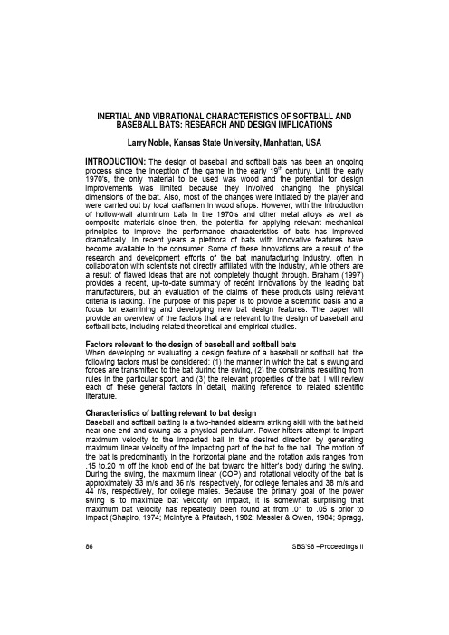
INERTIAL AND VIBRATIONAL CHARACTERISTICS OF SOFTBALL AND BASEBALL BATS: RESEARCH AND DESIGN IMPLICATIONSLarry Noble, Kansas State University, Manhattan, USA INTRODUCTION: The design of baseball and softball bats has been an ongoing process since the inception of the game in the early 19th century. Until the early 1970's, the only material to be used was wood and the potential for design improvements was limited because they involved changing the physical dimensions of the bat. Also, most of the changes were initiated by the player and were carried out by local craftsmen in wood shops. However, with the introduction of hollow-wall aluminum bats in the 1970's and other metal alloys as well as composite materials since then, the potential for applying relevant mechanical principles to improve the performance characteristics of bats has improved dramatically. In recent years a plethora of bats with innovative features have become available to the consumer. Some of these innovations are a result of the research and development efforts of the bat manufacturing industry, often in collaboration with scientists not directly affiliated with the industry, while others are a result of flawed ideas that are not completely thought through. Braham (1997) provides a recent, up-to-date summary of recent innovations by the leading bat manufacturers, but an evaluation of the claims of these products using relevant criteria is lacking. The purpose of this paper is to provide a scientific basis and a focus for examining and developing new bat design features. The paper will provide an overview of the factors that are relevant to the design of baseball and softball bats, including related theoretical and empirical studies.Factors relevant to the design of baseball and softball batsWhen developing or evaluating a design feature of a baseball or softball bat, the following factors must be considered: (1) the manner in which the bat is swung and forces are transmitted to the bat during the swing, (2) the constraints resulting from rules in the particular sport, and (3) the relevant properties of the bat. I will review each of these general factors in detail, making reference to related scientific literature.Characteristics of batting relevant to bat designBaseball and softball batting is a two-handed sidearm striking skill with the bat held near one end and swung as a physical pendulum. Power hitters attempt to impart maximum velocity to the impacted ball in the desired direction by generating maximum linear velocity of the impacting part of the bat to the ball. The motion of the bat is predominantly in the horizontal plane and the rotation axis ranges from .15 to.20 m off the knob end of the bat toward the hitter’s body during the swing. During the swing, the maximum linear (COP) and rotational velocity of the bat is approximately 33 m/s and 36 r/s, respectively, for college females and 38 m/s and 44 r/s, respectively, for college males. Because the primary goal of the power swing is to maximize bat velocity on impact, it is somewhat surprising that maximum bat velocity has repeatedly been found at from .01 to .05 s prior to impact (Shapiro, 1974; McIntyre & Pfautsch, 1982; Messier & Owen, 1984; Spragg, 86 ISBS'98 –Proceedings II1986). While this finding has been reported in the scientific literature frequently, a plausible explanation of the reason has not been found. A review of the elastic properties of the bat (appearing later in this paper) and the characteristics of the swing may provide a tenable hypothesis. It is possible that, at the beginning of the swing, torque applied to the bat handle to rotate the bat toward the incoming ball and the inertia of the barrel end of the bat cause the bat to bend, with the barrel of the bat lagging behind. This bending mode, usually referred to as the diving board mode , would begin to release when the rotational acceleration of the bat begins to drop. It is conjectured that the elite hitter learns through trial and error to adopt a bat and swing that are matched such that the velocity of the impact point of the bat is maximized at impact. To accomplish this end, accelerating forces would be reduced quickly at either 1/4 or 1 3/4 of the period of oscillation of the diving board mode. For example, if the fundamental, diving board mode of a bat is 25 Hz, then the period of oscillation is 40 ms. For the hitter to take advantage of this elastic behavior, this bending mode would need to be …released“ at approximately 10 or 70 ms prior to impact. While this characteristic of the skilled golf swing has been empirically verified (Cochran & Stobbs, 1986), no empirical data in support of this hypothesis applied to softball or baseball bats have been found.Rules most relevant to bat designThe rules regarding baseball bat characteristics are different from those regarding softball bats. Also, rules are different for different genders and different levels of play. For adult males, the maximum baseball and softball bat barrel size is 2.25 and 2.75 in (.057 and .070 m), respectively. The maximum bat length is 42 and 34 inches (1.067 and .864 m) for baseball and softball, respectively, while the maximum softball bat weight is 38 oz (10.569 N). There is no maximum baseball bat weight. All bats used in professional baseball must be made of wood. The most recent rule, which places an upper limit on the coefficient of restitution (Bat Performance Factor) for bats at different levels and types of play, is having a tremendous impact on the direction of bat design activity. Bat performance factor will be discussed in greater detail later in this paper.Inertial and vibrational properties relevant to bat designSeveral inertial and vibrational properties of the bat are relevant to its effective use: (1) mass, (2) moment of inertia, (3) coefficient of restitution, (4) location of node of the fundamental vibration node, and (5) center of percussion location.Mass and moment of inertia determine the amount of effort required to swing the bat. There is an inverse relationship between bat linear and angular acceleration and mass and moment of inertia, respectively, for a given linear and angular impulse (integral of force/torque and time). Thus, the more mass and/or moment of inertia, the more impulse required to produce a given change in bat speed or direction. In other words, greater mass and moment of inertia compromise the hitter’s ability to control the path of the bat as it moves toward the ball as well as to generate bat velocity during the swing. Theoretical models of the relationship between mass and impact parameters indicate that lighter bats than have been used by most skilled players would be more effective (Kirkpatrick, 1963; Adair, 1990). In a study which sought to empirically determine an individual’s ideal bat, this concept was supported (Bahill & Karnavas, 1991). Furthermore, bats now used by elite softball and baseball players are much lighter than they were 10 years ago. ISBS'98 – Proceedings II 87Bat manufacturers and retailers do not provide moment of inertia measurements with their products; however, moment of inertia is a critical design parameter and is also used to develop bat selection guidelines.When the ball and bat are impacted, during impact the bat behaves in some respects as a physical pendulum and in some respects as an elastic body. Taking both rigid-body and elastic properties into consideration, the best part of the bat on which to hit the ball is called the …sweet spot“. The …sweet spot“ is a general, nonscientific term, that means that the best overall results are obtained from impacts on this point. In other words, impacts on the sweet spot feel best to the hitter and results in imparting velocity to the ball are best. Or, in more precise terms, the sweet spot is the impact location where the transfer of energy from the bat to the ball is maximal while the transfer of energy to the hands is minimal. On closer examination, four parameters have been identified as having an effect on the …sweetness“ (liveliness) and location of the sweet spot: (1) center of percussion (COP), (2) node of the fundamental vibrational mode, (3) coefficient of restitution, and (4) the maximum …power“ point.Center of percussion. When the ball hits the bat at the center of percussion (COP), there is no reaction impulse (shock) at the axis. The impact axis for bats has been shown to be the point under the first knuckle of the top hand (Plagenhoef, 1971; Noble, 1983). Thus, COP impacts are more comfortable than at other locations because there is no painful impact …shock“ that is experienced during impacts at other locations. The distance from the impact axis to the COP of a bat can be found from the following equation:COP dist = T2g/4π2 = .2483877*T2 (units in meters)where T is the period of one oscillation when the bat is suspended from the axis, and g is the gravitational constant in meters. The COP has been demonstrated to be the impact location producing the greatest post-impact velocity with stationary bats (Weyrich, Messier, Ruhmann, & Berry, 1989). Another empirical study involving 18 elite slow-pitch softball hitters reported a correlation of .58 between the perceived location of the sweet spot and the COP. Thus, COP location explained 33% of the variability in perceived sweet spot impact location (Noble, 1983). Brody developed a theoretical construct for determining the impact location of a swinging bat with a pitched ball that would result in greatest postimpact ball velocity (Brody, 1986). This location was not on the COP, but was a function of the relative velocity and mass of the ball and bat as well as the inertial properties of the bat.In an early study (Bryant, Bryant, Chen, & Krahenbuhl, 1977) comparing the dynamic and performance characteristics of aluminum and wood bats, data were reported showing an impact area of several cm in length on hollow-wall aluminum bats where there was zero-order reaction impulse while reaction impulse on wood bats was a direct linear of function of distance from the COP. However, a later study by Noble and Eck (Noble & Eck, 1986) presented a theoretical construct and empirical data demonstrating that, assuming the bat is rigid during impact, reaction impulse is a direct linear function of the distance of the impact from the COP (Figure 1). Also, the slope of the regression line of impact reaction impulse on impact-COP distance is a direct linear function of the distance of the COP from the impact axis (Figure 2). In other words, the greater the distance of the COP from the 88 ISBS'98 –Proceedings IIISBS'98 – Proceedings II 89 hands, the smaller the reaction impulse resulting from an impact of a given distance from the COP. This study also demonstrated thatthe distance of the COP from the axis was:COP = I/Mrwhere I = moment of inertia about the axis, M = the totalbat mass, and r = distance from the axis to the center ofmass. Strategies were later presented for systematicallydisplacing the location of the COP (Noble & Eck, 1985) by placing mass at various locations along the longitudinalaxis of the bat. While these strategies were effectivein displacing the COP to a more distal location on the bat,this …improvement“ did not enjoy wide acceptance by theplayers because of the greater excitation of thefundamental vibrational mode resulting from COP impacts(Noble & Walker, 1994b).Figure 1. Mechanical system describing center of percussion (COP)location as a function of impact location. (Legend: P = impact impulse, P 1= impact reaction impulse, A = impact location, a p = distance from COMto COP, O = impact axis, M = mass, S = axis-COM distance, I o = momentof inertia about impact axis). Note. From …Effects of Selected Softball BatLoading Strategies on Impact Reaction Impulse“ by L. Noble and J. Eck(1986). Medicine and Science in Sports and Exercise 18, 51. Copyright1986 by the American College of Sports Medicine. Adapted with permission.Figure 2. Theoretical relationship between impact reaction impulse and impact location. (Legend: P = impact impulse, P 1 = impact reaction impulse, a p = COP location, a = distance from impact axis to impact, M = mass, S = axis-COM distance, I o = moment of inertia about impact axis). Note. From …Effects of Selected Softball Bat Loading Strategies on Impact Reaction Impulse“ by L. Noble and J. Eck (1986). Medicine and Science in Sports and Exercise 18, 51. Copyright 1986 by the American College of Sports Medicine. Adapted with permission.90 ISBS'98 –Proceedings II Vibrational properties. The above discussion relates to the rigid body behavior of the bat during impact. The bat also exhibits important and relevant elastic properties during impact as well as during the swing because the bat is not completely rigid. The vibrational behavior of a bat approximates that of a uniform beam, described in detail in most engineering textbooks on vibrations (Thompson, 1993). If we assume, for simplicity, that a bat can be represented by a uniform rod rigidly suspended at the point of contact with the hands, then the various normal vibrational modes are only those for a rigid clamped rod. Figure 3a illustrates the approximate length (modeled after a uniform rod), node locations, and relative amplitude of these modes. The lowest frequency mode, commonly called the diving board mode, corresponds to a vibration where the axis is at a nodal point and the barrel end is at a maximum. This node has a wavelength (λ0)of approximately 4H, where H is the distance from the axis to the barrel end of the bat. This fundamental mode only has one node and it is located at the clamped point. The next highest frequency mode has a node at the handle and another at 3/4H. If the ball strikes the bat at a node of a given vibrational mode, then thatmode will not be excited. Since all modes have an anti-node at theFigure 3. Vibrational modes of bat as (a) a uniformed rod clamped at the axis, and (b) as a free-free rod. (λi = approximate wavelength of i th harmonic modeled as a uniform rod). Note: Part a from …Effects of Selected Softball Bat Loading Strategies on Impact Reaction Impulse“ by L. Noble and J. Eck (1986). Medicine and Science in Sports and Exercise 18, 51. Copyright 1986 by the American College of Sports Medicine. Part b from …Baseball Bat Inertial and vibrational Characteristics and Discomfort Following Ball-Bat Impacts“ by L. Noble and H. Walker (1994). Journal of Applied Biomechanics 10,134. Copyright 1994 by Human Kinetics, Inc. Adapted with permission.unclamped, or barrel end of the bat, all modes of vibration can be excited when striking the bat at the barrel end. The frequency of the diving board mode has been reported to be 27 Hz for an aluminum softball bat and 18 Hz for a wood softball bat (Brody, 1990) and that of the first overtone mode was 317 and 209 Hz, respectively. Both of these bats were 34 inches (.864 m) in length. Shorter bats and bats with greater strength/mass ratios will have higher fundamental frequencies. It is likely that this mode is excited during the swing, as has been demonstrated during the swinging of golf clubs (Cochran & Stobbs, 1986); however, this low-frequency mode is not excited by the impacting ball (Brody, 1990; Noble & Walker, 1994a; Noble & Walker, 1994b).During impact, the vibration behavior of the bat corresponds to that of a free, non-supported bat whether irregardless of the firmness of the grip. Figure 3b illustrates the lowest (fundamental) and first harmonic modes, approximate wavelengths and node locations of the free, unsupported bat. The approximate locations of the two nodes for the first mode are 29% of the bat length from each end. The next highest mode has three nodes with approximate locations as depicted in Figure 3b. The number of nodes for each successively higher mode increases by one at each step. Also, the amplitude associated with each mode decreases as the frequency increases and increases as the distance from the node increases.The node locations and frequency of the fundamental and first harmonic modes can be measured by, first, supporting the bat in a horizontal position by threads attached to the ceiling. A vibration exciter and velocity sensor are horizontally oriented and placed as indicated in Figure 4. Specific placement of the exciter and sensor is not critical as long as they are not placed on one of the nodes. A resister is put in series with the exciter coil, and the voltage displayed on the horizontal axis of an oscilloscope. This voltage is proportional to the current through the resister and exciter coil which is proportional to the force applied by the exciter. The output of the velocity sensor is displayed on the vertical axis of the oscilloscope. This display is generally an ellipse whose axes are oriented at an angle determined by the gain setting of the oscilloscope, the phase relationship of the two signals, and the location of the velocity sensor. The input is gradually increased in frequency until resonance is achieved. At resonance, the exciting force and velocity are in phase and the ellipse is reduced to a straight line. The straight line changes slope as the velocity sensor is moved along the long axis of the bat. The slope changes from positive to negative as the sensor passes over a node and is horizontal when the sensor is located at a node.ISBS'98 – Proceedings II 91The fundamental frequency (free condition) of 34-inch (.864m) aluminum softball bats is usually within the range of 180-360 Hz and can be varied throughout this range by changing the shape of the bat and strategic redistribution of mass (Noble & Walker, 1993). The easiest way to change the fundamental frequency is to modify the diameter of the bat in the taper region, which is near the antinode of theFigure 4. Vibration measurement system. From …Baseball Bat Inertial and vibrational Characteristics and Discomfort Following Ball-Bat Impacts“ by L. Noble, H. Walker (1994). Journal of Applied Biomechanics10, 134. Copyright 1994 by Human Kinetics, Inc. Adapted with permission. fundamental mode. Node locations of the fundamental mode can also be strategically displaced as much as .06 mm using similar strategies. The distal node of the fundamental mode has been identified as one of the determinants of the sweet spot. Impacts on the node do not excite the low-frequency, fundamental mode, resulting in a higher-frequency sound and smaller, higher frequency vibrations of the bat handle. Thus, it is reasonable to expect that nodal impacts would be more comfortable for the hitter. Fortunately, in most bats the location of this node and the COP are less than .02 m apart, approximately 25 per cent of the bat length from the barrel end. When using bats with the node and COP close together, impacts at both locations are more comfortable than at other locations (Noble & Walker, 1994a) with no significant difference between the two. However, strategies developed to strategically displace the COP toward the barrel end were found to significantly increase the distance (.06 m) between the node and COP. Impacts at the node on these bats were found to be more comfortable than impacts at any other location, including the COP (Noble & Walker, 1994b). This is consistent with results from a study investigating the sweet spot location of tennis racquets indicating the node as the predominant predictor of sweet spot location (Hatze, 1994). Furthermore, the node-COP distance has been found to be one of the most powerful predictors of player’s perception of bat performance and preference (Noble & Dzewaltowski, 1994).No empirical studies have been found investigating the effects of impact location relative to the location of the distal node of the fundamental mode on post-impact ball velocity. However, an excellent theoretical presentation of this effect has been developed, but unfortunately it remains unpublished (Van Zandt, 1991). This paper applied the theory of the elastic behavior of an irregularly shaped, cylindrically92 ISBS'98 –Proceedings IIsymmetric object to a wood baseball bat (frequency of diving board mode and first harmonic - 27 Hz and 137 Hz, respectively). The node-COP distance was .01 m. A set of equations was developed and used to find the first 20 normal modes of vibration and calculate each mode’s effect on the recoil of the ball. Figure 5 illustrates estimates of the post-impact ball velocity as a function of impact point along the length of the bat. The impact ball and bat velocities were 40 m/sec and 16 m/sec, respectively. The solid curve shows the expected result, the dashed curve shows the effect of suppressing all modes above the fundamental for the free condition (137 Hz), and the starred curve shows the performance expected for an infinitely rigid club having otherwise identical properties. Two observations relative to the effect of impact location and post-impact ball velocity are notable: (1) post-impact velocity is significantly lower for impacts not on the node, especially as the impact location moves toward the handle of the bat; and (2) the higher-frequency modes serve to increase post-impact ball velocity. For a collision only .10 m toward the bat handle from the node, post-impact ball velocity is expected to decrease by 5%. The effect of this loss in ball velocity would cost a distance in ball flight of 10%, or 42 ft (12.8 m). The higher elastic modes play an important role in bat performance, restoring approximately 50% of the loss in ball velocity. This degradation in bat performance would be less with stiffer bats with higher natural frequencies, such as those made from composites, aluminum, and other metal alloys. The loss in bat performance would be eliminated if the fundamental frequency of the bat was …tuned“ to the ball-bat contact, or dwell, time. To obtain impact frequency tuning, the fundamental frequency should equal the reciprocal of twice the dwell time. For example, the dwell time of a softball and bat collision (velocity = 31 m/s) has been measured at .0035 sec (Plagenhoef, 1971). For this case, the frequency-matched bat would have a fundamental frequency of 143 Hz. This procedure would be difficult to effectively apply with precision because the dwell time is a function of collision velocity, which is not entirely under the control of the hitter, as well as the hardness of the ball. Coefficient of restitution. The coefficient of restitution (COR) of two colliding objects, such as the ball and bat, is the ratio of the difference between their velocities immediately after impact compared to the difference between their velocities prior to impact. This ratio has been shown to be a function of collision velocity as well as temperature. For simplicity, the COR of balls and bats are evaluated separately. Ball COR is usually determined by impacting the balls with a wooden wall backed by concrete. Rules for different levels of play for softball and baseball have been established setting an upper limit for the COR, usually determined by impacting the balls with a steel plate at 60 mph (26.4 m/s). The COR is now often stamped on the cover of the ball. For most adult softball competition, the maximum COR is .55. The COR of bats has been shown to be a weak function of impact location along the barrel of the bat where the diameter is constant. Thus, it does not play a significant role in determining the location of the sweet spot. If a given ball impacts with a ball with these conditions held constant, the bat with the higher coefficient of restitution will produce the greatest post- impact ball velocity. Improving the COR of bats has been the primary focus of the research and development efforts of the major bat manufacturers during the past decade. The COR has been significantly improved through the use of materials of higher strength/mass ratios and strategic manipulation of the wall thickness of the ISBS'98 – Proceedings II 93barrel of the bat. These dramatic increases in COR have caused great concern on the part of coaches and officials associated with all levels of play. This concern relates to the safety of the participants and to the changes in the nature and integrity of the games that those associated with the game identify with. An outgrowth of this concern is the adoption of a standard for evaluating theFigure 5. Theoretical estimates of the degradation of post-impact ball velocity at different impact locations due to bat vibrations. From The Dynamical Theory of the Baseball Bat, by L. L. Van Zandt (1991). Unpublished manuscript. W. Lafayette, IN: Purdue University.…liveliness“ (COR) of bats and implementing rules placing an upper limit on this aspect of bat performance. A standard method of testing to measure the COR of bats has recently been adopted by most of the baseball and rules committees in the USA (ASTM, 1995). This procedure involves impacting a ball with a known COR with a stationary bat with a fixed axis (free to rotate) at the bat’s COP at a ball speed of 88 ft/sec (26.8 m/s). The COR is calculated by the standard method of comparing the difference between the velocity of the bat and ball before impact to that following impact. A Bat Performance Factor (BPF) is then calculated from the ratio of bat and ball COR to the ball COR. For example, if the predetermined ball COR is .5 and the measured COR of the ball-bat collision is .55, then the BPFof the bat would be 1.1. The BPF of most wood bats is between .9 and 1.0 whilethat of the latest aluminum alloy bats is typically above 1.1. Maximum bat94 ISBS'98 –Proceedings IIperformance standards have now been adopted by most levels of play for both baseball and softball. For example, the maximum BPF allowed for most adult slow pitch softball is 1.2 and that established for collegiate baseball is 1.15. The adoption of this standard has changed the recent trend in bat design from focusing on increasing COR to improving other performance characteristics that comply with the rules.Maximum …power“ point. The impact point along the longitudinal axis of the bat that will result in the greatest post-impact ball velocity, or maximum power point, is another important performance characteristic of the bat. Brody (1986) developed a theoretical framework and estimates of the maximum power point for a bat that is swung and impacts with a pitched ball, behaving as a free-free body during impact. Estimates of the location of the distance from the maximum power point to the bat COM (PPTDIST) were found to increase as the mass and moment of inertia of the bat increases and as the ratio of bat/ball mass increases. Furthermore, PPTDIST increases as the ratio of bat angular velocity to ball linear velocity increases. Thus, PPTDIST was estimated to be less for baseball than for fastpitch softball. PPTDIST was calculated for an aluminum softball bat and ball with varying bat/ball velocity and mass ratios and found the location of the maximum power point to be located between the COM and COP. No empirical data relative to these estimates was reported. Weyrich, Messier, Ruhmann (1989) provided empirical data on the effects of impact location on postimpact ball velocity. Bats were not swung, but held stationary by either clamps or strings mounted to the ceiling while balls were propelled against the bat at 27 m/s. Impacts on the COP produced greater postimpact ball velocities than impacts on the COM and impacts near the barrel end. While these results are apparently contradictory to the theoretical work of Brody(1986), these bats were not swung, as Brody’s estimates assume, and no impacts were studied in the area between the COM and COP. The empirical data provided by Noble (1983) in an earlier study does, however, appear to conflict with Brody’s estimates. In this study, the location of 52 self-perceived …sweet spot“ impacts of 12 elite male softball players and 5 highly skilled college male baseball players was examined using cinematographic methods (200 f/s). The …sweet spot“ location, the point where the results were best, coincided very closely with the COP location. Furthermore, sweet spot location relative to the COP did not appear to be different for softball and baseball impacts. If it can be assumed that these elite players’ perception of sweet spot is synonymous with the maximum power point, then these results do not seem to support Brody’s 1986) theoretical estimates of maximum power point location. However, because COP location only accounted for 33 per cent of the variability in sweet spot location in the empirical study (Noble, 1983), other characteristics of the bat, ball, hitter-bat interface and of the swing probably affected these results. Further empirical research is necessary to clarify this issue. CONCLUSIONS: Several important factors relevant to the design of baseball and softball bats were identified.: (1) how is the bat swung and how forces are transmitted to the bat during the swing, (2) what are the constraints resulting from rules in the particular sport, and (3) what mechanical properties are relevant. The most important mechanical properties of the bat are: (1) mass, (2) moment of inertia, (3) coefficient of restitution (COR), (4) vibrational properties, (5) center of ISBS'98 – Proceedings II 95。

The sweet spot-2010MCM paper.

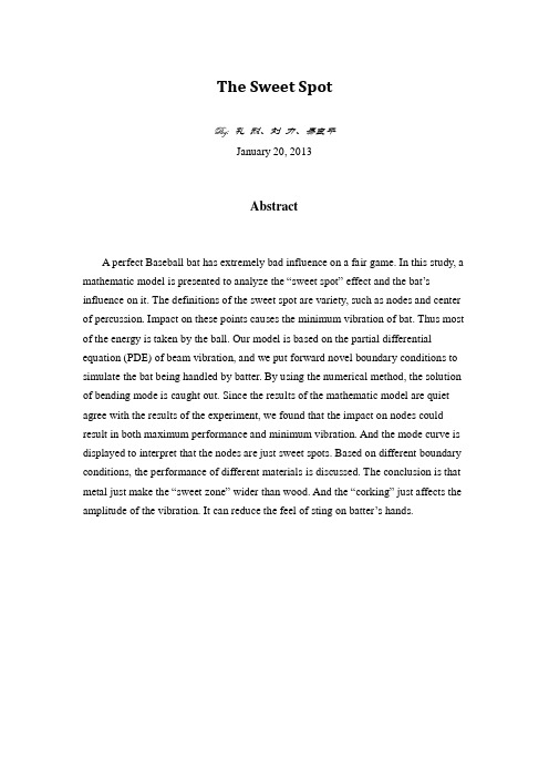
List of Figures
Fig. 1 Mode Shapes for the Prismatic Wood Beam ............................................... 11 Fig. 2 Mode Shapes for the Prismatic Wood Beam ............................................... 11 Fig. 3 Mode Shapes for the Prismatic Aluminum Beam ....................................... 12 Fig. 4 Mode Shape Comparison between the Prismatic Hollow Aluminum Beam and Prismatic Wood Beam .......................................................................... 13 Fig. 5 Cork in a Bat .................................................................................................. 14 Fig. 6 Superposition of Wood Mode Shapes .......................................................... 14
Contents
Abstract............................................................................................................... 1 1 Introduction ................................................................................................... 3 1.1 Notation and Definitions ..................................................................... 3 1.2 Brief Explanations of the Sweet Spot ................................................. 4 1.3 Energy Model ....................................................................................... 5 1.4 General Assumptions ........................................................................... 5 2 Vibration Model ............................................................................................ 6 2.1 Outline of Vibration Model ............................................................... 6 2.2 The Partial Differential Equation...................................................... 6 3 Method Descriptions .................................................................................... 9 3.1 Simplification ....................................................................................... 9 3.2 Bending Mode Analysis .................................................................... 10 4 Results and Interpretations ......................................................................... 10 4.1 Why isn’t the sweet spot at the end of the bat? ............................... 10 4.2 How does the material work?............................................................ 12 4.3 Corking?............................................................................................. of Model ....................................................... 15 References ........................................................................................................ 15

MCM ICM 数学建模优秀论文石油资源模型

ቤተ መጻሕፍቲ ባይዱ
Introduction
The United States per capita GNP (gross national product) rose bk a factor of 7.5 between 1870 and 1980. The fuel for such unparalleled growth was petroleum. Nonrenewable fuels now supply almost 90% of the energy produced domestically. But petroleum is a nonrenewable resource, with a limited supply. And we have used almost half of the world's total supply, demand is increasing, and world production will soon peak. In 1956, near the height of the growth rate of the U.S. oil industry, geologist M.K. Hubbert drew a bell-shaped curve to depict production of oil in the U.S. over the coming decades. With remarkable accuracy, even despite a large unforeseen find in'Alaska, Hubbert correctly predicted domestic oil production would peak in 1970. In 1989, the United States imported more fuel than it produced domestically; currently, it gets 60% of its fuel from imports. However, the lack of recent discoveries is even more disconcerting. We have already located over 1,600 billion barrels of oil in the world, whether already produced or still underground. If we accept the preferred estimate of 1,800 billion barrels as the total amount of oil recoverable-for a profit, then we have only 200 billion barrels left to discover, which will only add about 20% to our current reserves. Many people believe that once oil prices rise high enough due to scarcity, it will be profitable for oil companies to harvest reserves that are not yet economically viable However, there is something else more prevalent here than the price in dollars: the price in energy. In Hubbert's own words, "When the energy cost of recovering a barrel of oil becomes greater than the energy content of the oil, production will cease no matter what the monetary price may be" [Ecosystems 2005]. The fundamental question is, How long will our oil supply last? World production is predicted to peak between 2000 and 2020. The world supply can be expected to run out between 40 and 60 years from now. Our model addresses depletion of oil over a long horizon by using historical data from 1930 onward. This model is flexible enough to account for almost any economic, political, and natural factors.

美赛优秀论文2010MCM的B特等奖翻译

摘要：该模型最大的挑战是如何建立连环杀手犯罪行为的模型。

因为找出受害者之间的联系是非常困难的；因此，我们预测罪犯的下一个目标地点，而不是具体目标是谁。

这种预测一个罪犯的犯罪的空间格局叫做犯罪空间情报分析。

研究表明：最暴力的连环杀手的犯罪范围一般在一个径向带中央点附近：例如家庭，办公室，以及其他一些犯罪行为高发区（例如城镇妓女集中区）。

这些‘锚点’为我们的模型提供了基础。

我们假设整个分析域是一个潜在的犯罪现场。

罪犯的活动不受到任何条件约束；并且该区域足够大包括所有的打击点。

我们考虑的是一个可度量的空间，为预测算法创建了空间可能性。

此外；我们假设罪犯为一个暴力的系列犯罪者，因为研究表明窃贼和纵火犯不可能遵循某一空间模式。

一个锚点与多个锚点有着实质性的不同，首先讨论单个锚点的案例，建立坐标系并把罪犯最后犯罪地点与犯罪序列表示出来，并估计以前案件发生地地点，评估模型的可靠性，并且我们得到未来可能发生犯罪行为的锚点。

对于多个锚点的案例，我们通过聚类与排序的方法：将所给数据划分为几组。

在每组中找一个最重要的锚点，每一个分区都给定一个权值。

我们进行单点测试，利用以前的锚点预测最近的一个锚点，并且与其实际位置相比较。

我们从文献中摘录七个数据集，并且用其中四个改善我们的模型，检测其序列变化，地理集中位置和总锚点的数目。

然后通过其他三点来评估我们的模型。

结果显示多个锚点的模型的结果比较优。

引言：通过研究文献中以得出的连环案件罪犯地理空间往往是围绕罪犯日常活动的几个锚点附近的区域。

我们建立的预测模型就是在其规律下建立的，并且预测出一个表面的可能值和度量值。

第一个方案是通过重心法寻找出单个可能的锚点。

第二个方案是假设2到4个锚点，并且利用聚类算法的排序与分组的方法。

两种方案都是利用统计方法来缩小预测未来犯罪的地点区域背景：1981年peter sutcliffe的逮捕是法医生物学家stuart kind 通过利用数理原理成功预测出约克郡开膛手的住处的一个标志目前，信息密集型模型是通过热图技术建立确定特殊犯罪类型的热点或者是找出犯罪活动与某一地区之间的联系比率。

1、下载文档前请自行甄别文档内容的完整性，平台不提供额外的编辑、内容补充、找答案等附加服务。
2、"仅部分预览"的文档,不可在线预览部分如存在完整性等问题,可反馈申请退款(可完整预览的文档不适用该条件!)。
3、如文档侵犯您的权益，请联系客服反馈,我们会尽快为您处理(人工客服工作时间：9:00-18:30)。

For the second problem, using Rayleigh distribution function, we obtain a preliminary probability distribution of the crime site based on the residence determined in the ﬁrst problem . Taking geographical character and the offender’s geographical preference into account, we utilize cluster analysis to divide all the crime sites into 4 zones. In these 4 zones, we construct 4 two-dimensional normal distributions around the 4 circle centers with the standard deviations being the radii of the circles. In view of the inﬂuence of the crime time, we add a time factor to the preliminary distribution. As a result, the preliminary distribution is modulated by geographical and temporal factors, producing an ultimate prediction, which is rather satisfactory after validation.
3 Center of Minimum Distance Model.................................. 5
3.1 Notations ........................................................................ 5 3.2 Simplifying Assumptions.................................................... 6 3.3 Center of Minimum Distance Model ..................................... 6 3.4 Case Study....................................................................... 6
7 Validation of Prediction...................................................... 20 8 Evaluating of Solutions ....................................................Chief of Police ........................ 22
9.1 Preparatory Work.............................................................. 22 9.2 Overview of the Potential Issues........................................... 22 9.3 Suggestion ....................................................................... 23
For the ﬁrst problem, based on the least effort principle, we build the Center of Minimum Distance Model and obtain the possible residence area of the criminal. Then based on Bayes’ Theorem and Rayleigh distribution function, we build the Bayesian Model and get another possible residence area. After that, we design a technique of using a minimum circle to cover the two areas to combine the two schemes.
2 Problem Analysis ............................................................... 4
2.1 Overall Strategy ................................................................ 4 2.2 The Strategies for Problem I................................................. 4 2.3 The Strategy for Problem II ................................................. 4
8.1 Strengths ......................................................................... 20 8.2 Weaknesses...................................................................... 21 8.3 Future Consideration ......................................................... 21
References ................................................................................. 24
2
Team #7120
page3 of 24
1 Introduction
1.1 Background
Serial crimes have a serious effect on people’s lives and continuously challenge people’s baseline of morality. Thus, how to arrest the criminals before he or she commits another crime becomes an important issue. A number of sophisticated techniques have been developed to generate a useful prediction for law enforcement ofﬁcers based on the time and locations of the past crime scenes, such as the “center of a mass” method.
1.1 Background ..................................................................... 3 1.2 Geographic Proﬁling.......................................................... 3 1.3 Objectives........................................................................ 3
4 Bayesian Model .................................................................. 9
4.1 Notations and Deﬁnitions ................................................... 9 4.2 Simplifying Assumptions.................................................... 10 4.3 Bayesian Model ................................................................ 10 4.4 Case Study....................................................................... 12 4.5 The Discussion of α............................................................ 12
Finally, an executive summary is presented for law enforcement ofﬁcers.
Contents
Summary ................................................................................... 1 1 Introduction ....................................................................... 3
5 Combination of the Results of the Two Schemes................ 13 6 Prediction of the Next Crime.............................................. 14