AnsysWorkbench-15-Fluent 流体 管道 初级教程 示例-合并
ansys fluent中文版流体计算工程案例详解
ansys fluent中文版流体计算工程案例详解ANSYS Fluent是一种流体计算动力学软件,可用于解决各种流体力学问题。
本文将详细介绍ANSYS Fluent中文版的流体计算工程案例,包括案例的基本背景、模拟过程和结果分析。
这些案例旨在帮助用户深入了解ANSYS Fluent的使用方法和流体计算工程实践。
一个典型的案例是流体在管道中的流动。
该案例背景是,一根长直管道内有水流动,管道的直径为0.1米,长度为10米。
水的初始速度为1 m/s,管道的壁面是光滑的,管道两端的压差为100Pa。
现在需要使用ANSYS Fluent模拟该流体流动过程,并进一步分析不同参数对流动的影响。
首先,在ANSYS Fluent中创建一个新的仿真项目,并选择“仿真”模块。
在界面上点击“新建”按钮,在弹出的对话框中填写相应的参数,例如案例名称、计算器类型和尺寸单位。
点击“确定”后,进入模拟设置页面。
首先,需要定义获得流动场稳定解所需的物理模型和求解方法。
在“物理模型”选项卡中,选择“连续相”和“非恒定模型”。
在“湍流模型”中选择某种适合的模型,例如k-ε模型。
在“重力”选项卡中,定义流体的密度和重力加速度。
接下来,在“模型”选项卡中,定义管道的几何和边界条件。
选择“管道”作为流体领域的几何模型,并定义长度、直径和内壁面的润滑系数。
在“边界”选项卡中,定义管道两端的入口和出口条件,例如速度和压力。
将管道两端的压力差设置为100Pa,在入口处设置水的初始速度为1 m/s。
在出口处选择“出流”边界条件。
完成几何和边界条件的定义后,点击“模拟”选项卡进入模拟设置界面。
在“求解控制”中,设置计算时间步长和迭代次数。
选择合适的网格划分方法,并进行网格划分。
点击“网格”选项卡,选择合适的网格类型,并进行网格划分。
在划分网格后,可以使用“导入”按钮导入网格文件,并进行网格优化。
完成设置后,点击“计算”按钮开始进行模拟计算。
在计算过程中,可以实时观察流体场的变化情况,并通过Fluent Post-processing工具进行结果分析。
旋流器fluent数值模拟ANSYS15.0
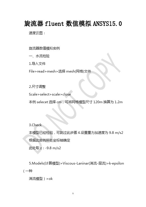
旋流器fluent数值模拟ANSYS15.0速度云图:旋流器数值模拟实例一、水流检验1.导入文件File>read>mesh>选择mesh(网格)文件2.尺寸调整Scale>select>scale>close本例selecet选择cm,可将网格模型尺寸120m换算为1.2m3.Check本模型已经检验,可跳过此步骤4.设置重力加速度为9.8 m/s2 根据此实例所处坐标轴确定此处取z:-9.8 m/s25.Models(计算模型)>Viscous-Laninar(湍流-层流)>k-epsilon (一种湍流模型)>ok本实例为大锥角旋流器,矿浆加压给入,流体类型为湍流;k-epsilon适合完全发展的湍流,对雷诺数较低的过渡情况和近壁区域计算的不好。
6.Materials(材料性质)>Fluid>FluentDatabase(流体数据库)>water-liquid(水介质流)>copy>close7.Cell Zone Conditious>fluid>water-liquid>okCell Zone Conditious单元区域条件,在建立网格模型(mesh)时,将旋流器内部腔体划分为多个体积微元,即此步骤设置的是体积微元数值模拟的介质是水流。
8.BoundaryConditions>pressure_inlet.2>Edit>Momentum>输入6>ok设置边界条件,“pressure_inter.2”为建立网格模型时设置的入口边界条件,类型为压力入口,在此,改为速度入口,速度设置为6 m/s。
9.如图仿照7.将pressure_topoutlet.3和underoutlet 的“Type”设置为pressure_outlet,不编辑数值点OK结束此步。
10.S olution Initialization>Standard Initialization> pressure_inlet.2>Initialization此步为数值的初始化设置,图片和描述不符以上述文字为准。
ansys fluent中文版流体计算工程案例详解

ansys fluent中文版流体计算工程案例详解ANSYS Fluent是一种用于计算流体力学的软件,通过数值模拟的方式进行流体分析和设计。
在实际应用中,需要使用流体计算工程案例来验证仿真结果的准确性和可靠性。
下面将介绍一些常见的应用案例。
1.汽车空气动力学设计。
在汽车设计中,空气动力学是一个非常重要的因素。
使用ANSYS Fluent可以对汽车外形进行流体分析,如气流、气压、气动力等。
通过对气流的模拟,可以优化车身外形设计,提高汽车的性能和燃油经济性。
2.船舶流场分析。
船舶的流体设计是提高船舶速度和燃油经济性的重要因素。
使用ANSYS Fluent可以对船舶外形和水动力性能进行分析。
通过模拟船舶在水中的流动情况,可以优化船体外形和螺旋桨设计,提高航行效率。
3.风力发电机设计。
风力发电机是一种通过风力发电的机械设备。
通过ANSYS Fluent对风场进行数值模拟,可以预测风力发电机的性能和稳定性。
通过分析叶片的气动力学特性,可以优化叶片的设计,提高风力发电机的发电效率。
4.石油钻井液流分析。
石油钻井过程中,需要注入液体来冷却钻头并加速岩屑的排除。
使用ANSYS Fluent对液体的流动情况进行数值模拟,可以预测液体的流动速度和压降,优化钻井液的配比,提高钻井效率。
5.医用注射器设计。
医用注射器是一种常见的医疗器械。
通过使用ANSYS Fluent分析注射器的流场,可以优化注射器的设计。
通过预测注射器注射药液时的速度和压降,可以优化注射器的内部结构和开孔位置,提高注射的精度和安全性。
总之,ANSYS Fluent可以应用于各种流体力学领域,帮助工程师们进行流体力学设计与分析,取得更高效准确的结果。
这些案例都为设计和实施各种流体系统提供了指导,可以大大提高工作效率。
ANSYS CFD管道流体分析经典算例 Fluid

Fluid #2: Velocity analysis of fluid flow in a channel USING FLOTRAN Introduction:In this example you will model fluid flow in a channelPhysical Problem:Compute and plot the velocity distribution within the elbow. Assume that the flow is uniform at both the inlet and the outlet sections and that the elbow has uniform depth.Problem Description:T he channel has dimensions as shown in the figureThe flow velocity as the inlet is 10 cm/sUse the continuity equation to compute the flow velocity at exitObjective:T o plot the velocity profile in the channelT o plot the velocity profile across the elbowYou are required to hand in print outs for the aboveFigure:IMPORTANT: Convert all dimensions and forces into SI unitsSTARTING ANSYSC lick on ANSYS 6.1in the programs menu.S elect Interactive.T he following menu comes up. Enter the working directory. All your files will be stored in this directory. Also under UseDefault Memory Model make sure the values 64 for Total Workspace, and 32 for Database are entered. To change these values unclick Use Default Memory ModelMODELING THE STRUCTUREG o to the ANSYS Utility Menu (the top bar)Click Workplane>W P Settings…The following window comes up:o Check the Cartesian and Grid Only buttonso Enter the values shown in the figure aboveGo to the ANSYS Main Menu (on the left hand side of the screen) and click Preprocessor>Modeling>Create>Keypoints>On Working PlaneCreate keypoints corresponding to the vertices in the figure. The keypoints look like below.Now create lines joining these key points.M odeling>Create>Lines>Lines>Straight lineT he model looks like the one below.Now create fillets between lines L4-L5 and L1-L2.C lick Modeling>Create>Lines>Line Fillet. A pop-up window will now appear. Select lines 4 and 5. Click OK. The following window will appear:T his window assigns the fillet radius. Set this value to 0.1 m.Repeat this process of filleting for Lines 1 and 2.The model should look like this now:N ow make an area enclosed by these lines.M odeling>Create>Areas>Arbitrary>By LinesS elect all the lines and click OK. The model looks like the followingT he modeling of the problem is done.ELEMENT PROPERTIESSELECTING ELEMENT TYPE:Click Preprocessor>Element Type>Add/Edit/Delete... In the 'Element Types' window that opens click on Add... The following window opens.∙Type 1 in the Element type reference number.∙Click on Flotran CFD and select 2D Flotran 141. Click OK. Close the Element types window.∙So now we have selected Element type 1 to be solved using Flotran, the computational fluid dynamics portion of ANSYS. This finishes the selection of element type.DEFINE THE FLUID PROPERTIES:∙Go to Preprocessor>Flotran Set Up>Fluid Properties.∙On the box, shown below, set the first two input fields as Air-SI, and then click on OK. Another box will appear. Accept the default values by clicking OK.∙Now we’re ready to define the Material PropertiesMATERIAL PROPERTIESW e will model the fluid flow problem as a thermal conduction problem. The flow corresponds to heat flux, pressurecorresponds to temperature difference and permeability corresponds to conductance.Go to the ANSYS Main MenuClick Preprocessor>Material Props>Material Models. The following window will appearA s displayed, choose CFD>Density. The following window appears.F ill in 1.23 to set the density of Air. Click OK.Now choose CFD>Viscosity. The following window appears:N ow the Material 1 has the properties defined in the above table so the Material Models window may be closed.MESHING: DIVIDING THE CHANNEL INTO ELEMENTS:G o to Preprocessor>Meshing>Size Cntrls>ManualSize>Lines>All Lines.I n the window that comes up type 0.01 in the field for 'Element edge length'.N ow Click OK.Now go to Preprocessor>Meshing>Mesh>Areas>Free. Click the area and the OK. The mesh will look like thefollowing.BOUNDARY CONDITIONS AND CONSTRAINTSG o to Preprocessor>Loads>Define Loads>Apply>Fluid CFD>Velocity>On lines. Pick the left edge of theouter block and Click OK. The following window comes up.E nter 0.1 in the VX value field and click OK. The 0.1 corresponds to the velocity of 0.1 meter per second of air flowingfrom the left side.R epeat the above and set the Velocity to ZERO for the air along all of the edges of the pipe. (VX=VY=0 for all sides)O nce they have been applied, the pipe will look like this:∙Go to Main Menu>Preprocessor>Loads>Define Loads>Apply>Fluid CFD>Pressure DOF>On Lines.∙Pick the outlet line. (The horizontal line at the top of the area) Click OK.∙Enter 0 for the Pressure value.∙Now the Modeling of the problem is done.SOLUTIONG o to ANSYS Main Menu>Solution>Flotran Set Up>Execution Ctrl.∙The following window appears. Change the first input field value to 300, as shown. No other changes are needed. Click OK.G o to Solution>Run FLOTRAN.W ait for ANSYS to solve the problem.C lick on OK and close the 'Information' window.POST-PROCESSINGP lotting the velocity distribution…Go to General Postproc>Read Results>Last Set.Then go to General Postproc>Plot Results>Contour Plot>Nodal Solution. The following window appears:∙Select DOF Solution and Velocity VSUM and Click OK.∙This is what the solution should look like:∙Next, go to Main Menu>General Postproc>Plot Results>Vector Plot>Predefined.The following window will appear:∙Select OK to accept the defaults. This will display the vector plot to compare to the solution of the same tutorial solved using the Heat Flux analogy. Note: This analysis is FAR more precise as shown by the followingsolution:∙Go to Main Menu>General Postproc>Path Operations>Define Path>By Nodes∙Pick points at the ends of the elbow as shown. We will graph the velocity distribution along the line joiningthese two points.∙The following window comes up.∙Enter the values as shown.∙Now go to Main Menu>General Postproc>Path Operations>Map onto Path. The following window comes up.∙Now go to Main Menu>General Postproc>Path Operations>Plot Path Items>On Graph.∙The following window comes up.∙Select VELOCITY and click OK.∙The graph will look as follows:。
使用AnsysFluent进行流体力学仿真教程
使用AnsysFluent进行流体力学仿真教程Chapter 1: Introduction to ANSYS FluentIn this chapter, we will provide an overview of ANSYS Fluent and explain its importance in the field of fluid dynamics simulation. ANSYS Fluent is a powerful computational fluid dynamics (CFD) software used for simulating and analyzing fluid flows. It enables engineers and scientists to study the behavior of fluids, predict their performance in various scenarios, and optimize the design of systems involving fluid flow.Chapter 2: Pre-ProcessingThe pre-processing stage involves preparing the geometry of the system and defining the desired fluid flow conditions. ANSYS Fluent provides a variety of tools to import and manipulate geometry files, such as creating boundaries, defining initial conditions, and specifying material properties. Additionally, it allows users to create a mesh grid that discretizes the computational domain into smaller elements for accurate simulations.Chapter 3: Boundary ConditionsBoundary conditions play a crucial role in defining the behavior of the fluid flow simulation. In this chapter, we will explain the different types of boundary conditions available in ANSYS Fluent, including velocity inlet, pressure outlet, wall, and symmetry. Each boundarycondition has specific input parameters that need to be defined, such as velocity magnitude, pressure, and temperature.Chapter 4: Solver SettingsThe solver settings determine the numerical methods used to solve the fluid flow equations in ANSYS Fluent. This chapter will introduce the various solver options available, including pressure-based and density-based solvers. It will also discuss the importance of convergence criteria and the influence of physical properties, such as turbulence models and turbulence intensity.Chapter 5: Post-ProcessingOnce the simulation is complete, post-processing is performed to analyze and visualize the results. In ANSYS Fluent, users have access to a range of post-processing tools, such as contour plots, vector plots, velocity profiles, and pressure distribution. This chapter will explain how to interpret these results to gain insights into the fluid flow behavior and make informed design decisions.Chapter 6: Advanced FeaturesIn this chapter, we will explore some of the advanced features of ANSYS Fluent that can enhance the accuracy and efficiency of fluid flow simulations. These include multiphase flow simulations, combustion modeling, heat transfer analysis, and turbulence modeling. We will provide step-by-step instructions on how to set up and run simulations using these advanced features.Chapter 7: Case StudiesTo further illustrate the capabilities of ANSYS Fluent, this chapter will present a series of case studies involving different fluid flow scenarios. These case studies will cover a range of applications, such as fluid flow in pipes, aerodynamics of a car, and natural convection in a room. Each case study will include the problem statement, simulation setup, and analysis of the results.Chapter 8: Troubleshooting and TipsANYS Fluent, like any software, can sometimes encounter issues or produce unexpected results. In this chapter, we will discuss common troubleshooting techniques and provide tips for optimizing simulation setup and improving simulation accuracy. This will include techniques for mesh refinement, convergence improvement, and understanding error messages.Conclusion:ANSYS Fluent is a powerful tool for conducting fluid dynamics simulations. In this tutorial, we have covered the fundamental aspectsof using ANSYS Fluent, including pre-processing, boundary conditions, solver settings, post-processing, advanced features, and troubleshooting. By following this tutorial, users can gain a solid foundation in conducting fluid flow simulations using ANSYS Fluent and leverageits capabilities to analyze and optimize fluid flow systems in various applications.。
AnsysWorkbench_15_Fluent示例-3
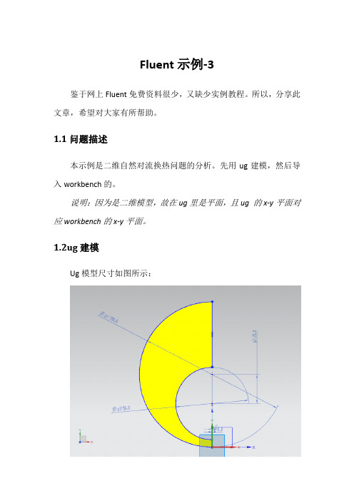
Fluent示例-3鉴于网上Fluent免费资料很少,又缺少实例教程。
所以,分享此文章,希望对大家有所帮助。
1.1问题描述本示例是二维自然对流换热问题的分析。
先用ug建模,然后导入workbench的。
说明:因为是二维模型,故在ug里是平面,且ug 的x-y平面对应workbench的x-y平面。
1.2ug建模Ug模型尺寸如图所示:首先在workbench中建立FLUENT工程,如下图所示。
、说明:这是我的分析过程。
如果是新建的话,是没有那么多“对号”的。
当每完成一个步骤,才会有对号出现。
左键选中Geometry后,右键单击,会出现一快捷菜单,选Import 后,浏览所建立的模型,点击OK后,自动打开DM窗口,别忘了左键单击Generate,才能显示导入的模型。
导入workbench后的模型如下图所示:Workbench中的mesh设置如下(这是示例,所以比较简单)。
其他可以默认。
完成设置后,单击Generate Mesh按钮,完成分网。
1.5打开FLUENT截面如图所示1.5.1 General设置比例如下,别忘点击Scale。
说明,一般情况下,点击一次。
1.5.2 Models设置如下图所示,打开能量方程。
1.5.3 Materials设置双击air,打开对话框,设置如下如下图所示:说明:zone 中的如”wall_in 、wall_out”实在workbench 中DM 或Mesh 后取的名,目的是便于选择。
方法为右击要定义的线,弹出的菜单中选择有“Name ”的命令,然后命名即可。
1.5.5 Solution Methods 设置:如下图所示;1.5.6 Monitors设置如下图所示:1.5.7 Gravity设置在菜单Define中选择Operating Condition,打开对话框,设置如下1.5.8 Solution Initialization设置如下图所示设置循环迭代200次,最后,点击计算。
学会使用ANSYSFluent进行流体力学模拟和分析
学会使用ANSYSFluent进行流体力学模拟和分析流体力学是研究流体运动和相互作用的科学。
在工程学领域,流体力学广泛应用于模拟和分析各种工程问题,如气体和液体流动、热传递、质量传递等。
而ANSYSFluent是一种常用的流体力学模拟和分析软件,可以帮助工程师和科研人员进行流体力学模型的建立、仿真和结果分析。
本文将介绍如何学会使用ANSYSFluent进行流体力学模拟和分析。
第一章:ANSYSFluent简介ANSYSFluent是面向工程领域的一款强大的计算流体力学软件。
它提供了广泛的模型和分析工具,可以模拟和分析各种流体力学问题。
ANSYSFluent具有友好的界面,简单易用,同时也具备高级的功能和定制性。
该软件在汽车、航空、化工等领域得到了广泛的应用。
第二章:流体力学模拟流程在使用ANSYSFluent进行流体力学模拟和分析之前,我们需要先了解整个模拟流程。
首先,我们需要定义几何模型,可以通过导入CAD模型或手动构建几何体。
然后,对几何模型进行网格划分,将其离散成小的单元。
接下来,设置流体材料的物性参数,如密度、粘度和热传导系数。
然后,定义流体动力学模型,如流动方程和边界条件。
最后,进行求解和后处理,通过数值方法求解流体力学方程,并分析结果。
第三章:几何建模在ANSYSFluent中,我们可以使用多种方法进行几何建模。
一种常用的方法是通过导入CAD模型,可以直接打开各种常见格式的CAD文件。
另一种方法是使用Fluent的几何建模工具,可以手动构建几何体。
该工具提供了创建基本几何体(如圆柱、球体等)、布尔操作(如并集、交集等)和边界设置等功能,可以方便地生成复杂的几何体。
第四章:网格划分网格划分是流体力学模拟中的重要环节。
好的网格划分可以提高计算精度和计算效率。
在ANSYSFluent中,我们可以使用多种方法进行网格划分。
一种常用的方法是结构化网格划分,它将几何体划分成规则的网格单元。
另一种方法是非结构化网格划分,它允许在几何体中创建任意形状的网格单元。
2012-08-06 简单易学 图文并茂 ANSYS Work Bench FLUENT 入门

<简单易学> <图文并茂> ANSYS WB之Fluent入门**Fluent是流体仿真的高级工具,其能力有口皆碑,这里就不累述了。
WB中的Fluent,简化了以往建模和网格划分等环节,并且后处理也非常方便。
实际使用后,我觉得WB的Fluent 流程非常清晰。
所以特写此贴,方便以往没有接触过Fluent的朋友按图索骥。
备注:这个教程,基本和Fluent帮助的第一个算例非常相近,不清楚的地方可参看官方教程。
特别是一些关键的设置,可以通过帮助文件直接索引到技术文档。
**本例是一个三通的混液器,入口进来三种不同速度,不同温度的水。
先上最终的结果图(Q0)**三通管道是在ProE里创建的(Q1),可直接下载附件:threeinlet.prt.rar**通过ProE上方的AnsysWB菜单栏,直接进入WB(Q2)这是WB里出现“几何”模块。
双击进入“几何编辑器”**选择第一个“导入特征”,右键选择生成(Q3)。
**之后再编辑器中,生成几何形体(Q4)**然后再WB中,拖进来一个“Mesh”模块。
把几何连接到Mesh模块(Q5)**双击打开“Mesh”界面(Q6)**在Mesh模块中,进行必要的,针对流体网格划分的设置(Q7)1:从Outline的Mesh进入2:目标软件设置为CFD的Fluent3:Size部分按图设置4:特别是Inflation部分,Use Automatic Inflation设置为“Program Control”。
这样可以自动生成壁面层。
备注:流体的壁面层性质是非常特殊的,因此网格划分会专门考虑这点。
WB针对Fluent的自动网格划分,可在四面体网格基础上,走动生成壁面网格,速度非常快,质量也很不错。
虽然同六面体网格相比肯定不足,但对于简单的几何,已经非常理想了。
特别是现在电脑日新月异,即便较为复杂的几何,这种网格都是能算的,仅时间长点而已。
**后面这步很重要。
- 1、下载文档前请自行甄别文档内容的完整性,平台不提供额外的编辑、内容补充、找答案等附加服务。
- 2、"仅部分预览"的文档,不可在线预览部分如存在完整性等问题,可反馈申请退款(可完整预览的文档不适用该条件!)。
- 3、如文档侵犯您的权益,请联系客服反馈,我们会尽快为您处理(人工客服工作时间:9:00-18:30)。
Fluent示例鉴于网上Fluent免费资料很少,又缺少实例教程。
所以,分享此文章,希望对大家有所帮助。
1.1问题描述本示例为ansys-fluent15.0-指南中的,不过稍有改动。
1.2 Ug建模图1.3 Workbench设置项目设置如下图所示。
(为了凸显示例,所以个项目名称没改动;并且用两种添加项目方式分析,还增加了一个copy项,以供对比。
)说明:ansys workbench15.0与ug8.5(当然,也包括同一时期的solidworks、Pro/e等三维CAD软件)可无缝连接,支持ug8.5建立的模型,可直接导入到ansys workbench15.0中。
方法:在workbench中的Geometry点击右键,弹出快捷菜单,选择“browse”,浏览到以保存的文件,打开即可。
个人感觉workbench 建模不方便。
1.4 DM处理Workbench中的DM打开模型,将导入的模型在DM中切片处理,以减少分网、计算对电脑硬件的压力(处理大模型常用的方法,也可称之为技巧)。
最终效果,如下图所示。
为以后做Fluent方便,在这里要给感兴趣的面“取名”(最好是给每一个面都取名。
这样,便于后续操作)。
方法是右键所选择的面,在弹出的对话框中“添加名称”即可,给“面”取“名“成功后,会在左边的tree Outline中显示相应的“名”。
结果如下图所示(图中Symmetry有两个,有一个是错的,声明一下)1.5 Mesh设置如下图所示。
在Mesh中insert一个sizing项(右键Mesh,选Sizing即可),以便分体网格,其设置如下:分体网格的方法:先选择“体”,然后在Geometry中选择Apply 即可。
最后设置单元大小6e-3m。
1.6 setup设置如下图所示。
1.6.1Units设置选择General中的Units项,打开对话框,如下设置:选择好后,点击close后确认并关闭对话框。
说明:这样做显示较为细腻,缺点是需后续单位换算。
Fluent默认单位国际单位。
1.6.2 Models设置如下如所示,开启能量方程;双击Viscous选项,选择K-ε选项,并选择Enchanced wall Treatment模式。
说明:Enhanced Wall Treatment适合K-ε模型。
1.6.3 Material设置如下图,材料选择water。
说明:如果材料库中没有water,可手动添加。
方法:选择Fluent,然后选择Creat/Edit,改name为water,最后点击No。
(如果点击yes,则将把原有的材料-air改动了。
)Water参数如下说明,要记得单位换算。
1.6.4 Cell Zone Conditions设置如下图所示,选择相应的boundary设置如下:其余boundary默认。
1.6.6 Solution Methods设置如下图所示其余选项默认即可。
1.6.7 Montors设置如下图所示其中monitors栏,点选Edit后编辑,设置如下一般默认即可,不过还是看看吧。
Surface Monitors作用是显示所要“监视”的内容,设置方法如下:增加内容时选Creat,编辑已有内容时选Edit,删除已有内容时选Delete。
当选Creat时,可参考注意,Name是自动生成的,不用自己取名(当然,自己命名也无妨)。
Window内容是显示窗口的编号,一般按顺序增加即可。
Get Data Every为“写入频率”,采用默认值也可以。
Report Type是报告类型;Field Variable是“监视”内容,下拉菜单中的内容均可选择,关于它们名称解释可参考网络上的文章。
此对话框中的内容,按需选择即可。
本示例中“监视”内容为3个,方便演示。
1.6.8 Solution Initiation设置选择“混合模式”,最后点击Initiation初始化。
如下图所示1.6.9 Run Calculation设置包括“迭代次数”、“写入频率”等,最后Calculate即可,内容如下(本例迭代次数300——数值多少,自己定,其余默认即可)2.0 结果显示选择菜单中的Insert项,按需要添加即可。
举例,添加个contour,默认名称“contour1”,点击OK,添加成功。
接着,弹出对话框如下:其中Locations的下拉菜单为在DM中给面添加的名称;Variable为要“显示”的变量名;Range为变量范围,一般情况下选Global即可,其余项可取默认值。
选择完毕后,记得点击Apply才能显示。
本例结果如下:说明:1 不同分析平台,不同建模方法,结果会不一样。
2 本示例Fluent 求解过程中忘记截图了,所以没有求解过程和求解完毕的截图。
3 本示例只是表明fluent的一般求解过程,具体参数仅供参考(我直接取自“指南”中的了。
这样,省事)4 workbench中项目的建立,可直接选择Toolbox里面的,也可选择Custom System里面的,结果都一样。
Fluent示例-2鉴于网上Fluent免费资料很少,又缺少实例教程。
所以,分享此文章,希望对大家有所帮助。
1.1问题描述本示例为ansys-fluent15.0-指南中的,不过稍有改动。
1.2 Ug建模图1.3 分网Mesh图这里引用上一例子的mesh图,当然,也可重新划分网格,选用四面体等。
1.4 Fluent设置如图,打开Fluent,并设置,参考下图所示。
(一般情况下默认就行,当然,也可以自行设置,比如,文件存储位置等)1.5导入mesh文件导入上一例子的mesh文件。
方法,Fluent中的file—read----mesh 在打开的对话框中,浏览到指定文件,ok即可导入成功。
效果如下图。
选择General---mesh---scale,设置转换单位,下图只是举个例子动转换,而其他单位还是国际单位。
1.5.2 models设置如图所示,说明,双击Energy打开对话框,打上对号,ok即可确认和关闭对话框。
双击viscous打开对话框,如下图所示,进行设置。
1.5.3 材料material设置如下图所示,选择water项。
具体添加侧向方法,参阅上一例子。
1.5.4 cell zone conditions设置如下图所示,zone里面就一个选项,只能选它。
然后edited,打开对话框,如果单击edit打开下面的对话框,会显示所选材料属性。
可用来验证材料选择正确否。
1.5.5 Boundary Condition设置会显示如下图可参考上一例子的设置。
不过参数要准确,否则可能计算不收敛,或程序根本就不求解了。
一下给出本例的参考值。
其余默认即可。
1.5.6 Solution Method设置如下图所示,1.5.7 Monitor设置如下图所示说明,Monitors是监视器,Residential是残差设置,结果是在显示窗口上实时显示求解的残差曲线,计算收不收敛一看便知。
而Surface Monitors是监视有关平面的参数,单击Creat或Edit打开如下对话框说明,点击右侧的“黑倒三角”弹出下拉菜单,按需选择感兴趣的参数即可完成“监视设置”。
最后,一定要悬赏“Print to Console,和plot”两项,尤其是“plot”,否则,窗口不显示。
1.5.8 Solution Initiation设置这一般都会了,计算前都要初始化,目的是读入刚才设置的值。
如下图所示最后,初始化,点击Initialize。
1.5.9 Run Calculator设置设置循环步数,然后开始求解。
如下图1.6 Result设置可以参考按下图设置,查看结果可以点击左侧的Plot项,在弹出的对话框中设置相关参数,最后Display一下,就会出现点图结果。
举例如下图点击左侧的Report项,在弹出的对话框中进行设置,最后Computer一下,会出现结果。
举例如图说明,注意对话框中的results和Net Results,与文本框中显示的NET值相同(四舍五入后)。
重要提示流体流入为正;流体流出为负。
切记。
Fluent示例-3鉴于网上Fluent免费资料很少,又缺少实例教程。
所以,分享此文章,希望对大家有所帮助。
1.1问题描述本示例是二维自然对流换热问题的分析。
先用ug建模,然后导入workbench的。
说明:因为是二维模型,故在ug里是平面,且ug 的x-y平面对应workbench的x-y平面。
1.2ug建模Ug模型尺寸如图所示:首先在workbench中建立FLUENT工程,如下图所示。
、说明:这是我的分析过程。
如果是新建的话,是没有那么多“对号”的。
当每完成一个步骤,才会有对号出现。
左键选中Geometry后,右键单击,会出现一快捷菜单,选Import 后,浏览所建立的模型,点击OK后,自动打开DM窗口,别忘了左键单击Generate,才能显示导入的模型。
导入workbench后的模型如下图所示:Workbench中的mesh设置如下(这是示例,所以比较简单)。
其他可以默认。
完成设置后,单击Generate Mesh按钮,完成分网。
1.5打开FLUENT截面如图所示1.5.1 General设置比例如下,别忘点击Scale。
说明,一般情况下,点击一次。