陆振波SVM的MATLAB代码解释
matlab的svmrfe函数

一、介绍MATLAB是一种流行的技术计算软件,广泛应用于工程、科学和其他领域。
在MATLAB的工具箱中,包含了许多函数和工具,可以帮助用户解决各种问题。
其中,SVMRFE函数是MATLAB中的一个重要功能,用于支持向量机分类问题中的特征选择。
二、SVMRFE函数的作用SVMRFE函数的全称为Support Vector Machines Recursive Feature Elimination,它的作用是利用支持向量机进行特征选择。
在机器学习和模式识别领域,特征选择是一项重要的任务,通过选择最重要的特征,可以提高分类器的性能,并且减少计算和存储的开销。
特征选择问题在实际应用中经常遇到,例如在生物信息学中,选择基因表达数据中最相关的基因;在图像处理中,选择最相关的像素特征。
SVMRFE函数可以自动化地解决这些问题,帮助用户找到最佳的特征子集。
三、使用SVMRFE函数使用SVMRFE函数,用户需要准备好特征矩阵X和目标变量y,其中X是大小为m×n的矩阵,表示m个样本的n个特征;y是大小为m×1的向量,表示m个样本的类别标签。
用户还需要设置支持向量机的参数,如惩罚参数C和核函数类型等。
接下来,用户可以调用SVMRFE函数,设置特征选择的方法、评价指标以及其他参数。
SVMRFE函数将自动进行特征选择,并返回最佳的特征子集,以及相应的评价指标。
用户可以根据返回的结果,进行后续的分类器训练和预测。
四、SVMRFE函数的优点SVMRFE函数具有以下几个优点:1. 自动化:SVMRFE函数可以自动选择最佳的特征子集,减少了用户手工试验的时间和精力。
2. 高性能:SVMRFE函数采用支持向量机作为分类器,具有较高的分类精度和泛化能力。
3. 灵活性:SVMRFE函数支持多种特征选择方法和评价指标,用户可以根据自己的需求进行灵活调整。
五、SVMRFE函数的示例以下是一个简单的示例,演示了如何使用SVMRFE函数进行特征选择:```matlab准备数据load fisheririsX = meas;y = species;设置参数opts.method = 'rfe';opts.nf = 2;调用SVMRFE函数[selected, evals] = svmrfe(X, y, opts);```在这个示例中,我们使用了鸢尾花数据集,设置了特征选择的方法为递归特征消除(RFE),并且要选择2个特征。
支持向量机(SVM)算法的matlab的实现
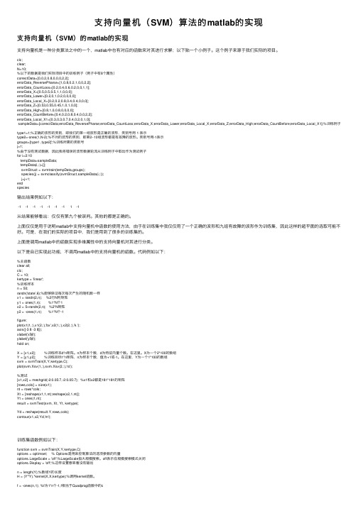
⽀持向量机(SVM)算法的matlab的实现⽀持向量机(SVM)的matlab的实现⽀持向量机是⼀种分类算法之中的⼀个,matlab中也有对应的函数来对其进⾏求解;以下贴⼀个⼩例⼦。
这个例⼦来源于我们实际的项⽬。
clc;clear;N=10;%以下的数据是我们实际项⽬中的训练例⼦(例⼦中有8个属性)correctData=[0,0.2,0.8,0,0,0,2,2];errorData_ReversePharse=[1,0.8,0.2,1,0,0,2,2];errorData_CountLoss=[0.2,0.4,0.6,0.2,0,0,1,1];errorData_X=[0.5,0.5,0.5,1,1,0,0,0];errorData_Lower=[0.2,0,1,0.2,0,0,0,0];errorData_Local_X=[0.2,0.2,0.8,0.4,0.4,0,0,0];errorData_Z=[0.53,0.55,0.45,1,0,1,0,0];errorData_High=[0.8,1,0,0.8,0,0,0,0];errorData_CountBefore=[0.4,0.2,0.8,0.4,0,0,2,2];errorData_Local_X1=[0.3,0.3,0.7,0.4,0.2,0,1,0];sampleData=[correctData;errorData_ReversePharse;errorData_CountLoss;errorData_X;errorData_Lower;errorData_Local_X;errorData_Z;errorData_High;errorData_CountBefore;errorData_Local_X1];%训练例⼦type1=1;%正确的波形的类别,即我们的第⼀组波形是正确的波形,类别号⽤ 1 表⽰type2=-ones(1,N-2);%不对的波形的类别,即第2~10组波形都是有故障的波形。
支持向量机matlab实现源代码知识讲解

支持向量机m a t l a b 实现源代码edit svmtrain>>edit svmclassify>>edit svmpredictfunction [svm_struct, svIndex] = svmtrain(training, groupnames, varargin)%SVMTRAIN trains a support vector machine classifier%% SVMStruct = SVMTRAIN(TRAINING,GROUP) trains a support vector machine % classifier using data TRAINING taken from two groups given by GROUP.% SVMStruct contains information about the trained classifier that is% used by SVMCLASSIFY for classification. GROUP is a column vector of% values of the same length as TRAINING that defines two groups. Each% element of GROUP specifies the group the corresponding row of TRAINING % belongs to. GROUP can be a numeric vector, a string array, or a cell% array of strings. SVMTRAIN treats NaNs or empty strings in GROUP as% missing values and ignores the corresponding rows of TRAINING.%% SVMTRAIN(...,'KERNEL_FUNCTION',KFUN) allows you to specify the kernel % function KFUN used to map the training data into kernel space. The% default kernel function is the dot product. KFUN can be one of the% following strings or a function handle:%% 'linear' Linear kernel or dot product% 'quadratic' Quadratic kernel% 'polynomial' Polynomial kernel (default order 3)% 'rbf' Gaussian Radial Basis Function kernel% 'mlp' Multilayer Perceptron kernel (default scale 1)% function A kernel function specified using @,% for example @KFUN, or an anonymous function%% A kernel function must be of the form%% function K = KFUN(U, V)%% The returned value, K, is a matrix of size M-by-N, where U and V have M% and N rows respectively. If KFUN is parameterized, you can use% anonymous functions to capture the problem-dependent parameters. For% example, suppose that your kernel function is%% function k = kfun(u,v,p1,p2)% k = tanh(p1*(u*v')+p2);%% You can set values for p1 and p2 and then use an anonymous function:% @(u,v) kfun(u,v,p1,p2).%% SVMTRAIN(...,'POLYORDER',ORDER) allows you to specify the order of a% polynomial kernel. The default order is 3.%% SVMTRAIN(...,'MLP_PARAMS',[P1 P2]) allows you to specify the% parameters of the Multilayer Perceptron (mlp) kernel. The mlp kernel% requires two parameters, P1 and P2, where K = tanh(P1*U*V' + P2) and P1% > 0 and P2 < 0. Default values are P1 = 1 and P2 = -1.%% SVMTRAIN(...,'METHOD',METHOD) allows you to specify the method used% to find the separating hyperplane. Options are%% 'QP' Use quadratic programming (requires the Optimization Toolbox)% 'LS' Use least-squares method%% If you have the Optimization Toolbox, then the QP method is the default% method. If not, the only available method is LS.%% SVMTRAIN(...,'QUADPROG_OPTS',OPTIONS) allows you to pass an OPTIONS % structure created using OPTIMSET to the QUADPROG function when using% the 'QP' method. See help optimset for more details.%% SVMTRAIN(...,'SHOWPLOT',true), when used with two-dimensional data,% creates a plot of the grouped data and plots the separating line for% the classifier.%% Example:% % Load the data and select features for classification% load fisheriris% data = [meas(:,1), meas(:,2)];% % Extract the Setosa class% groups = ismember(species,'setosa');% % Randomly select training and test sets% [train, test] = crossvalind('holdOut',groups);% cp = classperf(groups);% % Use a linear support vector machine classifier% svmStruct = svmtrain(data(train,:),groups(train),'showplot',true);% classes = svmclassify(svmStruct,data(test,:),'showplot',true);% % See how well the classifier performed% classperf(cp,classes,test);% cp.CorrectRate%% See also CLASSIFY, KNNCLASSIFY, QUADPROG, SVMCLASSIFY.% Copyright 2004 The MathWorks, Inc.% $Revision: 1.1.12.1 $ $Date: 2004/12/24 20:43:35 $% References:% [1] Kecman, V, Learning and Soft Computing,% MIT Press, Cambridge, MA. 2001.% [2] Suykens, J.A.K., Van Gestel, T., De Brabanter, J., De Moor, B.,% Vandewalle, J., Least Squares Support Vector Machines,% World Scientific, Singapore, 2002.% [3] Scholkopf, B., Smola, A.J., Learning with Kernels,% MIT Press, Cambridge, MA. 2002.%% SVMTRAIN(...,'KFUNARGS',ARGS) allows you to pass additional% arguments to kernel functions.% set defaultsplotflag = false;qp_opts = [];kfunargs = {};setPoly = false; usePoly = false;setMLP = false; useMLP = false;if ~isempty(which('quadprog'))useQuadprog = true;elseuseQuadprog = false;end% set default kernel functionkfun = @linear_kernel;% check inputsif nargin < 2error(nargchk(2,Inf,nargin))endnumoptargs = nargin -2;optargs = varargin;% grp2idx sorts a numeric grouping var ascending, and a string grouping % var by order of first occurrence[g,groupString] = grp2idx(groupnames);% check group is a vector -- though char input is special...if ~isvector(groupnames) && ~ischar(groupnames)error('Bioinfo:svmtrain:GroupNotVector',...'Group must be a vector.');end% make sure that the data is correctly oriented.if size(groupnames,1) == 1groupnames = groupnames';end% make sure data is the right sizen = length(groupnames);if size(training,1) ~= nif size(training,2) == ntraining = training';elseerror('Bioinfo:svmtrain:DataGroupSizeMismatch',...'GROUP and TRAINING must have the same number of rows.')endend% NaNs are treated as unknown classes and are removed from the training% datanans = find(isnan(g));if length(nans) > 0training(nans,:) = [];g(nans) = [];endngroups = length(groupString);if ngroups > 2error('Bioinfo:svmtrain:TooManyGroups',...'SVMTRAIN only supports classification into two groups.\nGROUP contains %d different groups.',ngroups) end% convert to 1, -1.g = 1 - (2* (g-1));% handle optional argumentsif numoptargs >= 1if rem(numoptargs,2)== 1error('Bioinfo:svmtrain:IncorrectNumberOfArguments',...'Incorrect number of arguments to %s.',mfilename);okargs = {'kernel_function','method','showplot','kfunargs','quadprog_opts','polyorder','mlp_params'}; for j=1:2:numoptargspname = optargs{j};pval = optargs{j+1};k = strmatch(lower(pname), okargs);%#okif isempty(k)error('Bioinfo:svmtrain:UnknownParameterName',...'Unknown parameter name: %s.',pname);elseif length(k)>1error('Bioinfo:svmtrain:AmbiguousParameterName',...'Ambiguous parameter name: %s.',pname);elseswitch(k)case 1 % kernel_functionif ischar(pval)okfuns = {'linear','quadratic',...'radial','rbf','polynomial','mlp'};funNum = strmatch(lower(pval), okfuns);%#okif isempty(funNum)funNum = 0;endswitch funNum %maybe make this less strict in the futurecase 1kfun = @linear_kernel;case 2kfun = @quadratic_kernel;case {3,4}kfun = @rbf_kernel;case 5kfun = @poly_kernel;usePoly = true;case 6kfun = @mlp_kernel;useMLP = true;otherwiseerror('Bioinfo:svmtrain:UnknownKernelFunction',...'Unknown Kernel Function %s.',kfun);endelseif isa (pval, 'function_handle')kfun = pval;elseerror('Bioinfo:svmtrain:BadKernelFunction',...'The kernel function input does not appear to be a function handle\nor valid function name.')case 2 % methodif strncmpi(pval,'qp',2)useQuadprog = true;if isempty(which('quadprog'))warning('Bioinfo:svmtrain:NoOptim',...'The Optimization Toolbox is required to use the quadratic programming method.') useQuadprog = false;endelseif strncmpi(pval,'ls',2)useQuadprog = false;elseerror('Bioinfo:svmtrain:UnknownMethod',...'Unknown method option %s. Valid methods are ''QP'' and ''LS''',pval);endcase 3 % displayif pval ~= 0if size(training,2) == 2plotflag = true;elsewarning('Bioinfo:svmtrain:OnlyPlot2D',...'The display option can only plot 2D training data.')endendcase 4 % kfunargsif iscell(pval)kfunargs = pval;elsekfunargs = {pval};endcase 5 % quadprog_optsif isstruct(pval)qp_opts = pval;elseif iscell(pval)qp_opts = optimset(pval{:});elseerror('Bioinfo:svmtrain:BadQuadprogOpts',...'QUADPROG_OPTS must be an opts structure.');endcase 6 % polyorderif ~isscalar(pval) || ~isnumeric(pval)error('Bioinfo:svmtrain:BadPolyOrder',...'POLYORDER must be a scalar value.');endif pval ~=floor(pval) || pval < 1error('Bioinfo:svmtrain:PolyOrderNotInt',...'The order of the polynomial kernel must be a positive integer.')endkfunargs = {pval};setPoly = true;case 7 % mlpparamsif numel(pval)~=2error('Bioinfo:svmtrain:BadMLPParams',...'MLP_PARAMS must be a two element array.');endif ~isscalar(pval(1)) || ~isscalar(pval(2))error('Bioinfo:svmtrain:MLPParamsNotScalar',...'The parameters of the multi-layer perceptron kernel must be scalar.'); endkfunargs = {pval(1),pval(2)};setMLP = true;endendendendif setPoly && ~usePolywarning('Bioinfo:svmtrain:PolyOrderNotPolyKernel',...'You specified a polynomial order but not a polynomial kernel');endif setMLP && ~useMLPwarning('Bioinfo:svmtrain:MLPParamNotMLPKernel',...'You specified MLP parameters but not an MLP kernel');end% plot the data if requestedif plotflag[hAxis,hLines] = svmplotdata(training,g);legend(hLines,cellstr(groupString));end% calculate kernel functiontrykx = feval(kfun,training,training,kfunargs{:});% ensure function is symmetrickx = (kx+kx')/2;catcherror('Bioinfo:svmtrain:UnknownKernelFunction',...'Error calculating the kernel function:\n%s\n', lasterr);end% create Hessian% add small constant eye to force stabilityH =((g*g').*kx) + sqrt(eps(class(training)))*eye(n);if useQuadprog% The large scale solver cannot handle this type of problem, so turn it% off.qp_opts = optimset(qp_opts,'LargeScale','Off');% X=QUADPROG(H,f,A,b,Aeq,beq,LB,UB,X0,opts)alpha = quadprog(H,-ones(n,1),[],[],...g',0,zeros(n,1),inf *ones(n,1),zeros(n,1),qp_opts);% The support vectors are the non-zeros of alphasvIndex = find(alpha > sqrt(eps));sv = training(svIndex,:);% calculate the parameters of the separating line from the support% vectors.alphaHat = g(svIndex).*alpha(svIndex);% Calculate the bias by applying the indicator function to the support% vector with largest alpha.[maxAlpha,maxPos] = max(alpha); %#okbias = g(maxPos) - sum(alphaHat.*kx(svIndex,maxPos));% an alternative method is to average the values over all support vectors % bias = mean(g(sv)' - sum(alphaHat(:,ones(1,numSVs)).*kx(sv,sv)));% An alternative way to calculate support vectors is to look for zeros of % the Lagrangians (fifth output from QUADPROG).%% [alpha,fval,output,exitflag,t] = quadprog(H,-ones(n,1),[],[],...% g',0,zeros(n,1),inf *ones(n,1),zeros(n,1),opts);%% sv = t.lower < sqrt(eps) & t.upper < sqrt(eps);else % Least-Squares% now build up compound matrix for solverA = [0 g';g,H];b = [0;ones(size(g))];x = A\b;% calculate the parameters of the separating line from the support % vectors.sv = training;bias = x(1);alphaHat = g.*x(2:end);endsvm_struct.SupportVectors = sv;svm_struct.Alpha = alphaHat;svm_struct.Bias = bias;svm_struct.KernelFunction = kfun;svm_struct.KernelFunctionArgs = kfunargs;svm_struct.GroupNames = groupnames;svm_struct.FigureHandles = [];if plotflaghSV = svmplotsvs(hAxis,svm_struct);svm_struct.FigureHandles = {hAxis,hLines,hSV};end。
LSSVM相关教程

四种支持向量机用于函数拟合与模式识别的Matlab示例程序陆振波点这里下载:四种支持向量机用于函数拟合与模式识别的Matlab示例程序使用要点:应研学论坛《人工智能与模式识别》版主magic_217之约,写一个关于针对初学者的《四种支持向量机工具箱》的详细使用说明。
同时也不断有网友向我反映看不懂我的源代码,以及询问如何将该工具箱应用到实际数据分析等问题,其中有相当一部分网友并不了解模式识别的基本概念,就急于使用这个工具箱。
本文从模式识别的基本概念谈起,过渡到神经网络模式识别,逐步引入到这四种支持向量机工具箱的使用。
本文适合没有模式识别基础,而又急于上手的初学者。
作者水平有限,欢迎同行批评指正![1]模式识别基本概念模式识别的方法有很多,常用有:贝叶斯决策、神经网络、支持向量机等等。
特别说明的是,本文所谈及的模式识别是指“有师分类”,即事先知道训练样本所属的类别,然后设计分类器,再用该分类器对测试样本进行识别,比较测试样本的实际所属类别与分类器输出的类别,进而统计正确识别率。
正确识别率是反映分类器性能的主要指标。
分类器的设计虽然是模式识别重要一环,但是样本的特征提取才是模式识别最关键的环节。
试想如果特征矢量不能有效地描述原样本,那么即使分类设计得再好也无法实现正确分类。
工程中我们所遇到的样本一般是一维矢量,如:语音信号,或者是二维矩阵,如:图片等。
特征提取就是将一维矢量或二维矩阵转化成一个维数比较低的特征矢量,该特征矢量用于分类器的输入。
关于特征提取,在各专业领域中也是一个重要的研究方向,如语音信号的谐振峰特征提取,图片的PCA特征提取等等。
[2]神经网络模式识别神经网络模式识别的基本原理是,神经网络可以任意逼近一个多维输入输出函数。
以三类分类:I、II、III为例,神经网络输入是样本的特征矢量,三类样本的神经网络输出可以是[1;0;0]、[0;1;0]、[0;0;1],也可以是[1;-1;-1]、[-1;1;-1]、[-1;-1;1]。
(1)matlab中SVM工具箱的使用方法
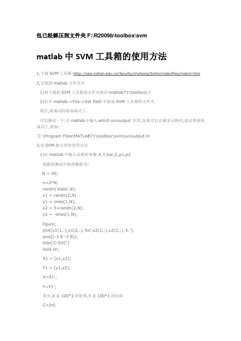
包已经解压到文件夹F:\R2009b\toolbox\svmmatlab中SVM工具箱的使用方法1,下载SVM工具箱:/faculty/chzheng/bishe/indexfiles/indexl.htm 2,安装到matlab文件夹中1)将下载的SVM工具箱的文件夹放在\matlab71\toolbox\下2)打开matlab->File->Set Path中添加SVM工具箱的文件夹现在,就成功的添加成功了.可以测试一下:在matlab中输入which svcoutput 回车,如果可以正确显示路径,就证明添加成功了,例如:C:\Program Files\MATLAB71\toolbox\svm\svcoutput.m3,用SVM做分类的使用方法1)在matlab中输入必要的参数:X,Y,ker,C,p1,p2我做的测试中取的数据为:N = 50;n=2*N;randn('state',6);x1 = randn(2,N)y1 = ones(1,N);x2 = 5+randn(2,N);y2 = -ones(1,N);figure;plot(x1(1,:),x1(2,:),'bx',x2(1,:),x2(2,:),'k.');axis([-3 8 -3 8]);title('C-SVC')hold on;X1 = [x1,x2];Y1 = [y1,y2];X=X1';Y=Y1';其中,X是100*2的矩阵,Y是100*1的矩阵C=Inf;ker='linear';global p1 p2p1=3;p2=1;然后,在matlab中输入:[nsv alpha bias] = svc(X,Y,ker,C),回车之后,会显示:Support Vector Classification_____________________________Constructing ...Optimising ...Execution time: 1.9 secondsStatus : OPTIMAL_SOLUTION|w0|^2 : 0.418414Margin : 3.091912Sum alpha : 0.418414Support Vectors : 3 (3.0%)nsv =3alpha =0.00000.00000.00000.00000.00002)输入预测函数,可以得到与预想的分类结果进行比较.输入:predictedY = svcoutput(X,Y,X,ker,alpha,bias),回车后得到:predictedY =1111111113)画图输入:svcplot(X,Y,ker,alpha,bias),回车补充:X和Y为数据,m*n:m为样本数,n为特征向量数比如:取20组训练数据X,10组有故障,10组无故障的,每个训练数据有13个特征参数,则m=20,n=13Y为20*1的矩阵,其中,10组为1,10组为-1.对于测试数据中,如果取6组测试数据,3组有故障,3组无故障的,则m=6,n=13Y中,m=6,n=1/SV M_soft.htmlSVM - Support Vector MachinesSoftwareTrain support vector machine classifier/access/helpdesk/help/toolbox/bioinfo/ref/svmtrain.html一些问题???????1.今天我在使用SVM通用工具箱对眼电的信号数据进行分类时出现如下错误:Support Vector Classification_____________________________Constructing ...Optimising ...??? Dimension error (arg 3 and later).Error in ==> svc at 60[alpha lambda how] = qp(H, c, A, b, vlb, vub, x0, neqcstr);不知道是什么原因?答:今天上午终于找到出现这一错误的原因:它并不是SVM程序的问题,是我在整理样本时,把参数需要的样本行列颠倒所致。
SVM多分类问题libsvm在matlab中的应用

SVM多分类问题libsvm在matlab中的应⽤转载⾃对于⽀持向量机,其是⼀个⼆类分类器,但是对于多分类,SVM也可以实现。
主要⽅法就是训练多个⼆类分类器。
⼀、多分类⽅式1、⼀对所有(One-Versus-All OVA)给定m个类,需要训练m个⼆类分类器。
其中的分类器 i 是将 i 类数据设置为类1(正类),其它所有m-1个i类以外的类共同设置为类2(负类),这样,针对每⼀个类都需要训练⼀个⼆类分类器,最后,我们⼀共有 m 个分类器。
对于⼀个需要分类的数据 x,将使⽤投票的⽅式来确定x的类别。
⽐如分类器 i 对数据 x 进⾏预测,如果获得的是正类结果,就说明⽤分类器 i 对 x 进⾏分类的结果是: x 属于 i 类,那么,类i获得⼀票。
如果获得的是负类结果,那说明 x 属于 i 类以外的其他类,那么,除 i 以外的每个类都获得⼀票。
最后统计得票最多的类,将是x的类属性。
2、所有对所有(All-Versus-All AVA)给定m个类,对m个类中的每两个类都训练⼀个分类器,总共的⼆类分类器个数为 m(m-1)/2 .⽐如有三个类,1,2,3,那么需要有三个分类器,分别是针对:1和2类,1和3类,2和3类。
对于⼀个需要分类的数据x,它需要经过所有分类器的预测,也同样使⽤投票的⽅式来决定x最终的类属性。
但是,此⽅法与”⼀对所有”⽅法相⽐,需要的分类器较多,并且因为在分类预测时,可能存在多个类票数相同的情况,从⽽使得数据x属于多个类别,影响分类精度。
对于多分类在matlab中的实现来说,matlab⾃带的svm分类函数只能使⽤函数实现⼆分类,多分类问题不能直接解决,需要根据上⾯提到的多分类的⽅法,⾃⼰实现。
虽然matlab⾃带的函数不能直接解决多酚类问题,但是我们可以应⽤libsvm⼯具包。
libsvm⼯具包采⽤第⼆种“多对多”的⽅法来直接实现多分类,可以解决的分类问题(包括C- SVC、n - SVC )、回归问题(包括e - SVR、n - SVR )以及分布估计(one-class-SVM )等,并提供了线性、多项式、径向基和S形函数四种常⽤的核函数供选择。
SVMmatlab代码详解说明

SVMmatlab 代码详解说明1234567891011x=[0 1 0 1 2 -1];y=[0 0 1 1 2 -1];z=[-1 1 1 -1 1 1]; %其中,(x,y )代表二维的数据点,z 表示相应点的类型属性。
data=[1,0;0,1;2,2;-1,-1;0,0;1,1];% (x,y)构成的数据点 groups=[1;1;1;1;-1;-1];%各个数据点的标签 figure; subplot(2,2,1); Struct1 = svmtrain(data,groups,'Kernel_Function','quadratic', 'showplot',true);%data 数据,标签,核函数,训练 classes1=svmclassify(Struct1,data,'showplot',true);%data 数据分类,并显示图形 title('二次核函数'); CorrectRate1=sum(groups==classes1)/6123456789101112131415subplot(2,2,2); Struct2 = svmtrain(data,groups,'Kernel_Function','rbf', 'RBF_Sigma',0.41,'showplot',true); classes2=svmclassify(Struct2,data,'showplot',true); title('高斯径向基核函数(核宽0.41)'); CorrectRate2=sum(groups==classes2)/6 subplot(2,2,3); Struct3 = svmtrain(data,groups,'Kernel_Function','polynomial', 'showplot',true); classes3=svmclassify(Struct3,data,'showplot',true); title('多项式核函数'); CorrectRate3=sum(groups==classes3)/6 subplot(2,2,4); Struct4 = svmtrain(data,groups,'Kernel_Function','mlp', 'showplot',true); classes4=svmclassify(Struct4,data,'showplot',true); title('多层感知机核函数');CorrectRate4=sum(groups==classes4)/61 <br><br><br>1 2 3 svmtrain 代码分析:if plotflag %画出训练数据的点[hAxis,hLines] = svmplotdata(training,groupIndex);4 5 6 7 8 9 10 11 12 13 14 15 16 17 18 19 20legend(hLines,cellstr(groupString)); endscaleData = [];if autoScale %训练数据标准化 scaleData.shift = - mean(training); stdVals = std(training); scaleData.scaleFactor = 1./stdVals; % leave zero-variance data unscaled: scaleData.scaleFactor(~isfinite(scaleData.scaleFactor)) = 1; % shift and scale columns of data matrix: for c = 1:size(training, 2) training(:,c) = scaleData.scaleFactor(c) * ... (training(:,c) + scaleData.shift(c)); end end1 2 3 if strcmpi(optimMethod, 'SMO')%选择最优化算法 else % QP and LS both need the kernel matrix: %求解出超平面的参数 (w,b): wX+b1 2 3 4 if plotflag %画出超平面在二维空间中的投影 hSV = svmplotsvs(hAxis,hLines,groupString,svm_struct); svm_struct.FigureHandles = {hAxis,hLines,hSV}; end1 s vmplotsvs.m 文件<br><br>1 2 3 4 5 6 7 hSV = plot(sv(:,1),sv(:,2),'ko');%从训练数据中选出支持向量,加上圈标记出来lims = axis(hAxis);%获取子图的坐标空间 [X,Y] = meshgrid(linspace(lims(1),lims(2)),linspace(lims(3),lims(4)));%根据x 和y 的范围,切分成网格,默认100份 Xorig = X; Yorig = Y;8 9 10 11 12 13 % need to scale the mesh 将这些隔点标准化 if ~isempty(scaleData) X = scaleData.scaleFactor(1) * (X + scaleData.shift(1)); Y = scaleData.scaleFactor(2) * (Y + scaleData.shift(2)); end [dummy, Z] = svmdecision([X(:),Y(:)],svm_struct); %计算这些隔点[标签,离超平面的距离]<br>contour(Xorig,Yorig,reshape(Z,size(X)),[0 0],'k');%画出等高线图,这个距离投影到二维空间的等高线12 3 4 5 6 7 8 9 10 11 12 13 14 15 16 17svmdecision.m 文件function [out,f] = svmdecision(Xnew,svm_struct) %SVMDECISION evaluates the SVM decision function % Copyright 2004-2006 The MathWorks, Inc.% $Revision: 1.1.12.4 $ $Date: 2006/06/16 20:07:18 $ sv = svm_struct.SupportVectors; alphaHat = svm_struct.Alpha; bias = svm_struct.Bias; kfun = svm_struct.KernelFunction; kfunargs = svm_struct.KernelFunctionArgs; f = (feval(kfun,sv,Xnew,kfunargs{:})'*alphaHat(:)) + bias;%计算出距离 out = sign(f);%距离转化成标签 % points on the boundary are assigned to class 1 out(out==0) = 1;1 2 3 4 5 6 7function K = quadratic_kernel(u,v,varargin)%核函数计算 %QUADRATIC_KERNEL quadratic kernel for SVM functions % Copyright 2004-2008 The MathWorks, Inc. dotproduct = (u*v'); K = dotproduct.*(1 + dotproduct);维度分析:假设输入的训练数据为m 个,维度为d ,记作X(m,d);显然w 为w(m,1); wT*x+b核函数计算:k(x,y)->上公式改写成 wT*@(x)+b假设支持的向量跟训练数据保持一致,没有筛选掉一个,则支撑的数据就是归一化后的X,记作:Xst;测试数据为T(n,d);则核函数计算后为:(m,d)*(n,d)'=m*n;与权重和偏移中以后为: (1,m)*(m*n)=1*n ;如果是训练数据作核函数处理,则m*d 变成为m*m这n 个测试点的距离。
matlab svmpredict函数
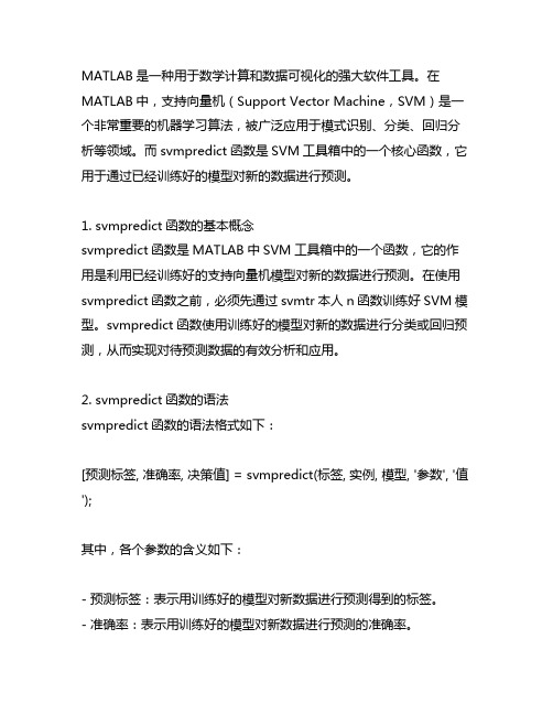
MATLAB是一种用于数学计算和数据可视化的强大软件工具。
在MATLAB中,支持向量机(Support Vector Machine,SVM)是一个非常重要的机器学习算法,被广泛应用于模式识别、分类、回归分析等领域。
而svmpredict函数是SVM工具箱中的一个核心函数,它用于通过已经训练好的模型对新的数据进行预测。
1. svmpredict函数的基本概念svmpredict函数是MATLAB中SVM工具箱中的一个函数,它的作用是利用已经训练好的支持向量机模型对新的数据进行预测。
在使用svmpredict函数之前,必须先通过svmtr本人n函数训练好SVM模型。
svmpredict函数使用训练好的模型对新的数据进行分类或回归预测,从而实现对待预测数据的有效分析和应用。
2. svmpredict函数的语法svmpredict函数的语法格式如下:[预测标签, 准确率, 决策值] = svmpredict(标签, 实例, 模型, '参数', '值');其中,各个参数的含义如下:- 预测标签:表示用训练好的模型对新数据进行预测得到的标签。
- 准确率:表示用训练好的模型对新数据进行预测的准确率。
- 决策值:表示用训练好的模型对新数据进行预测的决策值。
标签、实例和模型分别表示待预测数据的标签、特征向量和训练好的SVM模型。
参数和值表示svmpredict函数的可选参数及其取值。
3. svmpredict函数的应用svmpredict函数在实际应用中具有广泛的用途。
在图像识别领域,可以利用svmpredict函数对图像进行特征提取和分类预测;在生物信息学领域,可以利用svmpredict函数对生物数据进行分类和回归分析;在金融领域,可以利用svmpredict函数对股票或期货数据进行趋势预测等。
4. 使用示例接下来通过一个简单的示例来演示svmpredict函数的使用方法。
假设我们有一组已经训练好的SVM模型,现在需要利用这个模型对新的数据进行分类预测。
- 1、下载文档前请自行甄别文档内容的完整性,平台不提供额外的编辑、内容补充、找答案等附加服务。
- 2、"仅部分预览"的文档,不可在线预览部分如存在完整性等问题,可反馈申请退款(可完整预览的文档不适用该条件!)。
- 3、如文档侵犯您的权益,请联系客服反馈,我们会尽快为您处理(人工客服工作时间:9:00-18:30)。
%构造训练样本
n = 50;
randn('state',6);
x1 = randn(2,n); %2行N列矩阵
y1 = ones(1,n); %1*N个1
x2 = 5+randn(2,n); %2*N矩阵
y2 = -ones(1,n); %1*N个-1
figure;
plot(x1(1,:),x1(2,:),'bx',x2(1,:),x2(2,:),'k.');
%x1(1,:)为x1的第一行,x1(2,:)为x1的第二行
axis([-3 8 -3 8]);
title('C-SVC')
hold on;
X = [x1,x2]; %训练样本d*n矩阵,n为样本个数,d为特征向量个数
Y = [y1,y2]; %训练目标1*n矩阵,n为样本个数,值为+1或-1
%训练支持向量机
function svm = svmTrain(svmType,X,Y,ker,p1,p2)
options = optimset; % Options是用来控制算法的选项参数的向量
rgeScale = 'off';
options.Display = 'off';
switch svmType
case'svc_c',
C = p1;
n = length(Y);
H = (Y'*Y).*kernel(ker,X,X);
f = -ones(n,1); %f为1*n个-1,f相当于Quadprog函数中的c
A = [];
b = [];
Aeq = Y; %相当于Quadprog函数中的A1,b1
beq = 0;
lb = zeros(n,1); %相当于Quadprog函数中的LB,UB
ub = C*ones(n,1);
a0 = zeros(n,1); % a0是解的初始近似值
[a,fval,eXitflag,output,lambda] = quadprog(H,f,A,b,Aeq,beq,lb,ub,a0,options); %a是输出变量,它是问题的解
% Fval是目标函数在解a 处的值
% Exitflag>0,则程序收敛于解x
Exitflag=0,则函数的计算达到了最大次数
Exitflag<0,则问题无可行解,或程序运行失败
% Output 输出程序运行的某些信息
%Lambda 为在解a 处的值Lagrange 乘子
%支持向量机的数学表达式:
()()C
y st X X K y y W i i l
i i j i j i j l
j i i l
i i ≤≤=+-=∑∑∑===αααααα00
:,21min 11,1
(i=1 to L)
Quadprog 函数:
cx Hx x T
+2
1min
St:()
()
()
有界约束等式约束
不等式约束UB x LB b x A b Ax ≤≤=≤11
因此,H = (Y'*Y).*kernel(ker,X,X)
支持向量机的数学表达式中的最优解为
T l
),...,(***1
ααα=,∑==l
i i i i x y W 1
**α,
)2/()*(*1
*1
*∑∑==-=i y i l
i i i x W B αα
%寻找支持向量
a = svm.a;
epsilon = 1e-8;
i_sv = find(abs(a)>epsilon); %0<a<a(max)则认为x 为支持向量 plot(X(1,i_sv),X(2,i_sv),'ro');
%构造测试数本
[x1,x2] = meshgrid(-2:0.05:7,-2:0.05:7); %x1和x2都是181*181的矩阵 [rows,cols] = size(x1); %M=size(x1,1):返回x 数组的行数181
%N=size(x1,2):返回x 数组的列数181
nt = rows*cols;
Xt = [reshape(x1,1,nt);reshape(x2,1,nt)];
%reshape(x1,1,nt)是将x1转成1*(181*181)的矩阵;所以Xt 是一个2*(181*181)的矩阵
%测试输出
tmp = (a.*Y)*kernel(ker,X,X(:,i_sv)); %∑==l
i i i i x X K y a
tmp 1
*),(
b = 1./Y(i_sv)-tmp;
b = mean(b); %∑=-=l
i j i i i x x K yi y b
1
*),(α
tmp = (a.*Y)*kernel(ker,X,Xt); %∑==
l
i i i i x X K y a
tmp 1
*
),( Xt 是要进行判别
Yd = sign(tmp+b); % }),(sgn{)(1
*∑=+=l
i i i i b X x K a y x f
%分界面
Yd = reshape(Yd,rows,cols)
contour(x1,x2,Yd,[0 0],'m'); % Contour 函数:曲面的等高线图。