基于DCT变换的图像编解码matlab代码
数字图像处理 实验四dct编码

实验程序和结果:实验所使用的图像:1、利用Huffman进行JPEG图像压缩编码程序:I=imread('F\.jpg');pix(256)=struct('huidu',0.0,...%灰度值'number',0.0,...%对应像素的个数'bianma','');%对应灰度的编码[m n l]=size(I);fid=fopen('huffman.txt','w');%huffman.txt是灰度级及相应的编码表fid1=fopen('huff_compara.txt','w');%huff_compara.txt是编码表huf_bac=cell(1,l);for t=1:l%初始化结构数组for i=1:256pix(i).number=1;pix(i).huidu=i-1;%灰度级是0—255,因此是i-1pix(i).bianma='';end%统计每种灰度像素的个数记录在pix数组中for i=1:mfor j=1:nk=I(i,j,t)+1;%当前的灰度级pix(k).number=1+pix(k).number;endend%按灰度像素个数从大到小排序for i=1:255for j=i+1:256if pix(i).number<pix(j).numbertemp=pix(j);pix(j)=pix(i);pix(i)=temp;endendend%因为有的灰度值在图像中可能没有对应的像素值,所以要%找出在图像中存在像素的灰度级的个数,并保存在num中for i=256:-1:1if pix(i).number ~=0break;endendnum=i;count(t)=i;%记录每层灰度级%定义用于求解的矩阵clear huffmanhuffman(num,num)=struct('huidu',0.0,...'number',0.0,...'bianma','');huffman(num,:)=pix(1:num);%矩阵赋值for i=num-1:-1:1p=1;%算出队列中数量最少的两种灰度的像素个数的和sum=huffman(i+1,i+1).number+huffman(i+1,i).number;for j=1:i%如果当前要复制的结构体的像素个数大于sum就直接复制if huffman(i+1,p).number>sumhuffman(i,j)=huffman(i+1,p);p=p+1;else%如果当前要复制的结构体的像素个数小于或等于sum就插入和的结构体%灰度值为-1标志这个结构体的number是两种灰度像素的和huffman(i,j).huidu=-1;huffman(i,j).number=sum;sum=0;huffman(i,j+1:i)=huffman(i+1,j:i-1);break;endendend%开始给每个灰度值编码for i=1:num-1obj=0;for j=1:iif huffman(i,j).huidu==-1obj=j;break;elsehuffman(i+1,j).bianma=huffman(i,j).bianma;endendif huffman(i+1,i+1).number>huffman(i+1,i).number%说明:大概率的编0,小概率的编1,概率相等的,标号大的为1,标号小的为0 huffman(i+1,i+1).bianma=[huffman(i,obj).bianma '0'];huffman(i+1,i).bianma=[huffman(i,obj).bianma '1'];elsehuffman(i+1,i+1).bianma=[huffman(i,obj).bianma '1'];huffman(i+1,i).bianma=[huffman(i,obj).bianma '0'];endfor j=obj+1:ihuffman(i+1,j-1).bianma=huffman(i,j).bianma;endendfor k=1:count(t)huf_bac(t,k)={huffman(num,k)}; %保存endend%写出灰度编码表for t=1:lfor b=1:count(t)fprintf(fid,'%d',huf_bac{t,b}.huidu);fwrite(fid,' ');fprintf(fid,'%s',huf_bac{t,b}.bianma);fwrite(fid,' ');endfwrite(fid,'%');%先写灰度值,再写灰度级所对应的哈夫曼编码,并用将每个层级的灰度隔开end%按原图像数据,写出相应的编码,也就是将原数据用哈夫曼编码替代for t=1:lfor i=1:mfor j=1:nfor b=1:count(t)if I(i,j,t)==huf_bac{t,b}.huiduM(i,j,t)=huf_bac{t,b}.huidu;%将灰度级存入解码的矩阵fprintf(fid1,'%s',huf_bac{t,b}.bianma);fwrite(fid1,' ');%用空格将每个灰度编码隔开break;endendendfwrite(fid1,',');%用空格将每行隔开endfwrite(fid1,'%');%用%将每层灰度级代码隔开endfclose(fid);fclose(fid1);M=uint8(M);save('M')%存储解码矩阵编码结果:Huffman编码表:Huffman代码:Huffman解码程序:function huf_decode%哈夫曼编码解码load MI=imread('F:\Heat.jpg');subplot(1,2,1),imshow(I),title('原图')%读出原图subplot(1,2,2),imshow(M),title('huffman解码后的图')%读出解码后的图解码结果:2、利用行程编码进行图像压缩的MATLAB程序function yc%行程编码算法%读图I=imread('zbz.jpg');[m n l]=size(I);fid=fopen('yc.txt','w');%yc.txt是行程编码算法的灰度级及其相应的编码表%行程编码算法sum=0;for k=1:lfor i=1:mnum=0;J=[];value=I(i,1,k);for j=2:nif I(i,j,k)==valuenum=num+1;%统计相邻像素灰度级相等的个数if j==nJ=[J,num,value];endelse J=[J,num,value];%J的形式是先是灰度的个数及该灰度的值 value=I(i,j,k);num=1;endendcol(i,k)=size(J,2);%记录Y中每行行程行程编码数sum=sum+col(i,k);Y(i,1:col(i,k),k)=J;%将I中每一行的行程编码J存入Y的相应行中 endend%输出相关数据[m1,n1,l1]=size(Y);disp('原图像大小:')whos('I');disp('压缩图像大小:')whos('Y');disp('图像的压缩比:');disp(m*n*l/sum);%将编码写入yc.txt中for k=1:l1for i=1:m1for j=1:col(i,k)fprintf(fid,'%d',Y(i,j,k));fwrite(fid,' ');endendfwrite(fid,' ');endsave('Y')%存储,以便解码用save('col')fclose(fid);结果:编码代码:function yc_decode%行程编编码解码load Y %下载行程编码Yload col %下载Y中每行行程行程编码数[m,n,l]=size(Y);for k=1:lfor i=1:mp=1;for j=1:2:col(i,k)d=Y(i,j,k);%灰度值的个数for c=p:p+d-1X(i,c,k)=Y(i,j+1,k);%将d个灰度值存入X中endp=p+d;endendendI=imread('zbz.jpg');subplot(1,2,1),imshow(I),title('原图')%读出原图subplot(1,2,2),imshow(X),title('行程编码解码后的图')%读出解码后的图解码后:3、利用DCT进行图像压缩的MATLAB程序I=imread(‘rice.png’); %读入原图像;I=im2double(I); %将原图像转为双精度数据类型;T=dctmtx(8); %产生二维DCT变换矩阵B=blkproc(I,[8 8],’P1*x*P2’,T,T’); %计算二维DCT,矩阵T 及其转置T’是DCT函数P1*x*P2的参数Mask=[ 1 1 1 1 0 0 0 01 1 1 0 0 0 0 01 1 0 0 0 0 0 01 0 0 0 0 0 0 00 0 0 0 0 0 0 00 0 0 0 0 0 0 00 0 0 0 0 0 0 00 0 0 0 0 0 0 0]; %二值掩膜,用来压缩DCT系数,只留下DCT系数中左上角的10个B2=blkproc(B,[8 8],’ P1.*x.’,mask); %只保留DCT变换的10个系数I2= blkproc(B2,[8,8],’P1*x*P2’,T’,T); %逆DCT,重构图像Subplot(1,2,1);Imshow(I);title(‘原图像’); %显示原图像Subplot(1,2,2);Imshow(I2);title(‘压缩图像’);%显示压缩后的图像实验结果:。
数字图像处理及matlab实现源代码【1】
% *-*--*-*-*-*-*-*-*-*-*-*-*图像处理*-*-*-*-*-*-*-*-*-*-*-*%{% (一)图像文件的读/写A=imread('drum.jpg'); % 读入图像imshow(A); % 显示图像imwrite(A,'drum.jpg');info=imfinfo('drum.jpg') % 查询图像文件信息% 用colorbar函数将颜色条添加到坐标轴对象中RGB=imread('drum.jpg');I=rgb2gray(RGB); % 把RGB图像转换成灰度图像h=[1 2 1;0 0 0;-1 -2 -1];I2=filter2(h,I);imshow(I2,[]);colorbar('vert') % 将颜色条添加到坐标轴对象中% wrap函数将图像作为纹理进行映射A=imread('4.jpg');imshow(A);I=rgb2gray(RGB);[x,y,z]=sphere;warp(x,y,z,I); % 用warp函数将图像作为纹理进行映射%}% subimage函数实现一个图形窗口中显示多幅图像RGB=imread('drum.jpg');I=rgb2gray(RGB);subplot(1,2,1);subimage(RGB); % subimage函数实现一个图形窗口中显示多幅图像subplot(1,2,2),subimage(I);% *-*--*-*-*-*-*-*-*-*-*-*-*图像处理*-*-*-*-*-*-*-*-*-*-*-*% (二)图像处理的基本操作% ----------------图像代数运算------------------%{% imadd函数实现两幅图像的相加或给一幅图像加上一个常数% 给图像每个像素都增加亮度I=imread('4.jpg');J=imadd(I,100); % 给图像增加亮度subplot(1,2,1),imshow(I);title('原图');subplot(1,2,2),imshow(J);title('增加亮度图');%% imsubtract函数实现将一幅图像从另一个图像中减去或减去一个常数I=imread('drum.jpg');J=imsubtract(I,100); % 给图像减去亮度subplot(1,2,1),imshow(I);%% immultiply实现两幅图像的相乘或者一幅图像的亮度缩放I=imread('drum.jpg');J=immultiply(I,2); % 进行亮度缩放subplot(1,2,1),imshow(I);subplot(1,2,2),imshow(J);%% imdivide函数实现两幅图像的除法或一幅图像的亮度缩放I=imread('4.jpg');J=imdivide(I,0.5); % 图像的亮度缩放subplot(1,2,1),imshow(I);subplot(1,2,2),imshow(J);%}% ----------------图像的空间域操作------------------%{% imresize函数实现图像的缩放J=imread('4.jpg');subplot(1,2,1),imshow(J);title('原图');X1=imresize(J,0.2); % 对图像进行缩放subplot(1,2,2),imshow(X1);title('缩放图');%% imrotate函数实现图像的旋转I=imread('drum.jpg');J=imrotate(I,50,'bilinear'); % 对图像进行旋转subplot(1,2,1),imshow(I);subplot(1,2,2),imshow(J);%% imcrop函数实现图像的剪切I=imread('drum.jpg');I2=imcrop(I,[1 100 130 112]); % 对图像进行剪切subplot(1,2,1),imshow(I);subplot(1,2,2),imshow(I2);%}% ----------------特定区域处理------------------%{% roipoly函数用于选择图像中的多边形区域I=imread('4.jpg');c=[200 250 278 248 199 172];r=[21 21 75 121 121 75];BW=roipoly(I,c,r); % roipoly函数选择图像中的多边形区域subplot(1,2,1),imshow(I);subplot(1,2,2),imshow(BW);%% roicolor函数式对RGB图像和灰度图像实现按灰度或亮度值选择区域进行处理a=imread('4.jpg');subplot(2,2,1),imshow(a);I=rgb2gray(a);BW=roicolor(I,128,225); % 按灰度值选择的区域subplot(2,2,4),imshow(BW);%% ploy2mask 函数转化指定的多边形区域为二值掩模x=[63 186 54 190 63];y=[60 60 209 204 601];bw=poly2mask(x,y,256,256); % 转化指定的多边形区域为二值掩模imshow(bw);hold onplot(x,y,'r','LineWidth',2);hold off%% roifilt2函数实现区域滤波a=imread('4.jpg');I=rgb2gray(a);c=[200 250 278 248 199 172];r=[21 21 75 121 121 75];BW=roipoly(I,c,r); % roipoly函数选择图像中的多边形区域h=fspecial('unsharp');J=roifilt2(h,I,BW); % 区域滤波subplot(1,2,1),imshow(I);subplot(1,2,2),imshow(J);%% roifill函数实现对特定区域进行填充a=imread('4.jpg');I=rgb2gray(a);c=[200 250 278 248 199 172];r=[21 21 75 121 121 75];J=roifill(I,c,r); % 对特定区域进行填充subplot(1,2,1),imshow(I);subplot(1,2,2),imshow(J);%}% ----------------图像变换------------------%{% fft2 和ifft2函数分别是计算二维的快速傅里叶变换和反变换f=zeros(100,100);subplot(1,2,1);imshow(f);f(20:70,40:60)=1;subplot(1,2,2);imshow(f);F=fft2(f); % 计算二维的快速傅里叶变换F2=log(abs(F));% 对幅值对对数figure;subplot(1,2,1),imshow(F),colorbar;subplot(1,2,2),imshow(F2),colorbar;%% fftsshift 函数实现了补零操作和改变图像显示象限f=zeros(100,100);subplot(2,2,1),imshow(f);title('f')f(10:70,40:60)=1;subplot(2,2,2),imshow(f);title('f取后')F=fft2(f,256,256);subplot(2,2,3),imshow(F);title('F')F2=fftshift(F); % 实现补零操作subplot(2,2,4),imshow(F2);title('F2')figure,imshow(log(abs(F2)));title('log(|F2|)')%% dct2 函数采用基于快速傅里叶变换的算法,用于实现较大输入矩阵的离散余弦变换% idct2 函数实现图像的二维逆离散余弦变换RGB=imread('drum.jpg');I=rgb2gray(RGB);J=dct2(I); % 对I进行离散余弦变换imshow(log(abs(J))),title('对原图离散后取对数'),colorbar;J(abs(J)<10)=0;K=idct2(J); % 图像的二维逆离散余弦变换figure,imshow(I),title('原灰度图')figure,imshow(K,[0,255]);title('逆离散变换');%% dctmtx 函数用于实现较小输入矩阵的离散余弦变figure;RGB=imread('4.jpg');I=rgb2gray(RGB);subplot(3,2,1),imshow(I),title('原灰度图');I=im2double(I);subplot(3,2,2),imshow(I),title('取双精度后');T=dctmtx(8); % 离散余弦变换subplot(3,2,3),imshow(I),title('离散余弦变换后');B=blkproc(I,[8,8],'P1*x*P2',T,T');subplot(3,2,4),imshow(B),title('blkproc作用I后的B');mask=[ 1 1 1 1 0 0 0 01 1 1 0 0 0 0 01 1 0 0 0 0 0 01 0 0 0 0 0 0 00 0 0 0 0 0 0 00 0 0 0 0 0 0 00 0 0 0 0 0 0 00 0 0 0 0 0 0 0 ];B2=blkproc(B,[8,8],'P1.*x',mask);subplot(3,2,5),imshow(B2),title('blkproc作用B后的B2');I2=blkproc(B2,[8,8],'P1*x*P2',T',T);subplot(3,2,6),imshow(I2),title('blkproc作用B2后的I2');%% edge函数用于提取图像的边缘RGB=imread('4.jpg');I=rgb2gray(RGB);BW=edge(I);imshow(I);figure,imshow(BW);%% radon 函数用来计算指定方向上图像矩阵的投影RGB=imread('4.jpg');I=rgb2gray(RGB);BW=edge(I);theta=0:179;[R,XP]=radon(BW,theta); % 图像矩阵的投影figure,imagesc(theta,XP,R);colormap(hot);xlabel('\theta(degrees)');ylabel('x\prime');title('R_{\theta}(x\prime)');colorbar;%}% ----------------图像增强、分割和编码------------------%{% imhist 函数产生图像的直方图A=imread('4.jpg');B=rgb2gray(A);subplot(2,1,1),imshow(B);subplot(2,1,2),imhist(B);%% histeq 函数用于对图像的直方图均衡化A=imread('4.jpg');B=rgb2gray(A);subplot(2,1,1),imshow(B);subplot(2,1,2),imhist(B);C=histeq(B); % 对图像B进行均衡化figure;subplot(2,1,1),imshow(C);subplot(2,1,2),imhist(C);%% filter2 函数实现均值滤波a=imread('4.jpg');I=rgb2gray(a);subplot(2,2,1),imshow(I);K1=filter2(fspecial('average',3),I)/255; % 3*3的均值滤波K2=filter2(fspecial('average',5),I)/255; % 5*5的均值滤波K3=filter2(fspecial('average',7),I)/255; % 7*7的均值滤波subplot(2,2,2),imshow(K1);subplot(2,2,3),imshow(K2);subplot(2,2,4),imshow(K3);%% wiener2 函数实现Wiener(维纳)滤波a=imread('4.jpg');I=rgb2gray(a);subplot(2,2,1),imshow(I);K1=wiener2(I,[3,3]); % 3*3 wiener滤波K2=wiener2(I,[5,5]); % 5*5 wiener滤波K3=wiener2(I,[7,7]); % 7*7 wiener滤波subplot(2,2,2),imshow(K1);subplot(2,2,3),imshow(K2);subplot(2,2,4),imshow(K3);%% medfilt2 函数实现中值滤波a=imread('4.jpg');I=rgb2gray(a);subplot(2,2,1),imshow(I);K1=medfilt2(I,[3,3]); % 3*3 中值滤波K2=medfilt2(I,[5,5]); % 5*5 中值滤波K3=medfilt2(I,[7,7]); % 7*7 中值滤波subplot(2,2,2),imshow(K1);subplot(2,2,3),imshow(K2);subplot(2,2,4),imshow(K3);%}% ----------------图像模糊及复原------------------%{% deconvwnr 函数:使用维纳滤波器I=imread('qier.jpg');imshow(I);% 对图像进行模糊处理LEN=31;THETA=11;PSF1=fspecial('motion',LEN,THETA); % 运动模糊PSF2=fspecial('gaussian',10,5); % 高斯模糊Blurred1=imfilter(I,PSF1,'circular','conv'); % 得到运动模糊图像Blurred2=imfilter(I,PSF2,'conv'); % 得到高斯噪声模糊图像figure;subplot(1,2,1);imshow(Blurred1);title('Blurred1--"motion"'); subplot(1,2,2);imshow(Blurred2);title('Blurred2--"gaussian"');% 对模糊图像加噪声V=0.002;BlurredNoisy1=imnoise(Blurred1,'gaussian',0,V); % 加高斯噪声BlurredNoisy2=imnoise(Blurred2,'gaussian',0,V); % 加高斯噪声figure;subplot(1,2,1);imshow(BlurredNoisy1);title('BlurredNoisy1'); subplot(1,2,2);imshow(BlurredNoisy2);title('BlurredNoisy2');% 进行维纳滤波wnr1=deconvwnr(Blurred1,PSF1); % 维纳滤波wnr2=deconvwnr(Blurred2,PSF2); % 维纳滤波figure;subplot(1,2,1);imshow(wnr1);title('Restored1,True PSF'); subplot(1,2,2);imshow(wnr2);title('Restored2,True PSF');%% deconvreg函数:使用约束最小二乘滤波器I=imread('qier.jpg');imshow(I);% 对图像进行模糊处理LEN=31;THETA=11;PSF1=fspecial('motion',LEN,THETA); % 运动模糊PSF2=fspecial('gaussian',10,5); % 高斯模糊Blurred1=imfilter(I,PSF1,'circular','conv'); % 得到运动模糊图像Blurred2=imfilter(I,PSF2,'conv'); % 得到高斯噪声模糊图像figure;subplot(1,2,1);imshow(Blurred1);title('Blurred1--"motion"');subplot(1,2,2);imshow(Blurred2);title('Blurred2--"gaussian"');% 对模糊图像加噪声V=0.002;BlurredNoisy1=imnoise(Blurred1,'gaussian',0,V); % 加高斯噪声BlurredNoisy2=imnoise(Blurred2,'gaussian',0,V); % 加高斯噪声figure;subplot(1,2,1);imshow(BlurredNoisy1);title('BlurredNoisy1');subplot(1,2,2);imshow(BlurredNoisy2);title('BlurredNoisy2');NP=V*prod(size(I));reg1=deconvreg(BlurredNoisy1,PSF1,NP); % 约束最小二乘滤波reg2=deconvreg(BlurredNoisy2,PSF2,NP); % 约束最小二乘滤波figure;subplot(1,2,1);imshow(reg1);title('Restored1 with NP');subplot(1,2,2);imshow(reg2);title('Restored2 with NP');%% deconvlucy函数:使用Lucy-Richardson滤波器I=imread('qier.jpg');imshow(I);% 对图像进行模糊处理LEN=31;THETA=11;PSF1=fspecial('motion',LEN,THETA); % 运动模糊PSF2=fspecial('gaussian',10,5); % 高斯模糊Blurred1=imfilter(I,PSF1,'circular','conv'); % 得到运动模糊图像Blurred2=imfilter(I,PSF2,'conv'); % 得到高斯噪声模糊图像figure;subplot(1,2,1);imshow(Blurred1);title('Blurred1--"motion"');subplot(1,2,2);imshow(Blurred2);title('Blurred2--"gaussian"');% 对模糊图像加噪声V=0.002;BlurredNoisy1=imnoise(Blurred1,'gaussian',0,V); % 加高斯噪声BlurredNoisy2=imnoise(Blurred2,'gaussian',0,V); % 加高斯噪声figure;subplot(1,2,1);imshow(BlurredNoisy1);title('BlurredNoisy1');subplot(1,2,2);imshow(BlurredNoisy2);title('BlurredNoisy2');luc1=deconvlucy(BlurredNoisy1,PSF1,5); % 使用Lucy-Richardson滤波luc2=deconvlucy(BlurredNoisy1,PSF1,15); % 使用Lucy-Richardson滤波figure;subplot(1,2,1);imshow(luc1);title('Restored Image,NUMIT=5'); subplot(1,2,2);imshow(luc2);title('Restored Image,NUMIT=15');%}% deconvblind 函数:使用盲卷积算法a=imread('4.jpg');I=rgb2gray(a);figure;imshow(I);title('Original Image');PSF=fspecial('motion',13,45); % 运动模糊figure;imshow(PSF);Blurred=imfilter(I,PSF,'circ','conv'); % 得到运动模糊图像figure;imshow(Blurred);title('Blurred Image');INITPSF=ones(size(PSF));[J,P]=deconvblind(Blurred,INITPSF,30); % 使用盲卷积figure;imshow(J);figure;imshow(P,[],'notruesize');% *-*--*-*-*-*-*-*-*-*-*-*-*图像处理*-*-*-*-*-*-*-*-*-*-*-* %{% 对图像进行减采样a=imread('lena.jpg');%subplot(1,4,1);figure;imshow(a);title('原图');b=rgb2gray(a);%subplot(1,4,2);figure;imshow(b);title('原图的灰度图');[wid,hei]=size(b);%---4倍减采样----quartimg=zeros(wid/2+1,hei/2+1);i1=1;j1=1;for i=1:2:widfor j=1:2:heiquartimg(i1,j1)=b(i,j);j1=j1+1;endi1=i1+1;j1=1;end%subplot(1,4,3);figure;imshow(uint8(quartimg));title('4倍减采样')% ---16倍减采样---quanrtimg=zeros(wid/4+1,hei/4+1);i1=1;j1=1;for i=1:4:widfor j=1:4:heiquanrtimg(i1,j1)=b(i,j);j1=j1+1;endi1=i1+1;j1=1;end%subplot(1,4,4);.figure;imshow(uint8(quanrtimg));title('16倍减采样');%}% 图像类型% 将图像转换为256级灰度图像,64级灰度图像,32级灰度图像,8级灰度图像,2级灰度图像a=imread('4.jpg');%figure;subplot(2,3,1);imshow(a);title('原图');b=rgb2gray(a); % 这是256灰度级的图像%figure;subplot(2,3,2);imshow(b);title('原图的灰度图像');[wid,hei]=size(b);img64=zeros(wid,hei);img32=zeros(wid,hei);img8=zeros(wid,hei);img2=zeros(wid,hei);for i=1:widfor j=j:heiimg64(i,j)=floor(b(i,j)/4); % 转化为64灰度级endend%figure;subplot(2,3,3);imshow(uint8(img64),[0,63]);title('64级灰度图像');for i=1:widfor j=1:heiimg32(i,j)=floor(b(i,j)/8);% 转化为32灰度级endend%figure;subplot(2,3,4);imshow(uint8(img32),[0,31]);title('32级灰度图像');for i=1:widfor j=1:heiimg8(i,j)=floor(b(i,j)/32);% 转化为8灰度级endend%figure;subplot(2,3,5);imshow(uint8(img8),[0,7]);title('8级灰度图像');for i=1:widfor j=1:heiimg2(i,j)=floor(b(i,j)/128);% 转化为2灰度级endend%figure;subplot(2,3,6);imshow(uint8(img2),[0,1]);title('2级灰度图像');% *-*--*-*-*-*-*-*-*-*-*-*-*图像处理*-*-*-*-*-*-*-*-*-*-*-* %{% ------------------ 图像的点运算------------------I=imread('lena.jpg');figure;subplot(1,3,1);imshow(I);title('原图的灰度图');J=imadjust(I,[0.3;0.6],[0.1;0.9]); % 设置灰度变换的范围subplot(1,3,2);imshow(J);title('线性扩展');I1=double(I); % 将图像转换为double类型I2=I1/255; % 归一化此图像C=2; % 非线性扩展函数的参数K=C*log(1+I2); % 对图像的对数变换subplot(1,3,3);imshow(K);title('非线性扩展');M=255-I;figure;subplot(1,3,1);imshow(M);title('灰度倒置');N1=im2bw(I,0.4); % 将此图像二值化,阈值为0.4N2=im2bw(I,0.7); % 将此图像二值化,阈值为0.7 subplot(1,3,2);imshow(N1);title('二值化阈值0.4');subplot(1,3,3);imshow(N2);title('二值化阈值0.7');%}%{% ------------------ 图像的代数运算------------------% 将两幅图像进行加法运算I=imread('lena.jpg');I=rgb2gray(I);J=imread('rice.png');% 以下把两幅图转化为大小一样for i=1:size(I)for j=size(J):size(I)J(i,j)=0;endendI=im2double(I); % 将图像转化为double型J=im2double(J);% imshow(I);figure;imshow(J);K=I+0.3*J; % 将两幅图像相加subplot(1,3,1);imshow(I);title('人物图');subplot(1,3,2);imshow(J);title('背景图');subplot(1,3,3);imshow(K);title('相加后的图');imwrite(K,'i_lena1.jpg');%%% 将两幅图像做减运算,分离背景与原图A=imread('i_lena1.jpg');B=imread('rice.png');% 以下把两幅图转化为大小一样for i=1:size(A)for j=size(B):size(A)B(i,j)=0;endendC=A-0.3*B;a=imread('lena.jpg');subplot(2,2,1);imshow(a);title('原图图');subplot(2,2,2);imshow(A);title('混合图');subplot(2,2,3);imshow(B);title('背景图');subplot(2,2,4);imshow(C);title('分离后的图');%% 设置掩模,需要保留下来的区域,掩模图像的值为1,否则为0 A=imread('drum.jpg');A=rgb2gray(A);A=im2double(A);sizeA=size(A);subplot(1,2,1);imshow(A);title('原图');B=zeros(sizeA(1),sizeA(2)); % 设置模板B(100:400,100:500)=1;K=A.*B; % 两幅图像相乘subplot(1,2,2);imshow(K);title('局部图');%}%{% ------------------ 图像的缩放------------------A=imread('drum.jpg');B1=imresize(A,1.5); % 比例放大1.5杯,默认采用的是最近邻法进行线性插值B2=imresize(A,[420 384]); % 非比例放大到420:384C1=imresize(A,0.7); % 比例缩小0.7倍C2=imresize(A,[150 180]); % 非比例缩小到150:180figure;imshow(B1);title('比例放大图');figure;imshow(B2);title('非比例放大图');figure;imshow(C1);title('比例缩小图');figure;imshow(C2);title('非比例缩小图');% 检测非比例缩放得到的图片是否能还原到原图a=size(A)d=imresize(C2,[a(1),a(2)]);figure;imshow(d);%}% ------------------ 图像的旋转------------------I=imread('drum.jpg');J=imrotate(I,45); % 图像进行逆时针旋转,默认采用最近邻插值法进行插值处理K=imrotate(I,90); % 默认旋转出界的部分不被截出subplot(1,3,1);imshow(I);subplot(1,3,2);imshow(J);subplot(1,3,3);imshow(K);% 检测旋转后的图像是否失真P=imrotate(K,270);figure;imshow(P);。
基于局部方差和DCT变换的混合分形图像编码算法

Ab ta t Th r c a g o r s i n i r mii g t c n l g .I o t a twih o h r o r s i n me h d ,fa — sr c e fa t l ma ec mp e so sa p o s n e h o o y n c n r s t t e mp e so t o s r c i c
摘 要 分形 图像编码技术是一种很有发展前途 的新型 图像 编码技 术, 相对 于已有的其它 图像编码算 法, 分形图像 编
码算 法能够在取得 高压 缩率的前提 下, 较好 地保持解码 图像的质量 。本文根据 图像 内部的 图像子块特征 , 出了一种 提 基 于局部 方差和 D T变换的混合分形 图像编码算法 , 算法在 大幅提 高分形编码 速度 的同时 , C 该 很好 地改善 了解码 图
t1i g o p eso a b an g o e o ig q aiywih hg p eso ai. Thsp p rp o o e o ie a ma ec m r sinc n o ti o d d c dn u l t ih c m r sin rt t o i a e r p s sac mbn d
f a t l ma e c mp e s n a g rt m a e n DCT n a i n e n h o e l o i m b an o d q a iy o h r ca i g o r s i lo i o h bsdo a d v ra c ,a d t e n v lag rt h o t i s g o u l ft e t d c d d i g s a d n e c e s tme t a h a ei e f a t l l o ih e o e ma e n e d mu h l s i h n t e b s l r c a g rt m. Ex e i n a e u t h w h t t e p o n a pr me t lr s l s o t a h r — s p s dag r h a ne c l n ef r n e o e l o im h s a x el tp ro ma c . t e Ke wo d Fr c a ma e c mp e so ,Va in e y rs a t 1i g o r s i n r c ,DCT r n f r a i n a t a so m t o
基于DCT的JPEG图像压缩编码算法的MATLAB实现
维普资讯
第1 第 1 5卷 期
20 年 3 02 - 月
J u a fZ i gWa l U iesy o r l } a ni nv ri n o n t
浙 江万里学院学报
V
b , o】
Ma 2 0 r 02
文章 编号 :6 1 2o2o ]l 0 2 —0. 17 —25 io 2o 一 08 4 -
和解 压过程 .
12 结 合 M T  ̄ 53仿 真对上 述算法 的几点 解释 . A LB. 12 1 离散 余 弦 变挟 ( c ) D r 定义
二维 D T的解 析式定 义 可 以由下式表示 : C
F f= (yF, 等 ( ) ( )N ) ( ) c o , 0 ,,O o s
D T系数值 , 中 1 数 值是 直 流 ( C 系数 , 8×8空域 图像 子块 的平 均值 , 余 的 6 C 其 个 D) 即 其 3个 是交 流 ( c 系 A ) 数, 接下 来对 D T系数进 行量 化 , 将变 换得到 的量 比的 D T系数进 行编码 和传 送 , 成压 缩后 的图像 格 C 最后 C 形
二维 D T反变换 (D T 解析 式定 义可 以表示 为 : C IC )
几 =m, 啬 击 o ) +
+ m cs o
c o s
os o
+ os 等 m.o ) c
matlab实验,图像变换域分析(dct变换和小波变换)
实验一 图像DCT 变换一、实验目的1.了解DCT 处理图像的基本知识;2.掌握用matlab 将对图像进行DCT 变换。
二、实验内容1.对图像进行DCT 处理;2.显示变换后的图像的三维的频谱; 3.对matlab 代码进行一定的文字说明;三、实验原理离散余弦变换(Discrete Cosine Transform ,DCT )是一种实数域变换,其变换核为实数余弦函数。
对一幅图像进行离散余弦变换后,许多有关图像的重要可视信息都集中在DCT 变换的一小部分系数中。
因此,离散余弦变换(DCT )是有损图像压缩JPEG 的核心,同时也是所谓“变换域信息隐藏算法”的主要“变换域(DCT 域)”之一。
因为图像处理运用二维离散余弦变换,所以直接介绍二维DCT 变换。
一个矩阵的二维DCT 定义如下:首先将输入图像分解为8*8或16*16块,然后再对每个图像块进行二维DCT 变换,接着再对DCT 系数进行量化、编码和传输;接收者通过对量化的DCT 系数进行解码,并对每个图像块进行的二维DCT 反变换。
最后将操作完成后所有的块拼接起来构成一幅单一的图像。
对于一般的图像而言,大多数DCT 系数值都接近于0,所以去掉这些系数不会对重建图像的质量产生较大影响。
因此,利用DCT 进行图像压缩确实可以节约大量的存储空间。
在实验中,先将输入的原始图像分为8*8块,然后再对每个块进行二维DCT 变换。
MATLAB 图像处理上具箱中提供的二维DCT 变换及DCT 反变换函数如下。
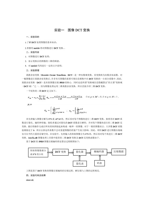
基于DCT 的JPEG 图像压缩编码理论算法过程框图如下:上图是基于DCT 变换的图像压缩编码的压缩过程,解压缩与上图的过程相反。
四、实验代码及结果close all;原始图像数据分成8*8的小块DCT 变换 量化器量化表熵编码器 码表压缩数据I=imread('222.jpg'); %读入原图像文件I=rgb2gray(I);%将原图像转换成灰色图像I1=dct2(I);%对原图像进行二维DCT变换fs=fftshift(I1);%将直流分量移到频谱中心subplot(121);imshow(I);title('灰色图像');%显示灰色图像subplot(122);imshow(log(abs(I1)),[]),colorbar;title('图像经DCT变换后能量分布情况') %显示经过dct变换后能量分布;figure(2);mesh(fs);title('三维频谱');%显示三维频谱五、实验结果分析图像经DCT变换后能量主要分布在左上角,右下角能量分布较低。
基于二维DCT的图像压缩编码及其实现
基于二维DCT的图像压缩编码及其实现作者:李春霞来源:《现代电子技术》2008年第16期摘要:DCT变换是图像压缩的一项重要技术,如何准确、快速进行图像压缩一直是国内外研究的热点。
主要介绍基于DCT变换的图像压缩编码算法,给出具体的实现方法和步骤,并用Matlab进行了算法仿真。
实验结果表明,该算法实现简单,在很大压缩范围内,都能得到很好的重建图像质量,满足不同场合要求不同图像质量的实际需要。
这里利用Matlab做仿真实验,方法简单、速度快且误差小,大大提高了图像压缩的效率和精度。
关键词:图像压缩;DCT变换;Matlab仿真;峰值信噪比中图分类号:TP391 文献标识码:B 文章编号:1004373X(2008)1615703Image Compression Coding and Implementation Based on 2DDCTLI Chunxia(College of Electric and Information Engineering,Shaanxi University of Science & Technology,Xi′an,710021,China)Abstract:The DCT transform is an important technique in the field of image compression.How to compress the image accurately and fast has been a research focus both at home and abroad all the time.This paper mainly introduces the algorithm of the image compress coding based on DCT,and shows details of realization.Then the algorithm is simulated by Matlab.Simulation experiments show that the algorithm is simple to realize.The reconstructed images are of good quality satisfying the demands of different image quality on various occasions under the circumstances of very large compression range.The innovation spot of this paper is that the method doing experiments with Matlab is simple,rapid and with little error.It can improve the efficiency and precision of the image compression greatly.Keywords:image compression;DCT transform;Matlab simulation;peak signal to noise ratio在信息世界迅猛发展的今天,图像传输已成为一项重要内容,而传输信息量的大小是影响传输速度的重要因素之一。
javadct_DCT(离散余弦变换)算法原理和源码

javadct_DCT(离散余弦变换)算法原理和源码离散余弦变换(Discrete Cosine Transform,简称DCT)是一种常用的信号处理技术,广泛应用于图像和音频压缩领域。
DCT将输入的离散信号转换为一组系数,这些系数代表了信号的频域特征。
在压缩领域中,DCT可将信号从时域转换为频域,通过舍弃一些高频系数实现信号的压缩。
DCT算法的原理基于傅里叶变换(Fourier Transform)的思想,将时域信号转换为频域信号。
然而,与傅里叶变换相比,DCT更适合处理实数信号,因为它只使用实数运算,而不需要复数运算。
DCT算法的一般步骤如下:1.将输入的离散信号分为若干个块,每个块包含N个采样点。
2.对每个块进行预处理,例如减去均值。
3.对每个块进行DCT变换。
4.根据需要舍弃一些高频系数。
5.对经过舍弃的系数进行逆DCT变换,恢复原始信号。
下面是一个简单的离散余弦变换的Python实现:```pythonimport numpy as npdef dct_transform(signal):N = len(signal)dct_coef = np.zeros(N)for k in range(N):sum = 0for n in range(N):sum += signal[n] * np.cos((np.pi/N)*(n+0.5)*k)dct_coef[k] = sumreturn dct_coefdef idct_transform(dct_coef):N = len(dct_coef)signal = np.zeros(N)for n in range(N):sum = 0for k in range(N):sum += dct_coef[k] * np.cos((np.pi/N)*(n+0.5)*k)signal[n] = sum / Nreturn signal```以上是一个简单的DCT变换和逆变换的实现,其中`dct_transform`函数接受输入信号并返回DCT系数,`idct_transform`函数接受DCT系数并返回恢复的原始信号。
MATLAB中的信号编码与解码技巧
MATLAB中的信号编码与解码技巧引言现代通信系统中,信号编码和解码是关键技术,它们在数据传输和存储中扮演着至关重要的角色。
MATLAB作为一种强大的数学计算软件和编程环境,提供了丰富的功能和工具,用于信号处理和通信系统建模。
本文将探讨MATLAB中的一些常见信号编码和解码技巧,以提供读者对这一主题的深入理解。
一、数字信号编码1. PCM编码脉冲编码调制(PCM)是一种常用的数字信号编码技术,在语音和音频传输中广泛应用。
MATLAB提供了丰富的函数,可以帮助我们实现PCM编码。
例如,使用`audioread`函数可以读取音频文件,并使用`pcmenco`函数进行PCM编码。
2. Huffman编码霍夫曼编码是一种无损数据压缩算法,可以根据数据的统计特性进行代码设计。
在MATLAB中,`huffmandict`函数可用于生成霍夫曼编码字典,`huffmanenco`函数用于对数据进行编码,`huffmandeco`函数用于解码。
二、模拟信号编码1. AM编码幅度调制(AM)是一种传统的模拟信号编码技术,常用于广播和无线电通信。
在MATLAB中,我们可以使用`ammod`函数实现AM编码,并使用`amdemod`函数进行解调。
2. FM编码频率调制(FM)是另一种常见的模拟信号编码技术,广泛应用于音频和视频传输。
在MATLAB中,`fmmod`函数可用于FM编码,`fmdemod`函数可用于解调。
三、数字信号解码1. PCM解码PCM编码的逆过程是PCM解码,MATLAB中的`pcmdeco`函数可用于解码PCM信号并恢复原始信号。
2. Huffman解码通过使用霍夫曼编码表,我们可以对霍夫曼编码进行解码。
在MATLAB中,`huffmandeco`函数可用于解码数据,并使用`huffmanenco`函数所生成的编码字典。
四、应用实例:数字音频编码数字音频编码是一个实际应用领域,通过对音频信号进行编码和解码,可以实现音频数据的压缩和传输。
- 1、下载文档前请自行甄别文档内容的完整性,平台不提供额外的编辑、内容补充、找答案等附加服务。
- 2、"仅部分预览"的文档,不可在线预览部分如存在完整性等问题,可反馈申请退款(可完整预览的文档不适用该条件!)。
- 3、如文档侵犯您的权益,请联系客服反馈,我们会尽快为您处理(人工客服工作时间:9:00-18:30)。
///////////////////////////////////////////////////////////// /////////////////////////////////////////// 基于块的变换编码//读入灰度图像数据,完成8*8像素块余弦变换并进行DCT系数矩阵量化,把得到的量化矩阵游程编码///////////////////////////////////////////////////////////// /////////////////////////////////////////#include<stdio.h>#include<iostream>#include<iomanip>#include<stdlib.h>#include<fstream>#include<math.h>#define PI 3.1415926#define WIDTH 256#define HEIGHT 256using namespace std;double arr[WIDTH][HEIGHT]={0}; //自定义数组保存文件二进制数据double dct2[8][8]={100}; //自定义数组保存待变换8*8像素块二进制数据int x(14),y(22); //任意设定开始选定数据坐标void DCT(int,int,double dct2[8][8]); //余弦变换算法函实现数double CuCv(int); //中间函数C(u),C(v) void Quant(double dct2[8][8]); //均匀量化函数void Run_level(double dct2[8][8]); //游程编码函数//*********************************************************** ********************************************void main(){char ch;int data[8][8]={0};FILE *fp = NULL; //创建文件指针并初始化//----------------------------------------------------------以二进制只读形式打开待处理IMG文件fp = fopen("LENA256.IMG","rb");if(fp == NULL)//如果失败了{printf("Buffer error! Program terminated!!\n\n");}ofstream outfile("源文件二进制数据.txt"); //建立文件char buf[24];int count = 0;//----------------------------------------------------------将读入文件的数据保存在自定义数组中for(int i (0);i<WIDTH;i++){for(int j(0);j<HEIGHT;j++){int c=fgetc(fp);arr[i][j] = c;}}fclose(fp); //关闭文件cout<<"256*256选定8*8像素块开始坐标:"<<endl<<x<<endl <<y<<endl;//----------------------------------------------------------选定8*8像素块,并保存数据到文本文件中for(int i(x);i<x+8;i++){for(int j(y);j<y+8;j++){outfile <<setw(3)<< arr[i][j] <<" ";}outfile<<endl;}outfile.close();DCT(x,y,dct2); //余弦变换Quant(dct2); //均匀量化for(int i = 0;i < 8 ;i++) //变换结果输出到文本文件中{for(int j = 0;j < 8;j++){cout<< dct2[i][j] <<" ";}}cout<<endl<<endl;Run_level(dct2);//zig-zag游程编码system("pause");}//*********************************************************** ********************************************void DCT(int m,int n,double dct2[8][8]) //余弦变换算法实现函数{for(int u(0);u<8;u++){for(int v(0);v<8;v++){double sum=0;for(int i(0);i<8;i++){for(int j(0);j<8;j++){sum=sum+(arr[m+i][n+j]*cos((2*i+1)*u*PI/16)*cos((2*j+1)*v* PI/16));}}double temp=CuCv(u)*CuCv(v);dct2[u][v]=int(temp*sum/4+0.5); //余弦变换后的值,四舍五入取整}}ofstream outfile2("余弦变换取整后数据.txt");for(int i = 0;i < 8 ;i++) //变换结果输出到文本文件中{for(int j = 0;j < 8;j++){outfile2 <<setw(3)<< dct2[i][j] <<" ";}outfile2<<endl; //得到DCT系数矩阵}outfile2.close();}//*********************************************************** ********************************************double CuCv(int a) //中间函数C(u),C(v){if(a==0){return 1/pow(2,0.5);}else{return 1;}}//*********************************************************** ********************************************void Quant(double dct2[8][8]) //均匀量化函数{int QS[8][8]={ //构建均匀量化矩阵(亮度)16,11,10,16,24,40,51,61,12,12,14,19,26,58,60,55,14,13,16,24,40,57,69,56,14,17,22,29,51,87,80,62,18,22,37,56,68,109,103,77,24,35,55,64,81,104,113,92,49,64,78,87,103,121,120,101,72,92,95,98,112,100,103,99};for(int i(0);i<8;i++){for(int j(0);j<8;j++){dct2[i][j]=int(double(dct2[i][j])/QS[i][j]+0.5);}}ofstream outfile3("均匀量化后数据.txt");for(int i = 0;i < 8 ;i++) //变换结果输出到文本文件中{for(int j = 0;j < 8;j++){outfile3 <<setw(3)<< dct2[i][j] <<" ";}outfile3<<endl; //得到DCT系数矩阵}outfile3.close();}//*********************************************************** ********************************************void Run_level(double dct2[8][8]) //游程编码函数{int k(0),a[8][8]={0};int i(0),j(0),s(0); //i=行----j=列----s=总行/列数int dir(0); //扫描方向,0:右方,1:左下,2:下方,3:右上ofstream outfile4("游程符号.txt");while(s<8*8){a[i][j]=dct2[i][j]; //初始化zig-zag扫描位置int temp0=i,temp1=j;switch(dir) //下一个扫描位置{case 0:j++; //行进方向if(i==0)dir=1;if(i==7)dir=3;break;case 1:i++;j--;if(i==7)dir=0;else if(j==0)dir=2;break;case 2:i++;if(j==0) dir=3; if(j==7) dir=1; break;case 3:i--;j++;if(j==7)dir=2;else if(i==0)dir=0;break;default:break;}if(a[temp0][temp1]!=dct2[i][j]){ //输出游程符号到文件if(a[temp0][temp1]!=0){if(k!=0) k++;outfile4<<"("<<k<<","<<a[temp0][temp1]<<") ";k=0;}}else k++;s++;}outfile4.close();}。