支持向量机的matlab代码
支持向量机(SVM)、支持向量机回归(SVR):原理简述及其MATLAB实例
支持向量机(SVM)、支持向量机回归(SVR):原理简述及其MATLAB实例一、基础知识1、关于拉格朗日乘子法和KKT条件1)关于拉格朗日乘子法2)关于KKT条件2、范数1)向量的范数2)矩阵的范数3)L0、L1与L2范数、核范数二、SVM概述1、简介2、SVM算法原理1)线性支持向量机2)非线性支持向量机二、SVR:SVM的改进、解决回归拟合问题三、多分类的SVM1. one-against-all2. one-against-one四、QP(二次规划)求解五、SVM的MATLAB实现:Libsvm1、Libsvm工具箱使用说明2、重要函数:3、示例支持向量机(SVM):原理及其MATLAB实例一、基础知识1、关于拉格朗日乘子法和KKT条件1)关于拉格朗日乘子法首先来了解拉格朗日乘子法,为什么需要拉格朗日乘子法呢?记住,有需要拉格朗日乘子法的地方,必然是一个组合优化问题。
那么带约束的优化问题很好说,就比如说下面这个:这是一个带等式约束的优化问题,有目标值,有约束条件。
那么你可以想想,假设没有约束条件这个问题是怎么求解的呢?是不是直接 f 对各个 x 求导等于 0,解 x 就可以了,可以看到没有约束的话,求导为0,那么各个x均为0吧,这样f=0了,最小。
但是x都为0不满足约束条件呀,那么问题就来了。
有了约束不能直接求导,那么如果把约束去掉不就可以了吗?怎么去掉呢?这才需要拉格朗日方法。
既然是等式约束,那么我们把这个约束乘一个系数加到目标函数中去,这样就相当于既考虑了原目标函数,也考虑了约束条件。
现在这个优化目标函数就没有约束条件了吧,既然如此,求法就简单了,分别对x求导等于0,如下:把它在带到约束条件中去,可以看到,2个变量两个等式,可以求解,最终可以得到,这样再带回去求x就可以了。
那么一个带等式约束的优化问题就通过拉格朗日乘子法完美的解决了。
更高一层的,带有不等式的约束问题怎么办?那么就需要用更一般化的拉格朗日乘子法,即KKT条件,来解决这种问题了。
matlab的svmrfe函数

一、介绍MATLAB是一种流行的技术计算软件,广泛应用于工程、科学和其他领域。
在MATLAB的工具箱中,包含了许多函数和工具,可以帮助用户解决各种问题。
其中,SVMRFE函数是MATLAB中的一个重要功能,用于支持向量机分类问题中的特征选择。
二、SVMRFE函数的作用SVMRFE函数的全称为Support Vector Machines Recursive Feature Elimination,它的作用是利用支持向量机进行特征选择。
在机器学习和模式识别领域,特征选择是一项重要的任务,通过选择最重要的特征,可以提高分类器的性能,并且减少计算和存储的开销。
特征选择问题在实际应用中经常遇到,例如在生物信息学中,选择基因表达数据中最相关的基因;在图像处理中,选择最相关的像素特征。
SVMRFE函数可以自动化地解决这些问题,帮助用户找到最佳的特征子集。
三、使用SVMRFE函数使用SVMRFE函数,用户需要准备好特征矩阵X和目标变量y,其中X是大小为m×n的矩阵,表示m个样本的n个特征;y是大小为m×1的向量,表示m个样本的类别标签。
用户还需要设置支持向量机的参数,如惩罚参数C和核函数类型等。
接下来,用户可以调用SVMRFE函数,设置特征选择的方法、评价指标以及其他参数。
SVMRFE函数将自动进行特征选择,并返回最佳的特征子集,以及相应的评价指标。
用户可以根据返回的结果,进行后续的分类器训练和预测。
四、SVMRFE函数的优点SVMRFE函数具有以下几个优点:1. 自动化:SVMRFE函数可以自动选择最佳的特征子集,减少了用户手工试验的时间和精力。
2. 高性能:SVMRFE函数采用支持向量机作为分类器,具有较高的分类精度和泛化能力。
3. 灵活性:SVMRFE函数支持多种特征选择方法和评价指标,用户可以根据自己的需求进行灵活调整。
五、SVMRFE函数的示例以下是一个简单的示例,演示了如何使用SVMRFE函数进行特征选择:```matlab准备数据load fisheririsX = meas;y = species;设置参数opts.method = 'rfe';opts.nf = 2;调用SVMRFE函数[selected, evals] = svmrfe(X, y, opts);```在这个示例中,我们使用了鸢尾花数据集,设置了特征选择的方法为递归特征消除(RFE),并且要选择2个特征。
matlab中fitcsvm函数用法
matlab中fitcsvm函数用法MATLAB中的fitcsvm函数是支持向量机(Support Vector Machine, SVM)分类器的一个功能强大的实现。
SVM是一种强大的机器学习算法,可用于解决各种分类问题。
在本文中,我们将详细介绍fitcsvm函数的用法,并逐步回答所有可能的问题。
本文将以中括号为主题,详细解释如何使用fitcsvm函数进行分类任务。
一、引言fitcsvm函数是MATLAB中实现SVM分类器的一个重要工具。
SVM是一种二分类器,它通过最大化两个类别之间的间隔来找到一个最优的超平面。
通过找到这个超平面,SVM可以在新的未标记数据上进行分类。
二、fitcsvm函数的语法fitcsvm函数有很多输入和输出参数。
下面是fitcsvm函数的一般语法:SVMModel = fitcsvm(X, Y)SVMModel = fitcsvm(X, Y, 'Name', value)其中,X是一个包含训练数据的矩阵,每一行代表一个样本,每一列代表一个特征。
Y是一个包含训练数据的标签向量,指示每个样本的类别。
三、输入参数的解释fitcsvm函数除了必需的X和Y参数外,还有其他参数可以调整以获得更好的分类结果。
下面是一些常用的参数及其解释:1. 'BoxConstraint':表示SVM的惩罚因子,用于控制错误分类的重要性。
值越大,对错误分类的惩罚越严重。
2. 'KernelFunction':表示SVM使用的核函数。
常见的核函数有'linear'(线性核函数),'gaussian'(高斯核函数),'polynomial'(多项式核函数)等。
3. 'KernelScale':表示SVM的核函数标准差。
对于高斯核函数和多项式核函数,该参数可以控制决策边界的平滑程度。
4. 'Standardize':表示是否对输入数据进行标准化。
30个智能算法matlab代码
30个智能算法matlab代码以下是30个使用MATLAB编写的智能算法的示例代码: 1. 线性回归算法:matlab.x = [1, 2, 3, 4, 5];y = [2, 4, 6, 8, 10];coefficients = polyfit(x, y, 1);predicted_y = polyval(coefficients, x);2. 逻辑回归算法:matlab.x = [1, 2, 3, 4, 5];y = [0, 0, 1, 1, 1];model = fitglm(x, y, 'Distribution', 'binomial'); predicted_y = predict(model, x);3. 支持向量机算法:matlab.x = [1, 2, 3, 4, 5; 1, 2, 2, 3, 3];y = [1, 1, -1, -1, -1];model = fitcsvm(x', y');predicted_y = predict(model, x');4. 决策树算法:matlab.x = [1, 2, 3, 4, 5; 1, 2, 2, 3, 3]; y = [0, 0, 1, 1, 1];model = fitctree(x', y');predicted_y = predict(model, x');5. 随机森林算法:matlab.x = [1, 2, 3, 4, 5; 1, 2, 2, 3, 3]; y = [0, 0, 1, 1, 1];model = TreeBagger(50, x', y');predicted_y = predict(model, x');6. K均值聚类算法:matlab.x = [1, 2, 3, 10, 11, 12]; y = [1, 2, 3, 10, 11, 12]; data = [x', y'];idx = kmeans(data, 2);7. DBSCAN聚类算法:matlab.x = [1, 2, 3, 10, 11, 12]; y = [1, 2, 3, 10, 11, 12]; data = [x', y'];epsilon = 2;minPts = 2;[idx, corePoints] = dbscan(data, epsilon, minPts);8. 神经网络算法:matlab.x = [1, 2, 3, 4, 5];y = [0, 0, 1, 1, 1];net = feedforwardnet(10);net = train(net, x', y');predicted_y = net(x');9. 遗传算法:matlab.fitnessFunction = @(x) x^2 4x + 4;nvars = 1;lb = 0;ub = 5;options = gaoptimset('PlotFcns', @gaplotbestf);[x, fval] = ga(fitnessFunction, nvars, [], [], [], [], lb, ub, [], options);10. 粒子群优化算法:matlab.fitnessFunction = @(x) x^2 4x + 4;nvars = 1;lb = 0;ub = 5;options = optimoptions('particleswarm', 'PlotFcn',@pswplotbestf);[x, fval] = particleswarm(fitnessFunction, nvars, lb, ub, options);11. 蚁群算法:matlab.distanceMatrix = [0, 2, 3; 2, 0, 4; 3, 4, 0];pheromoneMatrix = ones(3, 3);alpha = 1;beta = 1;iterations = 10;bestPath = antColonyOptimization(distanceMatrix, pheromoneMatrix, alpha, beta, iterations);12. 粒子群-蚁群混合算法:matlab.distanceMatrix = [0, 2, 3; 2, 0, 4; 3, 4, 0];pheromoneMatrix = ones(3, 3);alpha = 1;beta = 1;iterations = 10;bestPath = particleAntHybrid(distanceMatrix, pheromoneMatrix, alpha, beta, iterations);13. 遗传算法-粒子群混合算法:matlab.fitnessFunction = @(x) x^2 4x + 4;nvars = 1;lb = 0;ub = 5;gaOptions = gaoptimset('PlotFcns', @gaplotbestf);psOptions = optimoptions('particleswarm', 'PlotFcn',@pswplotbestf);[x, fval] = gaParticleHybrid(fitnessFunction, nvars, lb, ub, gaOptions, psOptions);14. K近邻算法:matlab.x = [1, 2, 3, 4, 5; 1, 2, 2, 3, 3]; y = [0, 0, 1, 1, 1];model = fitcknn(x', y');predicted_y = predict(model, x');15. 朴素贝叶斯算法:matlab.x = [1, 2, 3, 4, 5; 1, 2, 2, 3, 3]; y = [0, 0, 1, 1, 1];model = fitcnb(x', y');predicted_y = predict(model, x');16. AdaBoost算法:matlab.x = [1, 2, 3, 4, 5; 1, 2, 2, 3, 3];y = [0, 0, 1, 1, 1];model = fitensemble(x', y', 'AdaBoostM1', 100, 'Tree'); predicted_y = predict(model, x');17. 高斯混合模型算法:matlab.x = [1, 2, 3, 4, 5]';y = [0, 0, 1, 1, 1]';data = [x, y];model = fitgmdist(data, 2);idx = cluster(model, data);18. 主成分分析算法:matlab.x = [1, 2, 3, 4, 5; 1, 2, 2, 3, 3]; coefficients = pca(x');transformed_x = x' coefficients;19. 独立成分分析算法:matlab.x = [1, 2, 3, 4, 5; 1, 2, 2, 3, 3]; coefficients = fastica(x');transformed_x = x' coefficients;20. 模糊C均值聚类算法:matlab.x = [1, 2, 3, 4, 5; 1, 2, 2, 3, 3]; options = [2, 100, 1e-5, 0];[centers, U] = fcm(x', 2, options);21. 遗传规划算法:matlab.fitnessFunction = @(x) x^2 4x + 4; nvars = 1;lb = 0;ub = 5;options = optimoptions('ga', 'PlotFcn', @gaplotbestf);[x, fval] = ga(fitnessFunction, nvars, [], [], [], [], lb, ub, [], options);22. 线性规划算法:matlab.f = [-5; -4];A = [1, 2; 3, 1];b = [8; 6];lb = [0; 0];ub = [];[x, fval] = linprog(f, A, b, [], [], lb, ub);23. 整数规划算法:matlab.f = [-5; -4];A = [1, 2; 3, 1];b = [8; 6];intcon = [1, 2];[x, fval] = intlinprog(f, intcon, A, b);24. 图像分割算法:matlab.image = imread('image.jpg');grayImage = rgb2gray(image);binaryImage = imbinarize(grayImage);segmented = medfilt2(binaryImage);25. 文本分类算法:matlab.documents = ["This is a document.", "Another document.", "Yet another document."];labels = categorical(["Class 1", "Class 2", "Class 1"]);model = trainTextClassifier(documents, labels);newDocuments = ["A new document.", "Another new document."];predictedLabels = classifyText(model, newDocuments);26. 图像识别算法:matlab.image = imread('image.jpg');features = extractFeatures(image);model = trainImageClassifier(features, labels);newImage = imread('new_image.jpg');newFeatures = extractFeatures(newImage);predictedLabel = classifyImage(model, newFeatures);27. 时间序列预测算法:matlab.data = [1, 2, 3, 4, 5];model = arima(2, 1, 1);model = estimate(model, data);forecastedData = forecast(model, 5);28. 关联规则挖掘算法:matlab.data = readtable('data.csv');rules = associationRules(data, 'Support', 0.1);29. 增强学习算法:matlab.environment = rlPredefinedEnv('Pendulum');agent = rlDDPGAgent(environment);train(agent);30. 马尔可夫决策过程算法:matlab.states = [1, 2, 3];actions = [1, 2];transitionMatrix = [0.8, 0.1, 0.1; 0.2, 0.6, 0.2; 0.3, 0.3, 0.4];rewardMatrix = [1, 0, -1; -1, 1, 0; 0, -1, 1];policy = mdpPolicyIteration(transitionMatrix, rewardMatrix);以上是30个使用MATLAB编写的智能算法的示例代码,每个算法都可以根据具体的问题和数据进行相应的调整和优化。
svmtrain用法
svmtrain用法svmtrain 是 MATLAB 中用于训练支持向量机(Support Vector Machine,SVM)的函数。
支持向量机是一种监督学习算法,广泛用于分类和回归任务。
以下是 svmtrain 函数的基本用法:svmStruct = svmtrain(training, group)其中:training 是训练数据,是一个大小为m × n 的矩阵,其中 m 是样本数量,n 是特征数量。
group 是训练样本的类别标签,是一个大小为m × 1 的列向量。
返回值 svmStruct 包含了训练后的 SVM 模型。
如果需要更多的控制和定制,可以使用以下形式:svmStruct = svmtrain(training, group, 'PropertyName', PropertyValue, ...)其中,PropertyName 和 PropertyValue 是一对一对的参数名和参数值,用于设置 SVM 训练的不同选项。
以下是一些常用的参数:'kernel_function':指定核函数的类型,如 'linear'(线性核函数,默认值)或 'rbf'(径向基函数)等。
'boxconstraint':指定软间隔 SVM 的惩罚参数,控制对误分类样本的容忍度。
'showplot':设置为 true 时,在训练过程中显示决策边界的可视化图。
以下是一个简单的例子:% 生成示例数据rng(1); % 设置随机数种子以保持结果的一致性data = randn(100, 2);labels = ones(100, 1);labels(51:end) = -1;% 使用线性核函数训练 SVM 模型svmStruct = svmtrain(data, labels, 'kernel_function', 'linear');% 预测新样本newData = randn(10, 2);predictedLabels = svmclassify(svmStruct, newData);% 显示决策边界sv = svmStruct.SupportVectors;figure;gscatter(data(:,1), data(:,2), labels);hold on;plot(sv(:,1),sv(:,2),'ko','MarkerSize',10);legend('Positive Class','Negative Class','Support Vector');上述例子中,首先生成了一个简单的二分类问题的数据集,然后使用线性核函数训练了一个 SVM 模型,并最后对新样本进行了预测。
ocsvm matlab代码
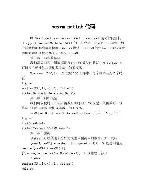
ocsvm matlab代码OC-SVM(One-Class Support Vector Machine)是支持向量机(Support Vector Machine, SVM)的一种变体,它只有一个类别,用于异常检测和离群点检测。
Matlab提供了OC-SVM的代码,下面将分步骤地介绍如何使用Matlab实现OC-SVM。
第一步:准备数据集我们需要准备一组数据进行OC-SVM算法的测试。
在Matlab中,可以很方便地创建随机数据集。
如下代码:X = randn(100,2); % 生成100个样本,每个样本具有2个特征figurescatter(X(:,1),X(:,2),'filled')title('Randomly Generated Data')第二步:训练模型我们可以使用fitcsvm函数来训练OC-SVM模型,此函数可在训练集上训练支持向量机分类器。
如下代码:svmModel = fitcsvm(X,'KernelFunction','rbf','Nu',0.05); figureplot(svmModel)title('Trained OC-SVM Model')第三步:预测现在我们可以使用训练好的模型来预测未知数据。
如下代码:[newX1,newX2] = meshgrid(linspace(-4,4)); % 创建网格点newX = [newX1(:) newX2(:)];[~,score] = predict(svmModel,newX); % 预测输出得分figurescatter(X(:,1),X(:,2),'filled')hold oncontour(newX1,newX2,reshape(score,size(newX1)),[00],'linewidth',2)title('Predicted Anomalies with the Trained OC-SVM Model') xlabel('Feature 1')ylabel('Feature 2')legend({'Normal Data','OC-SVM Predicted Anomalies'}) 第四步:结果分析在以上代码中,我们可以看到Matlab输出了预测结果,结果分为两部分,分别是好的结果和坏的结果。
支持向量机的smo算法(MATLABcode)

⽀持向量机的smo算法(MATLABcode)建⽴smo.m% function [alpha,bias] = smo(X, y, C, tol)function model = smo(X, y, C, tol)% SMO: SMO algorithm for SVM%%Implementation of the Sequential Minimal Optimization (SMO)%training algorithm for Vapnik's Support Vector Machine (SVM)%% This is a modified code from Gavin Cawley's MATLAB Support% Vector Machine Toolbox% (c) September 2000.%% Diego Andres Alvarez.%% USAGE: [alpha,bias] = smo(K, y, C, tol)%% INPUT:%% K: n x n kernel matrix% y: 1 x n vector of labels, -1 or 1% C: a regularization parameter such that 0 <= alpha_i <= C/n% tol: tolerance for terminating criterion%% OUTPUT:%% alpha: 1 x n lagrange multiplier coefficient% bias: scalar bias (offset) term% Input/output arguments modified by JooSeuk Kim and Clayton Scott, 2007global SMO;y = y';ntp = size(X,1);%recompute C% C = C/ntp;%initializeii0 = find(y == -1);ii1 = find(y == 1);i0 = ii0(1);i1 = ii1(1);alpha_init = zeros(ntp, 1);alpha_init(i0) = C;alpha_init(i1) = C;bias_init = C*(X(i0,:)*X(i1,:)' -X(i0,:)*X(i1,:)') + 1;%Inicializando las variablesSMO.epsilon = 10^(-6); SMO.tolerance = tol;SMO.y = y'; SMO.C = C;SMO.alpha = alpha_init; SMO.bias = bias_init;SMO.ntp = ntp; %number of training points%CACHES:SMO.Kcache = X*X'; %kernel evaluationsSMO.error = zeros(SMO.ntp,1); %errornumChanged = 0; examineAll = 1;%When all data were examined and no changes done the loop reachs its%end. Otherwise, loops with all data and likely support vector are%alternated until all support vector be found.while ((numChanged > 0) || examineAll)numChanged = 0;if examineAll%Loop sobre todos los puntosfor i = 1:ntpnumChanged = numChanged + examineExample(i);end;else%Loop sobre KKT pointsfor i = 1:ntp%Solo los puntos que violan las condiciones KKTnumChanged = numChanged + examineExample(i);end;end;end;if (examineAll == 1)examineAll = 0;elseif (numChanged == 0)examineAll = 1;end;end;alpha = SMO.alpha';alpha(alpha < SMO.epsilon) = 0;alpha(alpha > C-SMO.epsilon) = C;bias = -SMO.bias;model.w = (y.*alpha)* X; %%%%%%%%%%%%%%%%%%%%%%model.b = bias;return;function RESULT = fwd(n)global SMO;LN = length(n);RESULT = -SMO.bias + sum(repmat(SMO.y,1,LN) .* repmat(SMO.alpha,1,LN) .* SMO.Kcache(:,n))'; return;function RESULT = examineExample(i2)%First heuristic selects i2 and asks to examineExample to find a%second point (i1) in order to do an optimization step with two%Lagrange multipliersglobal SMO;alpha2 = SMO.alpha(i2); y2 = SMO.y(i2);if ((alpha2 > SMO.epsilon) && (alpha2 < (SMO.C-SMO.epsilon)))e2 = SMO.error(i2);elsee2 = fwd(i2) - y2;end;% r2 < 0 if point i2 is placed between margin (-1)-(+1)% Otherwise r2 is > 0. r2 = f2*y2-1r2 = e2*y2;%KKT conditions:% r2>0 and alpha2==0 (well classified)% r2==0 and 0% r2<0 and alpha2==C (support vectors between margins)%% Test the KKT conditions for the current i2 point.%% If a point is well classified its alpha must be 0 or if% it is out of its margin its alpha must be C. If it is at margin% its alpha must be between 0%take action only if i2 violates Karush-Kuhn-Tucker conditionsif ((r2 < -SMO.tolerance) && (alpha2 < (SMO.C-SMO.epsilon))) || ...((r2 > SMO.tolerance) && (alpha2 > SMO.epsilon))% If it doens't violate KKT conditions then exit, otherwise continue.%Try i2 by three ways; if successful, then immediately return 1;RESULT = 1;% First the routine tries to find an i1 lagrange multiplier that% maximizes the measure |E1-E2|. As large this value is as bigger% the dual objective function becames.% In this first test, only support vectors will be tested.POS = find((SMO.alpha > SMO.epsilon) & (SMO.alpha < (SMO.C-SMO.epsilon)));[MAX,i1] = max(abs(e2 - SMO.error(POS)));if ~isempty(i1)if takeStep(i1, i2, e2), return;end;end;%The second heuristic choose any Lagrange Multiplier that is a SV and tries to optimizefor i1 = randperm(SMO.ntp)if (SMO.alpha(i1) > SMO.epsilon) & (SMO.alpha(i1) < (SMO.C-SMO.epsilon))%if a good i1 is found, optimiseif takeStep(i1, i2, e2), return;end;endend%if both heuristc above fail, iterate over all data setfor i1 = randperm(SMO.ntp)if takeStep(i1, i2, e2), return;end;endend;end;%no progress possibleRESULT = 0;return;function RESULT = takeStep(i1, i2, e2)% for a pair of alpha indexes, verify if it is possible to execute% the optimisation described by Platt.global SMO;RESULT = 0;if (i1 == i2), return;end;% compute upper and lower constraints, L and H, on multiplier a2alpha1 = SMO.alpha(i1); alpha2 = SMO.alpha(i2);y1 = SMO.y(i1); y2 = SMO.y(i2);C = SMO.C; K = SMO.Kcache;s = y1*y2;if (y1 ~= y2)L = max(0, alpha2-alpha1); H = min(C, alpha2-alpha1+C);elseL = max(0, alpha1+alpha2-C); H = min(C, alpha1+alpha2);end;if (L == H), return;end;if (alpha1 > SMO.epsilon) & (alpha1 < (C-SMO.epsilon))e1 = SMO.error(i1);elsee1 = fwd(i1) - y1;end;%if (alpha2 > SMO.epsilon) & (alpha2 < (C-SMO.epsilon))% e2 = SMO.error(i2);%else% e2 = fwd(i2) - y2;%end;%compute etak11 = K(i1,i1); k12 = K(i1,i2); k22 = K(i2,i2);eta = 2.0*k12-k11-k22;%recompute Lagrange multiplier for pattern i2if (eta < 0.0)a2 = alpha2 - y2*(e1 - e2)/eta;%constrain a2 to lie between L and Hif (a2 < L)a2 = L;elseif (a2 > H)a2 = H;end;else%When eta is not negative, the objective function W should be%evaluated at each end of the line segment. Only those terms in the%objective function that depend on alpha2 need be evaluated...ind = find(SMO.alpha>0);aa2 = L; aa1 = alpha1 + s*(alpha2-aa2);Lobj = aa1 + aa2 + sum((-y1*aa1/2).*SMO.y(ind).*K(ind,i1) + (-y2*aa2/2).*SMO.y(ind).*K(ind,i2)); aa2 = H; aa1 = alpha1 + s*(alpha2-aa2);Hobj = aa1 + aa2 + sum((-y1*aa1/2).*SMO.y(ind).*K(ind,i1) + (-y2*aa2/2).*SMO.y(ind).*K(ind,i2)); if (Lobj>Hobj+SMO.epsilon)a2 = H;elseif (Lobj<Hobj-SMO.epsilon)a2 = L;elsea2 = alpha2;end;if (abs(a2-alpha2) < SMO.epsilon*(a2+alpha2+SMO.epsilon))return;end;% recompute Lagrange multiplier for pattern i1a1 = alpha1 + s*(alpha2-a2);w1 = y1*(a1 - alpha1); w2 = y2*(a2 - alpha2);%update threshold to reflect change in Lagrange multipliersb1 = SMO.bias + e1 + w1*k11 + w2*k12;bold = SMO.bias;if (a1>SMO.epsilon) & (a1<(C-SMO.epsilon))SMO.bias = b1;elseb2 = SMO.bias + e2 + w1*k12 + w2*k22;if (a2>SMO.epsilon) & (a2<(C-SMO.epsilon))SMO.bias = b2;elseSMO.bias = (b1 + b2)/2;end;end;% update error cache using new Lagrange multipliersSMO.error = SMO.error + w1*K(:,i1) + w2*K(:,i2) + bold - SMO.bias;SMO.error(i1) = 0.0; SMO.error(i2) = 0.0;% update vector of Lagrange multipliersSMO.alpha(i1) = a1; SMO.alpha(i2) = a2;%report progress madeRESULT = 1;return;画图⽂件:start_SMOforSVM.m(点击⾃动⽣成⼆维两类数据,画图,这⾥只是线性的,⾮线性的可以对应修改) clearX = []; Y=[];figure;% Initialize training data to empty; will get points from user% Obtain points froom the user:trainPoints=X;trainLabels=Y;clf;axis([-5 5 -5 5]);if isempty(trainPoints)% Define the symbols and colors we'll use in the plots latersymbols = {'o','x'};classvals = [-1 1];trainLabels=[];hold on; % Allow for overwriting existing plotsxlim([-5 5]); ylim([-5 5]);for c = 1:2title(sprintf('Click to create points from class %d. Press enter when finished.', c));[x, y] = getpts;plot(x,y,symbols{c},'LineWidth', 2, 'Color', 'black');% Grow the data and label matricestrainPoints = vertcat(trainPoints, [x y]);trainLabels = vertcat(trainLabels, repmat(classvals(c), numel(x), 1));endend% C = 10;tol = 0.001;% par = SMOforSVM(trainPoints, trainLabels , C, tol );% p=length(par.b); m=size(trainPoints,2);% if m==2% % for i=1:p% % plot(X(lc(i)-l(i)+1:lc(i),1),X(lc(i)-l(i)+1:lc(i),2),'bo')% % hold on% % end% k = -par.w(1)/par.w(2);% b0 = - par.b/par.w(2);% bdown=(-par.b-1)/par.w(2);% bup=(-par.b+1)/par.w(2);% for i=1:p% hold on% h = refline(k,b0(i));% set(hdown, 'Color', 'b')% hup=refline(k,bup(i));% set(hup, 'Color', 'b')% end% end% xlim([-5 5]); ylim([-5 5]);%% pauseC = 10;tol = 0.001;par = smo(trainPoints, trainLabels, C, tol);p=length(par.b); m=size(trainPoints,2);if m==2% for i=1:p% plot(X(lc(i)-l(i)+1:lc(i),1),X(lc(i)-l(i)+1:lc(i),2),'bo') % hold on% endk = -par.w(1)/par.w(2);b0 = - par.b/par.w(2);bdown=(-par.b-1)/par.w(2);bup=(-par.b+1)/par.w(2);for i=1:phold onh = refline(k,b0(i));set(h, 'Color', 'r')hdown=refline(k,bdown(i));set(hdown, 'Color', 'b')hup=refline(k,bup(i));set(hup, 'Color', 'b')endendxlim([-5 5]); ylim([-5 5]);。
matlab fitsvm参数
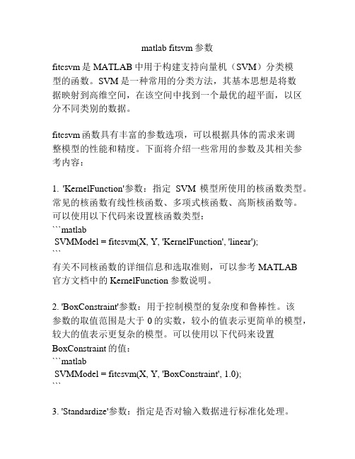
matlab fitsvm参数fitcsvm是MATLAB中用于构建支持向量机(SVM)分类模型的函数。
SVM是一种常用的分类方法,其基本思想是将数据映射到高维空间,在该空间中找到一个最优的超平面,以区分不同类别的数据。
fitcsvm函数具有丰富的参数选项,可以根据具体的需求来调整模型的性能和精度。
下面将介绍一些常用的参数及其相关参考内容:1. 'KernelFunction'参数:指定SVM模型所使用的核函数类型。
常见的核函数有线性核函数、多项式核函数、高斯核函数等。
可以使用以下代码来设置核函数类型:```matlabSVMModel = fitcsvm(X, Y, 'KernelFunction', 'linear');```有关不同核函数的详细信息和选取准则,可以参考MATLAB官方文档中的KernelFunction参数说明。
2. 'BoxConstraint'参数:用于控制模型的复杂度和鲁棒性。
该参数的取值范围是大于0的实数,较小的值表示更简单的模型,较大的值表示更复杂的模型。
可以使用以下代码来设置BoxConstraint的值:```matlabSVMModel = fitcsvm(X, Y, 'BoxConstraint', 1.0);```3. 'Standardize'参数:指定是否对输入数据进行标准化处理。
标准化是将输入数据减去其均值并除以标准差,以消除不同特征量级对模型的影响。
可以使用以下代码来设置是否进行标准化处理:```matlabSVMModel = fitcsvm(X, Y, 'Standardize', true);```更多关于数据标准化的信息可以参考MATLAB官方文档中的Standardize参数说明。
4. 'KernelScale'参数:用于指定核函数的缩放因子。
- 1、下载文档前请自行甄别文档内容的完整性,平台不提供额外的编辑、内容补充、找答案等附加服务。
- 2、"仅部分预览"的文档,不可在线预览部分如存在完整性等问题,可反馈申请退款(可完整预览的文档不适用该条件!)。
- 3、如文档侵犯您的权益,请联系客服反馈,我们会尽快为您处理(人工客服工作时间:9:00-18:30)。
支持向量机的matlab代码Matlab中关于evalin帮助:EVALIN(WS,'expression') evaluates 'expression' in the context of the workspace WS. WS can be 'caller' or 'base'. It is similar to EVAL except that you can control which workspace the expression is evaluated in.[X,Y,Z,...] = EVALIN(WS,'expression') returns output arguments from the expression.EVALIN(WS,'try','catch') tries to evaluate the 'try' expression and if that fails it evaluates the 'catch' expression (in the current workspace).可知evalin('base', 'algo')是对工作空间base中的algo求值(返回其值)。
如果是7.0以上版本>>edit svmtrain>>edit svmclassify>>edit svmpredictfunction [svm_struct, svIndex] = svmtrain(training, groupnames, varargin)%SVMTRAIN trains a support vector machine classifier%% SVMStruct = SVMTRAIN(TRAINING,GROUP) trains a support vector machine % classifier using data TRAINING taken from two groups given by GROUP.% SVMStruct contains information about the trained classifier that is% used by SVMCLASSIFY for classification. GROUP is a column vector of% values of the same length as TRAINING that defines two groups. Each% element of GROUP specifies the group the corresponding row of TRAINING % belongs to. GROUP can be a numeric vector, a string array, or a cell% array of strings. SVMTRAIN treats NaNs or empty strings in GROUP as% missing values and ignores the corresponding rows of TRAINING.%% SVMTRAIN(...,'KERNEL_FUNCTION',KFUN) allows you to specify the kernel % function KFUN used to map the training data into kernel space. The% default kernel function is the dot product. KFUN can be one of the% following strings or a function handle:%% 'linear' Linear kernel or dot product% 'quadratic' Quadratic kernel% 'polynomial' Polynomial kernel (default order 3)% 'rbf' Gaussian Radial Basis Function kernel% 'mlp' Multilayer Perceptron kernel (default scale 1)% function A kernel function specified using @,% for example @KFUN, or an anonymous function%% A kernel function must be of the form%% function K = KFUN(U, V)%% The returned value, K, is a matrix of size M-by-N, where U and V have M% and N rows respectively. If KFUN is parameterized, you can use% anonymous functions to capture the problem-dependent parameters. For % example, suppose that your kernel function is%% function k = kfun(u,v,p1,p2)% k = tanh(p1*(u*v')+p2);%% You can set values for p1 and p2 and then use an anonymous function:% @(u,v) kfun(u,v,p1,p2).%% SVMTRAIN(...,'POLYORDER',ORDER) allows you to specify the order of a% polynomial kernel. The default order is 3.%% SVMTRAIN(...,'MLP_PARAMS',[P1 P2]) allows you to specify the% parameters of the Multilayer Perceptron (mlp) kernel. The mlp kernel% requires two parameters, P1 and P2, where K = tanh(P1*U*V' + P2) and P1 % > 0 and P2 < 0. Default values are P1 = 1 and P2 = -1.%% SVMTRAIN(...,'METHOD',METHOD) allows you to specify the method used % to find the separating hyperplane. Options are%% 'QP' Use quadratic programming (requires the Optimization Toolbox)% 'LS' Use least-squares method%% If you have the Optimization Toolbox, then the QP method is the default% method. If not, the only available method is LS.%% SVMTRAIN(...,'QUADPROG_OPTS',OPTIONS) allows you to pass an OPTIONS % structure created using OPTIMSET to the QUADPROG function when using % the 'QP' method. See help optimset for more details.%% SVMTRAIN(...,'SHOWPLOT',true), when used with two-dimensional data,% creates a plot of the grouped data and plots the separating line for% the classifier.%% Example:% % Load the data and select features for classification% load fisheriris% data = [meas(:,1), meas(:,2)];% % Extract the Setosa class% groups = ismember(species,'setosa');% % Randomly select training and test sets% [train, test] = crossvalind('holdOut',groups);% cp = classperf(groups);% % Use a linear support vector machine classifier% svmStruct = svmtrain(data(train,:),groups(train),'showplot',true); % classes = svmclassify(svmStruct,data(test,:),'showplot',true);% % See how well the classifier performed% classperf(cp,classes,test);% cp.CorrectRate%% See also CLASSIFY, KNNCLASSIFY, QUADPROG, SVMCLASSIFY.% Copyright 2004 The MathWorks, Inc.% $Revision: 1.1.12.1 $ $Date: 2004/12/24 20:43:35 $% References:% [1] Kecman, V, Learning and Soft Computing,% MIT Press, Cambridge, MA. 2001.% [2] Suykens, J.A.K., Van Gestel, T., De Brabanter, J., De Moor, B., % Vandewalle, J., Least Squares Support Vector Machines,% World Scientific, Singapore, 2002.% [3] Scholkopf, B., Smola, A.J., Learning with Kernels,% MIT Press, Cambridge, MA. 2002.%% SVMTRAIN(...,'KFUNARGS',ARGS) allows you to pass additional% arguments to kernel functions.% set defaultsplotflag = false;qp_opts = [];kfunargs = {};setPoly = false; usePoly = false;setMLP = false; useMLP = false;if ~isempty(which('quadprog'))useQuadprog = true;elseuseQuadprog = false;end% set default kernel functionkfun = @linear_kernel;% check inputsif nargin < 2error(nargchk(2,Inf,nargin))endnumoptargs = nargin -2;optargs = varargin;% grp2idx sorts a numeric grouping var ascending, and a string grouping % var by order of first occurrence[g,groupString] = grp2idx(groupnames);% check group is a vector -- though char input is special...if ~isvector(groupnames) && ~ischar(groupnames)error('Bioinfo:svmtrain:GroupNotVector',...'Group must be a vector.');end% make sure that the data is correctly oriented.if size(groupnames,1) == 1groupnames = groupnames';end% make sure data is the right sizen = length(groupnames);if size(training,1) ~= nif size(training,2) == ntraining = training';elseerror('Bioinfo:svmtrain:DataGroupSizeMismatch',...'GROUP and TRAINING must have the same number of rows.')endend% NaNs are treated as unknown classes and are removed from the training % datanans = find(isnan(g));if length(nans) > 0training(nans,:) = [];g(nans) = [];。