CT图像三维重建(附源码)
医学CT三维重建
30
首都师范大学学报 (自然科学版)
2004 年
原始数据做“预处理”“, 图像重建”和“图像后续处 理”就可得到反映人体某断面几何结构的灰度图像. 例如 X 射线 CT ,此灰度图像反映了人体组织对 X 射 线的不同吸收系数 ,同一吸收系数具有相同的灰度 显示. 因为人体内不同组织的元素种类和密度不同 , 对 X 射线的吸收系数不同. 如果某一组织 (正常情 况下应具有相同的灰度) 的局部发生了病变 ,医生可 明显观察到此组织局部图像灰度的变化的直观显 示 ,从而帮助医生做出诊断.
下面分别对这几个过程中所涉及的关键技术进 行分析 :
1 获取断层图像信息
要进行三维重建 ,必须先得到清晰的二维断层 图像. 医学领域中 ,利用 X 射线 CT ,放射性核素 CT , 超声 CT 和核磁共振 CT 等技术获得人体断层图象. CT 图像向我们展示了人体内部有关病变的信息 ,把
© 1994-2010 China Academic Journal Electronic Publishing House. All rights reserved.
体素的获得有两种方法[4] : (1) 控制 CT 机使其 断层间隔减小 ,直至等于断层内的分辨率. 然而这将 增加检查成本 ,而且一般的 CT 机无法达到如此高 的分辨率. (2) 用计算机图像处理的方法 ,对现有的 断层图像进行插值运算 ,以获得立方体素表示的三 维物体. 插值后 ,断层图像数目增加 ,相当于层厚减 薄 ,这是国际上普遍采用的方法. 值得注意的是 ,插 值只是改变了断层间空间分辨率 ,使三维数据的处 理 、分析和显示更加方便 ,并没有产生新信息.
其次将医生感兴趣的组织从断层图像中分割开来再次在相邻两断层图像间进行内因为断层扫描间距一般比二维图像数据的象素尺寸要大以产生空间三个方向具有相同或相差不最后将重建后的三维图像数据在计算机屏幕上进行立体感显示要对它进行各种几何变换的运算实现多种投影显式方式及几何尺寸的测量等完成任意方位断层的重构任意方位立体视图手术摸拟和医学教学等
CT图像三维重建附源码
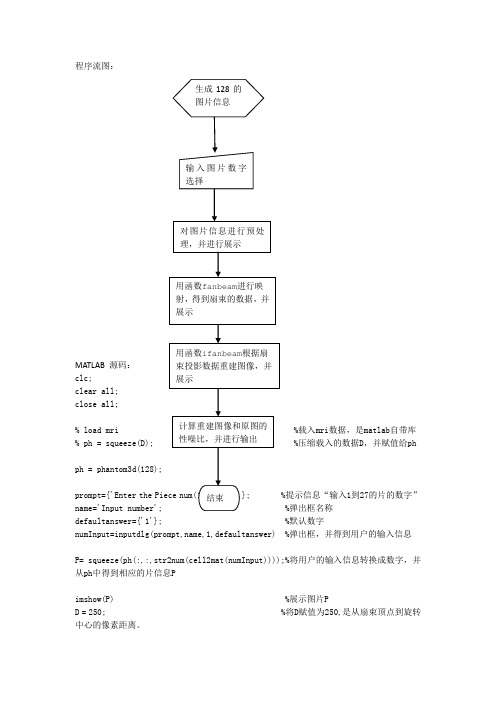
程序流图:MATLAB 源码: clc; clear all;close all;% load mri %载入mri 数据,是matlab 自带库 % ph = squeeze(D); %压缩载入的数据D ,并赋值给phph = phantom3d(128);prompt={'Enter the Piece num(1 to 128):'}; %提示信息“输入1到27的片的数字” name='Input number'; %弹出框名称defaultanswer={'1'}; %默认数字numInput=inputdlg(prompt,name,1,defaultanswer) %弹出框,并得到用户的输入信息P= squeeze(ph(:,:,str2num(cell2mat(numInput))));%将用户的输入信息转换成数字,并从ph 中得到相应的片信息Pimshow(P) %展示图片PD = 250; %将D 赋值为250,是从扇束顶点到旋转中心的像素距离。
生成128的图片信息 输入图片数字选择 对图片信息进行预处理,并进行展示 用函数fanbeam 进行映射,得到扇束的数据,并展示 用函数ifanbeam 根据扇束投影数据重建图像,并展示计算重建图像和原图的性噪比,并进行输出 结束dsensor1 = 2; %正实数指定扇束传感器的间距2F1 = fanbeam(P,D,'FanSensorSpacing',dsensor1); %通过P,D等计算扇束的数据值dsensor2 = 1; %正实数指定扇束传感器的间距1F2 = fanbeam(P,D,'FanSensorSpacing',dsensor2); %通过P,D等计算扇束的数据值dsensor3 = 0.25 %正实数指定扇束传感器的间距0.25 [F3, sensor_pos3, fan_rot_angles3] = fanbeam(P,D,...'FanSensorSpacing',dsensor3); %通过P,D等计算扇束的数据值,并得到扇束传感器的位置sensor_pos3和旋转角度fan_rot_angles3figure, %创建窗口imagesc(fan_rot_angles3, sensor_pos3, F3) %根据计算出的位置和角度展示F3的图片colormap(hot); %设置色图为hotcolorbar; %显示色栏xlabel('Fan Rotation Angle (degrees)') %定义x坐标轴ylabel('Fan Sensor Position (degrees)') %定义y坐标轴output_size = max(size(P)); %得到P维数的最大值,并赋值给output_sizeIfan1 = ifanbeam(F1,D, ...'FanSensorSpacing',dsensor1,'OutputSize',output_size);%根据扇束投影数据F1及D等数据重建图像figure, imshow(Ifan1) %创建窗口,并展示图片Ifan1title('图一');disp('图一和原图的性噪比为:');result=psnr1(Ifan1,P);Ifan2 = ifanbeam(F2,D, ...'FanSensorSpacing',dsensor2,'OutputSize',output_size);%根据扇束投影数据F2及D等数据重建图像figure, imshow(Ifan2) %创建窗口,并展示图片Ifan2disp('图二和原图的性噪比为:');result=psnr1(Ifan2,P);title('图二');Ifan3 = ifanbeam(F3,D, ...'FanSensorSpacing',dsensor3,'OutputSize',output_size);%根据扇束投影数据F3及D等数据重建图像figure, imshow(Ifan3) %创建窗口,并展示图片Ifan3title('图三');disp('图三和原图的性噪比为:');result=psnr1(Ifan3,P);function [p,ellipse]=phantom3d(varargin)%PHANTOM3D Three-dimensional analogue of MATLAB Shepp-Logan phantom% P = PHANTOM3D(DEF,N) generates a 3D head phantom that can% be used to test 3-D reconstruction algorithms.%% DEF is a string that specifies the type of head phantom to generate.% Valid values are:%% 'Shepp-Logan' A test image used widely by researchers in% tomography% 'Modified Shepp-Logan' (default) A variant of the Shepp-Logan phantom % in which the contrast is improved for better % visual perception.%% N is a scalar that specifies the grid size of P.% If you omit the argument, N defaults to 64.%% P = PHANTOM3D(E,N) generates a user-defined phantom, where each row% of the matrix E specifies an ellipsoid in the image. E has ten columns,% with each column containing a different parameter for the ellipsoids:%% Column 1: A the additive intensity value of the ellipsoid% Column 2: a the length of the x semi-axis of the ellipsoid% Column 3: b the length of the y semi-axis of the ellipsoid% Column 4: c the length of the z semi-axis of the ellipsoid% Column 5: x0 the x-coordinate of the center of the ellipsoid% Column 6: y0 the y-coordinate of the center of the ellipsoid% Column 7: z0 the z-coordinate of the center of the ellipsoid% Column 8: phi phi Euler angle (in degrees) (rotation about z-axis)% Column 9: theta theta Euler angle (in degrees) (rotation about x-axis)% Column 10: psi psi Euler angle (in degrees) (rotation about z-axis)%% For purposes of generating the phantom, the domains for the x-, y-, and% z-axes span [-1,1]. Columns 2 through 7 must be specified in terms% of this range.%% [P,E] = PHANTOM3D(...) returns the matrix E used to generate the phantom.%% Class Support% -------------% All inputs must be of class double. All outputs are of class double.%% Remarks% -------% For any given voxel in the output image, the voxel's value is equal to the% sum of the additive intensity values of all ellipsoids that the voxel is a% part of. If a voxel is not part of any ellipsoid, its value is 0.%% The additive intensity value A for an ellipsoid can be positive or negative;% if it is negative, the ellipsoid will be darker than the surrounding pixels.% Note that, depending on the values of A, some voxels may have values outside % the range [0,1].%% Example% -------% ph = phantom3d(128);% figure, imshow(squeeze(ph(64,:,:)))%% Copyright 2005 Matthias Christian Schabel (matthias @ stanfordalumni . org) % University of Utah Department of Radiology% Utah Center for Advanced Imaging Research% 729 Arapeen Drive% Salt Lake City, UT 84108-1218%% This code is released under the Gnu Public License (GPL). For more information, % see : /copyleft/gpl.html%% Portions of this code are based on phantom.m, copyrighted by the Mathworks %[ellipse,n] = parse_inputs(varargin{:});p = zeros([n n n]);rng = ( (0:n-1)-(n-1)/2 ) / ((n-1)/2);[x,y,z] = meshgrid(rng,rng,rng);coord = [flatten(x); flatten(y); flatten(z)];p = flatten(p);for k = 1:size(ellipse,1)A = ellipse(k,1); % Amplitude change for this ellipsoidasq = ellipse(k,2)^2; % a^2bsq = ellipse(k,3)^2; % b^2csq = ellipse(k,4)^2; % c^2x0 = ellipse(k,5); % x offsety0 = ellipse(k,6); % y offsetz0 = ellipse(k,7); % z offsetphi = ellipse(k,8)*pi/180; % first Euler angle in radianstheta = ellipse(k,9)*pi/180; % second Euler angle in radianspsi = ellipse(k,10)*pi/180; % third Euler angle in radianscphi = cos(phi);sphi = sin(phi);ctheta = cos(theta);stheta = sin(theta);cpsi = cos(psi);spsi = sin(psi);% Euler rotation matrixalpha = [cpsi*cphi-ctheta*sphi*spsi cpsi*sphi+ctheta*cphi*spsi spsi*stheta;-spsi*cphi-ctheta*sphi*cpsi -spsi*sphi+ctheta*cphi*cpsi cpsi*stheta;stheta*sphi -stheta*cphi ctheta];% rotated ellipsoid coordinatescoordp = alpha*coord;idx = find((coordp(1,:)-x0).^2./asq + (coordp(2,:)-y0).^2./bsq + (coordp(3,:)-z0).^2./csq <= 1);p(idx) = p(idx) + A;endp = reshape(p,[n n n]);return;function out = flatten(in)out = reshape(in,[1 prod(size(in))]);return;function [e,n] = parse_inputs(varargin)% e is the m-by-10 array which defines ellipsoids% n is the size of the phantom brain imagen = 128; % The default sizee = [];defaults = {'shepp-logan', 'modified shepp-logan', 'yu-ye-wang'};for i=1:narginif ischar(varargin{i}) % Look for a default phantom def = lower(varargin{i});idx = strmatch(def, defaults);if isempty(idx)eid = sprintf('Images:%s:unknownPhantom',mfilename);msg = 'Unknown default phantom selected.';error(eid,'%s',msg);endswitch defaults{idx}case 'shepp-logan'e = shepp_logan;case 'modified shepp-logan'e = modified_shepp_logan;case 'yu-ye-wang'e = yu_ye_wang;endelseif numel(varargin{i})==1n = varargin{i}; % a scalar is the image size elseif ndims(varargin{i})==2 && size(varargin{i},2)==10e = varargin{i}; % user specified phantomelseeid = sprintf('Images:%s:invalidInputArgs',mfilename);msg = 'Invalid input arguments.';error(eid,'%s',msg);endend% ellipse is not yet definedif isempty(e)e = modified_shepp_logan;endreturn;%%%%%%%%%%%%%%%%%%%%%%%%%%%%%% Default head phantoms: % %%%%%%%%%%%%%%%%%%%%%%%%%%%%%function e = shepp_logane = modified_shepp_logan;e(:,1) = [1 -.98 -.02 -.02 .01 .01 .01 .01 .01 .01];return;function e = modified_shepp_logan%% This head phantom is the same as the Shepp-Logan except% the intensities are changed to yield higher contrast in% the image. Taken from Toft, 199-200.%% A a b c x0 y0 z0 phi theta psi% -----------------------------------------------------------------e = [ 1 .6900 .920 .810 0 0 0 0 0 0-.8 .6624 .874 .780 0 -.0184 0 0 0 0-.2 .1100 .310 .220 .22 0 0 -18 0 10-.2 .1600 .410 .280 -.22 0 0 18 0 10.1 .2100 .250 .410 0 .35 -.15 0 0 0.1 .0460 .046 .050 0 .1 .25 0 0 0.1 .0460 .046 .050 0 -.1 .25 0 0 0.1 .0460 .023 .050 -.08 -.605 0 0 0 0.1 .0230 .023 .020 0 -.606 0 0 0 0.1 .0230 .046 .020 .06 -.605 0 0 0 0 ]; return;function e = yu_ye_wang%% Yu H, Ye Y, Wang G, Katsevich-Type Algorithms for Variable Radius Spiral Cone-Beam CT%% A a b c x0 y0 z0 phi theta psi% -----------------------------------------------------------------e = [ 1 .6900 .920 .900 0 0 0 0 0 0-.8 .6624 .874 .880 0 0 0 0 0 0-.2 .4100 .160 .210 -.22 0 -.25 108 0 0-.2 .3100 .110 .220 .22 0 -.25 72 0 0.2 .2100 .250 .500 0 .35 -.25 0 0 0.2 .0460 .046 .046 0 .1 -.25 0 0 0.1 .0460 .023 .020 -.08 -.65 -.25 0 0 0.1 .0460 .023 .020 .06 -.65 -.25 90 0 0.2 .0560 .040 .100 .06 -.105 .625 90 0 0-.2 .0560 .056 .100 0 .100 .625 0 0 0 ];return;% func——计算两幅图像的psnr值function result=psnr1(in1,in2)z=mse(in1,in2);result=10*log10(255.^2/z)% plot(result)function z=mse(x,y)if ndims(x)==3x=rgb2gray(x);endif ndims(y)==3y=rgb2gray(y);endx=double(x);y=double(y);[m1,n1]=size(x);[m2,n2]=size(y);m=min(m1,m2);n=min(n1,n2);z=0;for i=1:mfor j=1:nz=z+(x(i,j)-y(i,j)).^2;endendz=z/(m*n);。
CT三维重建指南.pdf
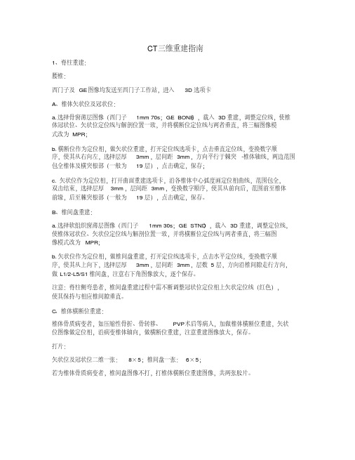
CT三维重建指南1、脊柱重建:腰椎:西门子及GE图像均发送至西门子工作站,进入3D选项卡A、椎体矢状位及冠状位:a. 选择骨窗薄层图像(西门子 1mm 70s;GE BONE),载入3D重建,调整定位线,使椎体冠状位、矢状位定位线与解剖位置一致,并将横断位定位线与两者垂直,将三幅图像模式改为MPR;b. 横断位作为定位相,做矢状位重建,打开定位线选项卡,点击垂直定位线,变换数字顺序,使其从右向左,选择层厚3mm,层间距3mm,方向平行于棘突-椎体轴线,两边范围包全椎体及横突根部(一般为19层),点击确定,保存;c. 矢状位作为定位相,打开曲面重建选项卡,沿各椎体中心弧度画定位相曲线,范围包全,双击结束,选择层厚3mm,层间距3mm,变换数字顺序,使其从前向后,范围前至椎体前缘,后至棘突根部(一般为19层),点击确定,保存。
B、椎间盘重建:a. 选择软组织窗薄层图像(西门子 1mm 30s;GE STND),载入3D重建,调整定位线,使椎体冠状位、矢状位定位线与解剖位置一致,并将横断位定位线与两者垂直,将三幅图像模式改为MPR;b. 矢状位作为定位相,做椎间盘重建,打开定位线选项卡,点击水平定位线,变换数字顺序,使其从上向下,选择层厚3mm,层间距3mm,层数5层,方向沿椎间隙走行方向,做L1/2-L5/S1椎间盘,注意右下角图像放大,逐个保存。
注意:脊柱侧弯患者,椎间盘重建过程中需不断调整冠状位定位相上矢状定位线(红色),使其保持与相应椎间隙垂直。
C、椎体横断位重建:椎体骨质病变者,如压缩性骨折、骨转移、PVP术后等病人,加做椎体横断位重建,矢状位图像做定位相,沿病变椎体轴向,做横断位重建,注意重建图像放大,保存。
打片:矢状位及冠状位二维一张:8×5;椎间盘一张:6×5;若为椎体骨质病变者,椎间盘图像不打,打椎体横断位重建图像,共两张胶片。
颈椎A、椎体矢状位及冠状位:a. 选择骨窗薄层图像(西门子 1mm 70s;GE BONE),载入3D重建,调整定位线,使椎体冠状位、矢状位定位线与解剖位置一致,并将横断位定位线与两者垂直,将三幅图像模式改为MPR;b. 横断位作为定位相,做矢状位重建,打开定位线选项卡,点击垂直定位线,变换数字顺序,使其从右向左,选择层厚3mm,层间距3mm,方向平行于棘突-椎体轴线,两边范围包全椎体及横突根部(一般为17-19层),点击确定,保存;c. 矢状位作为定位相,打开曲面重建选项卡,沿各椎体中心弧度画定位相曲线,范围包全,注意从斜坡开始,双击结束,选择层厚3mm,层间距3mm,变换数字顺序,使其从前向后,范围前至椎体前缘,后至棘突根部(一般为15-17层),点击确定,保存。
数学建模之CT的图像重建

Ax b min Axb xRn
2、无穷解的情形:
n
aij x j bi (i 1, 2, , n ) Ax b 无 穷 多 解
j 1
此时处理方式为: min xT x
Ax b s.t.Ax b
实践与思考题:P114,习题1
将待测物体的截面分成若干个体素每个体素为边长为的正方形设有一束射线的宽度为四模型的建立射线的强度以一定的速率被体素内的组织吸收而衰减衰减速率正比于该体素的衰减系个体素的射线密度为线性方程束射线我们就可以建如果有个体素记束射线穿过连续如果第射线的强度个体素的离开第射线的强度个体素的进入第射线密度为个体素的定义第99910将待检测的截面分成个体素并将它从束穿过个体素这些体素的编号为束穿过个体素这些体素的编号为其他所以式可写为若总共有束射线个体素这样ct图像重建的数学模型为
j1
ji1
(i1,2, ,n,k0,1,2, )
考 虑 方 程 组 : jn 1a aiijixja b iii (i1 ,2, ,n)
xik1xik
(bi
i1
aij
aii a j1 ii
xkj1jni1aaiiji
xkj)
(i1,2, ,n,k0,1,2, )
xk1 i
xik
( bi
某物 C质 值 T1的 00该 0物 水 质 水
CT值水1000水 水 水0
CT值 空 气10000 水 水1000
C T值 反 映 物 质 的 密 度 , 物 质 的 C T值 越 高 , 物 质 的 密 度 越 高
三、CT的结构与原理
平面CT的成像原理
体素、矩阵和象素
体 素:将选定层面分成若干个体积相同的立方体 数字矩阵:每个体素的X线衰减系数排列成矩阵 像 素:一幅CT的图象由许多按矩阵排列的小单元组 成,这些组成图象的基本单元称为像素
CT图像重建算法与三维可视化技术
CT图像重建算法与三维可视化技术医疗行业一直是科技创新的重点,特别是在影像学领域,病人的诊断和治疗都需要借助高科技的医疗设备和技术。
计算机断层扫描技术(CT)是一项主流技术,它可以非常精确地显示人体内部的结构和器官。
CT扫描产生的图像数据是由计算机三维图像重建算法进行处理,然后再通过三维可视化技术呈现出来。
一、CT扫描的原理和流程CT扫描使用的是一种非常特殊的X射线机器,它可以沿着不同的方向从多个角度对身体进行扫描,然后收集图像数据。
这些数据包含了身体内部所有的结构和器官信息,但是它们是以二维的方式呈现的,需要通过三维图像重建算法进行处理。
CT图像重建算法的基本原理是将二维扫描数据通过计算机进行处理,将它们转化为三维的模型图像,这些模型图像可以用来呈现人体结构和器官的实际情况。
CT图像重建算法的种类较多,常见的包括基于插值法的Feldkamp算法及其变种、基于迭代法的ART算法、基于傅里叶变换的FBP算法和统计学方法。
二、三维可视化技术三维可视化技术一直是科技发展的焦点,它是将虚拟的三维物体以真实的方式呈现在屏幕上。
医学界常用的三维可视化技术主要包括直接体绘制,光线追踪、容积渲染、表面重建等多种方式。
直接体绘制是指在三维模型中直接绘制三维物体的方法。
光线追踪可以在保持真实性的同时,采用光线追踪技术来求解物体的表现方式,这种方法可以表现阴影、反射和折射等效应。
容积渲染则是将数据集表示为一组体元素(voxel),并利用光线传播和有效的颜色映射技术来生成具有透明度和色彩信息的图像。
表面重建是将容积表面转换为三角形网格的过程,从而实现三维模型的表面可视化。
三、可视化技术在医学诊断中的应用三维可视化技术在医疗领域应用广泛,它可以以更加直观的方式呈现病人身体的结构和器官情况,帮助医生诊断和制定治疗方案。
比如,医生可以使用三维可视化技术对肿瘤、脊柱和骨骼等进行预览,预测手术效果,规划术前准备,进行手术操作。
同时,在教育领域,三维可视化技术还可以对疾病的发展变化进行演示,帮助学生更好地理解医学知识,提高教育效果和学术思考能力。
MATLAB编程实现连续断层工业CT图像的三维重建_张爱东
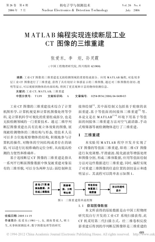
第26卷 第4期核电子学与探测技术V ol.26 N o.42006年 7月Nuclear Electr onics &Detection T echnolo gyJuly 2006M AT LA B 编程实现连续断层工业CT 图像的三维重建张爱东,李 炬,孙灵霞(中国工程物理研究院,四川绵阳621900)摘要:工业CT 图像的三维重建是无损检测领域的重要组成部分。
应用M A T L AB 编程,对连续多层工业CT 图像进行了三维重建,获得了具有较好立体感显示的三维图像,通过对三维图像的剖切、透明等显示,可以观察到物体的内部结构,得到了更直观和丰富的物体检测信息。
关键词:工业CT ;M A T L A B;三维重建中图分类号: T L99 文献标识码: A 文章编号: 0258-0934(2006)04-0489-03收稿日期:2005-11-19作者简介:张爱东(1981)),女,湖南娄底人,硕士生,从事核探测技术、数字图像处理等的研究工业CT 图像的三维重建技术综合了计算机图形学、计算机视觉和计算机图像处理等学科,是计算机科学可视化的重要组成部分,也是无损检测领域的一门重要技术。
通过二维序列断层图像重建出具有直观立体效果的图像,展现被检测物体的三维结构与形态,使技术人员可以多方位地观察物体的结构,积极地参与计算机的操作,对物体的空间结构或者存在的缺陷,可以进行比较准确的定位分析,从而提高检测的方便性和准确率。
基于连续断层CT 图像的三维重建是指从一系列平行断面图像数据中恢复被重建对象原有的三维形貌,可以分为两种方法:面绘制和直接体绘制[1],其中面绘制又包括基于轮廓的表面重建、基于等值面的间接体三维重建[2]等。
本论文是在M AT LAB [3,4]环境下用基于等值面的间接体三维重建方法对空气滤清器、手动式吸锡器等被检测物体进行了三维重建。
1 三维重建本实验用M ATLAB 程序开发并实现了CT 图像的等值面三维重建,即将二维CT 图像进行灰度调整、平滑滤波、锐化滤波等增强处理和图像分割,形成三维体数据,应用等值面绘制方法对这些数据进行三维重建;同时,编程实现了对重建三维图像的任意位置的剖切显示和透明显示。
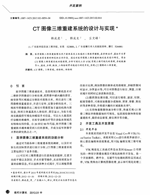
CT图像三维重建系统的设计与实现
2 开 发 工具 及 开发 原 理
2 . 1 开发平 台
本 系 统 采 用 的开 发 平 台 是 V i s u a l C + + 和V T K ( V i — s u a i z a t i 0 n T o o l k i t ) .系 统 采用 C + + 进行系统界面设计 、 核 心 算 法 编程 和 系 统 集 成 . 用 V T K编 程 实 现 三 维 可 视
床 实 践 提 供 可 视化 和 模 拟 手 术 信 息 ,可 以大 大 提 高 医
配准 等操作 , 可将 原始数据分成物体 、 背景 、 骨骼 、 软组 织等 多种类 型 . 并将感兴趣的区域提取 出来圆 。
( 3 ) 支持海量 数据快速 分析计算 . 快速 实现 C T图
像三维医学体数据场 的可视化 .包括面绘制 和体绘制
效地去除随机噪声 . 而 且 对 边 缘 的模 糊 程 度较 小 。
测 量 等 功 能
3 . 3 三 维 绘 制技 术
经过图像分割等二维处理 .把 图像 中感兴 趣的 区
域 提 取 出来 后 , 需 要 对 这 些 数 据 进行 三 维 绘 制 . 本 系统
三维绘制模块中使用 面绘制和体绘制技术进行重建 面绘 制处理 的是整个体 数据 场 中的小部分 数据 . 速度较快 .可 以快速灵活地对 图像进行 变换和旋转等 操作 面绘制重建 的只是物体表面 . 内部丰富信息无法
关 键 词 :CT 图像 ;三 维重 建 ;面绘 制 ;体 绘 制
0 引
言
的显示 比例 . 例如 图像 的整体 或局 部缩放 、 多幅 图像 同
时显 示 、 分屏显示等 ; 可 以 对 图像 进 行 标 注 、 测量 , 以便 在 阅 片 的 同时 记 录 获 取 的 信 息 。 ( 2 ) 提供 预处理 功能 , 可以进行 增强 、 滤波 、 切割 、
CT图像重建技术
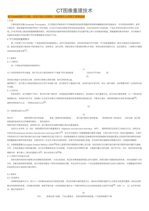
CT图像重建技术由于csdn贴图不⽅便,并且不能上传附件,我把原⽂上传到了资源空间1.引⾔计算机层析成像(Computed Tomography,CT)是通过对物体进⾏不同⾓度的射线投影测量⽽获取物体横截⾯信息的成像技术,涉及到放射物理学、数学、计算机学、图形图像学和机械学等多个学科领域。
CT技术不但给诊断医学带来⾰命性的影响.还成功地应⽤于⽆损检测、产品反求和材料组织分析等⼯业领域。
CT技术的核⼼是由投影重建图像的理论,其实质是由扫描所得到的投影数据反求出成像平⾯上每个点的衰减系数值。
图像重建的算法有很多,本⽂根据CT扫描机的发展对不同时期CT所采⽤重建算法分别进⾏介绍。
2. 平⾏束投影重建算法第⼀代和第⼆代CT机获取⼀个单独投影的采样数据是从⼀组平⾏射线获取的,这种采样类型叫平⾏投影。
平⾏投影重建算法⼀般分为直接法与间接法两⼤类。
直接法是直接计算线性⽅程系数的⽅法,如矩阵法、迭代法等。
间接法是先计算投影的傅⽴叶变换,再导出吸收系数的⽅法,如反投影法、⼆维傅⽴叶重建[1]。
法和滤波反投影法等2.1 直接法2.1.1 矩阵法设⼀个物体的内部吸收系数矩阵为:(1)为了求得该矩阵中的元素值,我们可以先计算该矩阵在T个⾓度下的T组投影值,如设⽔平⽅向时,则:(2)同样其它⾓度下也有类似⽅程,把所有⽅程联⽴得到求解,即可求得所有u值。
通常情况下,由于联⽴⽅程组的数⽬往往不同于未知数个数,且可能有不少重复的⽅程,这样形成的不是⽅阵,所以⼀般不满秩,此时需要利⽤⼴义逆矩阵法进⾏求解。
2.1.2 迭代法实际应⽤中,由于图像尺⼨较⼤,联⽴的⽅程个数较多,采⽤直接采⽤解析法难度较⼤,因此提出了迭代重建⽅法。
迭代法的主要思想是:从⼀个假设的初[2]。
始图像出发,采⽤迭代的⽅法,将根据⼈为设定并经理论计算得到的投影值同实验测得的投影值⽐较,不断进⾏逼近,按照某种最优化准则寻找最优解[2]:通常有两种迭代公式,⼀种是加法迭代公式(3)[2]:另⼀种是乘法迭代公式(4)两式中是相邻两次迭代的结果;是某⼀⾓度的实测投影值,是计算过程的计算投影值,是投影的某⼀射线穿过点的点数,即计算投影值的射线所经过的像素的数⽬,是松弛因⼦。
- 1、下载文档前请自行甄别文档内容的完整性,平台不提供额外的编辑、内容补充、找答案等附加服务。
- 2、"仅部分预览"的文档,不可在线预览部分如存在完整性等问题,可反馈申请退款(可完整预览的文档不适用该条件!)。
- 3、如文档侵犯您的权益,请联系客服反馈,我们会尽快为您处理(人工客服工作时间:9:00-18:30)。
程序流图:MATLAB 源码: clc;clear all;close all;% load mri %载入mri 数据,是matlab 自带库% ph = squeeze(D); %压缩载入的数据D ,并赋值给ph ph = phantom3d(128);prompt={'Enter the Piece num(1 to 128):'}; %提示信息“输入1到27的片的数字”name='Input number'; %弹出框名称defaultanswer={'1'}; %默认数字numInput=inputdlg(prompt,name,1,defaultanswer) %弹出框,并得到用户的输入信息 P= squeeze(ph(:,:,str2num(cell2mat(numInput))));%将用户的输入信息转换成数字,并从ph 中得到相应的片信息Pimshow(P) %展示图片PD = 250; %将D 赋值为250,是从扇束顶点到旋转中心的像素距离。
dsensor1 = 2; %正实数指定扇束传感器的间距2F1 = fanbeam(P,D,'FanSensorSpacing',dsensor1); %通过P ,D 等计算扇束的数据值 dsensor2 = 1; %正实数指定扇束传感器的间距1F2 = fanbeam(P,D,'FanSensorSpacing',dsensor2); %通过P ,D 等计算扇束的数据值dsensor3 = 0.25 %正实数指定扇束传感器的间距0.25 [F3, sensor_pos3, fan_rot_angles3] = fanbeam(P,D,...'FanSensorSpacing',dsensor3); %通过P ,D 等计算扇束的数据值,并得到扇束传感器的位置sensor_pos3和旋转角度fan_rot_angles3figure, %创建窗口imagesc(fan_rot_angles3, sensor_pos3, F3) %根据计算出的位置和角度展示F3的图片colormap(hot); %设置色图为hot colorbar; %显示色栏xlabel('Fan Rotation Angle (degrees)') %定义x 坐标轴ylabel('Fan Sensor Position (degrees)') %定义y 坐标轴output_size = max(size(P)); %得到P 维数的最大值,并赋值给output_size Ifan1 = ifanbeam(F1,D, ... 'FanSensorSpacing',dsensor1,'OutputSize',output_size);%根据扇束投影数据F1及D 等数据重建图像figure, imshow(Ifan1) %创建窗口,并展示图片Ifan1title('图一');disp('图一和原图的性噪比为:');result=psnr1(Ifan1,P);Ifan2 = ifanbeam(F2,D, ...'FanSensorSpacing',dsensor2,'OutputSize',output_size);%根据扇束投影数据F2及D 等数据重建图像figure, imshow(Ifan2) %创建窗口,并展示图片Ifan2disp('图二和原图的性噪比为:');result=psnr1(Ifan2,P);title('图二');Ifan3 = ifanbeam(F3,D, ...生成128的输入图片数字对图片信息进行预处用函数fanbeam 进行映射,得到扇束的数据,并用函数ifanbeam 根据扇束投影数据重建图像,并计算重建图像和原图的结束'FanSensorSpacing',dsensor3,'OutputSize',output_size);%根据扇束投影数据F3及D等数据重建图像figure, imshow(Ifan3) %创建窗口,并展示图片Ifan3title('图三');disp('图三和原图的性噪比为:');result=psnr1(Ifan3,P);function [p,ellipse]=phantom3d(varargin)%PHANTOM3D Three-dimensional analogue of MATLAB Shepp-Logan phantom% P = PHANTOM3D(DEF,N) generates a 3D head phantom that can% be used to test 3-D reconstruction algorithms.%% DEF is a string that specifies the type of head phantom to generate.% Valid values are:%% 'Shepp-Logan' A test image used widely by researchers in% tomography% 'Modified Shepp-Logan' (default) A variant of the Shepp-Logan phantom% in which the contrast is improved for better% visual perception.%% N is a scalar that specifies the grid size of P.% If you omit the argument, N defaults to 64.%% P = PHANTOM3D(E,N) generates a user-defined phantom, where each row% of the matrix E specifies an ellipsoid in the image. E has ten columns,% with each column containing a different parameter for the ellipsoids:%% Column 1: A the additive intensity value of the ellipsoid% Column 2: a the length of the x semi-axis of the ellipsoid% Column 3: b the length of the y semi-axis of the ellipsoid% Column 4: c the length of the z semi-axis of the ellipsoid% Column 5: x0 the x-coordinate of the center of the ellipsoid% Column 6: y0 the y-coordinate of the center of the ellipsoid% Column 7: z0 the z-coordinate of the center of the ellipsoid% Column 8: phi phi Euler angle (in degrees) (rotation about z-axis)% Column 9: theta theta Euler angle (in degrees) (rotation about x-axis) % Column 10: psi psi Euler angle (in degrees) (rotation about z-axis)%% For purposes of generating the phantom, the domains for the x-, y-, and % z-axes span [-1,1]. Columns 2 through 7 must be specified in terms% of this range.%% [P,E] = PHANTOM3D(...) returns the matrix E used to generate the phantom. %% Class Support% -------------% All inputs must be of class double. All outputs are of class double.%% Remarks% -------% For any given voxel in the output image, the voxel's value is equal to the% sum of the additive intensity values of all ellipsoids that the voxel is a% part of. If a voxel is not part of any ellipsoid, its value is 0.%% The additive intensity value A for an ellipsoid can be positive or negative;% if it is negative, the ellipsoid will be darker than the surrounding pixels.% Note that, depending on the values of A, some voxels may have values outside % the range [0,1].%% Example% -------% ph = phantom3d(128);% figure, imshow(squeeze(ph(64,:,:)))%% Copyright 2005 Matthias Christian Schabel (matthias @ stanfordalumni . org) % University of Utah Department of Radiology% Utah Center for Advanced Imaging Research% 729 Arapeen Drive% Salt Lake City, UT 84108-1218%% This code is released under the Gnu Public License (GPL). For more information, % see : /copyleft/gpl.html%% Portions of this code are based on phantom.m, copyrighted by the Mathworks %[ellipse,n] = parse_inputs(varargin{:});p = zeros([n n n]);rng = ( (0:n-1)-(n-1)/2 ) / ((n-1)/2);[x,y,z] = meshgrid(rng,rng,rng);coord = [flatten(x); flatten(y); flatten(z)];p = flatten(p);for k = 1:size(ellipse,1)A = ellipse(k,1); % Amplitude change for this ellipsoidasq = ellipse(k,2)^2; % a^2bsq = ellipse(k,3)^2; % b^2csq = ellipse(k,4)^2; % c^2x0 = ellipse(k,5); % x offsety0 = ellipse(k,6); % y offsetz0 = ellipse(k,7); % z offsetphi = ellipse(k,8)*pi/180; % first Euler angle in radianstheta = ellipse(k,9)*pi/180; % second Euler angle in radianspsi = ellipse(k,10)*pi/180; % third Euler angle in radianscphi = cos(phi);sphi = sin(phi);ctheta = cos(theta);stheta = sin(theta);cpsi = cos(psi);spsi = sin(psi);% Euler rotation matrixalpha = [cpsi*cphi-ctheta*sphi*spsi cpsi*sphi+ctheta*cphi*spsi spsi*stheta;-spsi*cphi-ctheta*sphi*cpsi -spsi*sphi+ctheta*cphi*cpsi cpsi*stheta;stheta*sphi -stheta*cphi ctheta];% rotated ellipsoid coordinatescoordp = alpha*coord;idx = find((coordp(1,:)-x0).^2./asq + (coordp(2,:)-y0).^2./bsq + (coordp(3,:)-z0).^2./csq <= 1);p(idx) = p(idx) + A;endp = reshape(p,[n n n]);return;function out = flatten(in)out = reshape(in,[1 prod(size(in))]);return;function [e,n] = parse_inputs(varargin)% e is the m-by-10 array which defines ellipsoids% n is the size of the phantom brain imagen = 128; % The default sizee = [];defaults = {'shepp-logan', 'modified shepp-logan', 'yu-ye-wang'};for i=1:narginif ischar(varargin{i}) % Look for a default phantomdef = lower(varargin{i});idx = strmatch(def, defaults);if isempty(idx)eid = sprintf('Images:%s:unknownPhantom',mfilename);msg = 'Unknown default phantom selected.';error(eid,'%s',msg);endswitch defaults{idx}case 'shepp-logan'e = shepp_logan;case 'modified shepp-logan'e = modified_shepp_logan;case 'yu-ye-wang'e = yu_ye_wang;endelseif numel(varargin{i})==1n = varargin{i}; % a scalar is the image size elseif ndims(varargin{i})==2 && size(varargin{i},2)==10e = varargin{i}; % user specified phantomelseeid = sprintf('Images:%s:invalidInputArgs',mfilename);msg = 'Invalid input arguments.';error(eid,'%s',msg);endend% ellipse is not yet definedif isempty(e)e = modified_shepp_logan;endreturn;%%%%%%%%%%%%%%%%%%%%%%%%%%%%%% Default head phantoms: % %%%%%%%%%%%%%%%%%%%%%%%%%%%%%function e = shepp_logane = modified_shepp_logan;e(:,1) = [1 -.98 -.02 -.02 .01 .01 .01 .01 .01 .01];return;function e = modified_shepp_logan%% This head phantom is the same as the Shepp-Logan except% the intensities are changed to yield higher contrast in% the image. Taken from Toft, 199-200.%% A a b c x0 y0 z0 phi theta psi% -----------------------------------------------------------------e = [ 1 .6900 .920 .810 0 0 0 0 0 0-.8 .6624 .874 .780 0 -.0184 0 0 0 0-.2 .1100 .310 .220 .22 0 0 -18 0 10-.2 .1600 .410 .280 -.22 0 0 18 0 10.1 .2100 .250 .410 0 .35 -.15 0 0 0.1 .0460 .046 .050 0 .1 .25 0 0 0.1 .0460 .046 .050 0 -.1 .25 0 0 0.1 .0460 .023 .050 -.08 -.605 0 0 0 0.1 .0230 .023 .020 0 -.606 0 0 0 0.1 .0230 .046 .020 .06 -.605 0 0 0 0 ];return;function e = yu_ye_wang%% Yu H, Ye Y, Wang G, Katsevich-Type Algorithms for Variable Radius Spiral Cone-Beam CT %% A a b c x0 y0 z0 phi theta psi% -----------------------------------------------------------------e = [ 1 .6900 .920 .900 0 0 0 0 0 0-.8 .6624 .874 .880 0 0 0 0 0 0-.2 .4100 .160 .210 -.22 0 -.25 108 0 0-.2 .3100 .110 .220 .22 0 -.25 72 0 0.2 .2100 .250 .500 0 .35 -.25 0 0 0.2 .0460 .046 .046 0 .1 -.25 0 0 0.1 .0460 .023 .020 -.08 -.65 -.25 0 0 0.1 .0460 .023 .020 .06 -.65 -.25 90 0 0.2 .0560 .040 .100 .06 -.105 .625 90 0 0-.2 .0560 .056 .100 0 .100 .625 0 0 0 ]; return;% func——计算两幅图像的psnr值function result=psnr1(in1,in2)z=mse(in1,in2);result=10*log10(255.^2/z)% plot(result)function z=mse(x,y)if ndims(x)==3x=rgb2gray(x);endif ndims(y)==3y=rgb2gray(y);endx=double(x);y=double(y);[m1,n1]=size(x);[m2,n2]=size(y);m=min(m1,m2);n=min(n1,n2);z=0;for i=1:mfor j=1:nz=z+(x(i,j)-y(i,j)).^2;endendz=z/(m*n);。