Violin plot
plot用法

plot用法Plot是一种在数据可视化和数据分析中广泛使用的工具。
它可以将数据以图形的形式呈现出来,帮助我们更好地理解和分析数据。
在本文中,我们将深入探讨plot的用法。
1. Plot的安装首先,我们需要安装plot。
在Python中,有很多库可以用于绘图,如matplotlib、seaborn等。
这些库都可以通过pip命令进行安装。
例如,要安装matplotlib库,可以在命令行中输入以下命令:```pip install matplotlib```2. Plot基础知识在使用plot之前,需要了解一些基础知识。
(1)图形类型plot支持各种类型的图形,包括线图、散点图、柱状图等。
(2)坐标系plot使用二维坐标系来绘制图形。
其中x轴表示一个变量,y轴表示另一个变量。
(3)数据格式plot需要输入一组或多组数据来绘制图形。
通常情况下,每组数据都是一个列表或数组。
3. Plot常见用法(1)线图线图是最常见的一种图形类型。
它通常用于显示连续变量之间的关系。
以下是一个简单的例子:```pythonimport matplotlib.pyplot as pltimport numpy as npx = np.arange(0, 10, 0.1)y = np.sin(x)plt.plot(x, y)plt.show()```这段代码将生成一个sin函数的图形。
(2)散点图散点图通常用于显示两个变量之间的关系。
以下是一个简单的例子:```pythonimport matplotlib.pyplot as pltimport numpy as npx = np.random.randn(100)y = np.random.randn(100)plt.scatter(x, y)plt.show()```这段代码将生成一个随机散点图。
(3)柱状图柱状图通常用于显示不同类别之间的比较。
以下是一个简单的例子:```pythonimport matplotlib.pyplot as pltx = ['A', 'B', 'C', 'D']y = [10, 20, 30, 40]plt.bar(x, y)plt.show()```这段代码将生成一个简单的柱状图。
seaborn 参数

seaborn 参数(原创实用版)目录1.Seaborn 简介2.Seaborn 参数的分类3.Seaborn 参数的具体使用方法4.Seaborn 参数的示例5.总结正文1.Seaborn 简介Seaborn 是一个 Python 库,用于创建美观的统计数据可视化。
Seaborn 的设计目标是方便用户快速制作出专业水平的统计图表,并且能够方便地集成到其他数据分析流程中。
Seaborn 基于 Matplotlib 库,因此可以使用 Matplotlib 的所有功能。
2.Seaborn 参数的分类Seaborn 参数主要分为以下几类:- 图形参数:用于控制图形的样式、颜色、线型等。
- 统计参数:用于控制统计数据的显示方式,例如均值、标准差等。
- 标签参数:用于控制图表的标签、标题等。
- 分格参数:用于控制图表的分格方式,例如行列分格、网格线等。
- 其他参数:包括一些其他控制图表显示的参数,例如图例、颜色映射等。
3.Seaborn 参数的具体使用方法Seaborn 参数的具体使用方法如下:- 使用 seaborn.plot() 函数创建图形,并传递所需的参数。
- 使用 seaborn.lineplot() 函数创建线图,并传递所需的参数。
- 使用 seaborn.barplot() 函数创建柱状图,并传递所需的参数。
- 使用 seaborn.scatterplot() 函数创建散点图,并传递所需的参数。
- 使用 seaborn.boxplot() 函数创建箱线图,并传递所需的参数。
- 使用 seaborn.violinplot() 函数创建小提琴图,并传递所需的参数。
4.Seaborn 参数的示例以下是一个 Seaborn 参数的示例:```pythonimport seaborn as snsimport matplotlib.pyplot as pltimport numpy as np# 创建数据x = np.linspace(0, 10, 100)y = np.sin(x)# 使用 seaborn.plot() 函数创建图形sns.plot(x, y, color="blue", linewidth=2, label="Sine Wave") # 使用 seaborn.lineplot() 函数创建线图sns.lineplot(x, y, color="red", linewidth=2, label="Sine Wave")# 使用 seaborn.barplot() 函数创建柱状图sns.barplot(x, y, color="green", linewidth=2, label="Sine Wave")# 使用 seaborn.scatterplot() 函数创建散点图sns.scatterplot(x, y, color="yellow", linewidth=2,label="Sine Wave")# 使用 seaborn.boxplot() 函数创建箱线图sns.boxplot(x, y, color="orange", linewidth=2, label="Sine Wave")# 使用 seaborn.violinplot() 函数创建小提琴图sns.violinplot(x, y, color="purple", linewidth=2, label="Sine Wave")# 显示图形plt.show()```5.总结Seaborn 参数是 Seaborn 库中用于控制图形样式、颜色、线型等的关键部分。
R语言绘图技巧导出高清图方法

R语⾔绘图技巧导出⾼清图⽅法
上⼀次⼩仙同学分享了 facet violin plot的画法,最后还卖了个关⼦,给⼤家留了个悬念。
科研⽂章的插图通常要求⽐较⾼,不仅要精准地展⽰出数据,选对图表类型,还需要简洁优美(?翻译成⼈话就是,同样的数据能不能多“卖”⼏分,就看图够不够⾼⼤上啦)。
⼩仙同学在画图的时候遇到的⼀个问题就是,RStudio直接导出的图,怎么这么不清晰?为什么教程⾥别⼈的图都那么清晰呢?这时候可能就有同学就会说,这还不简单,直接导出⽮量图不就可以了吗?
我们来看下,RStudio可以导出的图⽚格式有这么⼏种,⼩仙同学已经做过⼩⽩⿏替⼤家试了⼀遍,最合适的格式是EPS(其中⼩仙同学踩过好多坑,emf、svg、tiff、pdf都试过了,这⼏种格式的缺点各不同,总的来说,EPS最能满⾜我的需求,⾼清且易调整)。
我们先来看下导出的png图
对哦,⼩仙同学忘记告诉⼤家了,EPS格式的图可以⽤Adobe illustrator打开、编辑。
打开之后⿏标点⼀下就是下图这个样⼦,点击⿏标右键,选择取消编组
取消编组之后,这张图表⾥的元素就可以任意移动啦(这⾥请注意,有⼀些元素还是会是以组合的⽅式出现的,这时点击⿏标右键,选择释放剪切蒙版就可以啦)。
⼩仙同学把不想要的元素移⾛以后,然后导出tiff或者png就可以啦,放⼤图形也不会出现上图那种锯齿状的曲线。
好啦,今天⼩仙同学的分享就到这⾥啦。
RStudio导出EPS并在AI⾥编辑,就可以得到⾼清的图⽚啦,⽽且还可以任意编辑哦!更新⼀下,导出的pdf⽂件,也可以⽤AI打开进⾏类似的编辑,⽀持带有透明度的图⽚。
更多关于R语⾔导出⾼清图的资料请关注其它相关⽂章!。
violinplot函数

violinplot函数一、介绍violinplot函数是Python中的一个数据可视化函数,用于绘制小提琴图。
小提琴图是一种基于箱形图和核密度估计的数据可视化方法,可以更全面地展示数据的分布情况。
二、函数原型seaborn.violinplot(x=None, y=None, hue=None, data=None, order=None, hue_order=None, bw='scott', cut=2, scale='area', scale_hue=True, gridsize=100, width=0.8, inner='box',split=False, dodge=True, orient=None, linewidth=None,color=None, palette=None, saturation=0.75)三、参数说明1. x:x轴变量,可以是数值或分类变量。
2. y:y轴变量,必须是数值变量。
3. hue:用于分类的变量,可以将不同类别的数据用不同颜色表示。
4. data:用于绘制小提琴图的数据集。
5. order:x轴变量的排序方式。
6. hue_order:hue变量的排序方式。
7. bw:核密度估计中使用的带宽大小,默认为'scott'方法。
8. cut:核密度估计时截断尾部区域,默认为2.9. scale:控制小提琴图宽度和面积比例,默认为'area',即面积相等。
10. scale_hue:是否对hue进行缩放,默认为True.11. gridsize:控制核密度估计的精度,默认为100.12. width:小提琴图的宽度。
13. inner:小提琴图内部显示的内容,可以为'box','quartile','point'等。
14. split:是否将hue变量分开绘制,默认为False.15. dodge:是否对hue变量进行分离,默认为True.16. orient:小提琴图方向,可以为'v'(默认)或'h'。
R语言的“beanplot”包说明书

Package‘beanplot’October12,2022Type PackageTitle Visualization via Beanplots(Like Boxplot/Stripchart/ViolinPlot)Version1.3.1Date2022-04-09Author Peter KampstraMaintainer Peter Kampstra<*********************>Description Plots univariate comparison graphs,an alternative toboxplot/stripchart/violin plot.Suggests vioplot,latticeLicense GPL-2NeedsCompilation noRepository CRANDate/Publication2022-04-0907:22:29UTCR topics documented:beanplot-package (1)beanplot (2)Index7 beanplot-package Visualization via Beanplots(like Boxplot/Stripchart/Violin PlotDescriptionPlots univariate comparison graphs,alternative to boxplot/stripchart/violin plotDetails1Package:beanplotType:PackageVersion: 1.3.1Date:2022-04-09License:GPL-2The function beanplot does all the work.Author(s)Peter Kampstra<*********************>ReferencesKampstra,P.(2008)Beanplot:A Boxplot Alternative for Visual Comparison of Distributions.Jour-nal of Statistical Software,Code Snippets,28(1),1-9.doi:10.18637/jss.v028.c01See Alsographics vioplotExamplesbeanplot(rnorm(100),runif(100))if(interactive())vignette("beanplot",package="beanplot")beanplot Beanplot:A Boxplot/Stripchart/Vioplot AlternativeDescriptionPlots beans to compare the distributions of different groups;it draws one bean per group of data.A bean consists of a one-dimensional scatter plot,its distribution as a density shape and an average line for the distribution.Next to that,an overall average for the whole plot is drawn per default.Usagebeanplot(...,bw="SJ-dpi",kernel="gaussian",cut=3,cutmin=-Inf, cutmax=Inf,grownage=10,what=c(TRUE,TRUE,TRUE,TRUE),add=FALSE,col,axes=TRUE,log="auto",handlelog=NA,ll=0.16,wd=NA,maxwidth=0.8,maxstripline=0.96,method="stack",names,overallline="mean",beanlines=overallline,horizontal=FALSE,side="no",jitter=NULL,beanlinewd=2,frame.plot=axes,border=NULL,innerborder=NA,at=NULL,boxwex=1,ylim=NULL,xlim=NULL,s=NA)Arguments...data which to perform the beanplot on.This data can consist of dataframes, vectors and/or formulas.For each formula,a dataset can be specified withdata=[dataset],and a subset can be specified with subset=[subset].If subset/dataarguments are passed,but there are not enough subset/data arguments,they arereused.Additionally,na.action,drop.unused.levels and xlev can be passed tomodel.frame in the same way.Also,parameters for axis and title can bepassed.bw the bandwidth(method)being used,used by density.In case of a method,the average computed bandwidth is used.kernel see density.cut the beans are cut beyond cut*bwcutmin the low-ends of the beans are cut below mincut*bw.Defaults to cut.cutmax the high-ends of the beans are cut beyond maxcut*bw.Defaults to cut.grownage the width of a bean grows linearly with the count of points,until grownage is reached.what a vector of four booleans describing what to plot.In the following order,these booleans stand for the total average line,the beans,the bean average,and thebeanlines.For example,what=c(0,0,0,1)produces a stripchart add if true,do not start a new plotcol the colors to be used.A vector of up to four colors can be used.In the following order,these colors stand for the area of the beans(without the border,use borderfor that color),the lines inside the bean,the lines outside the bean,and theaverage line per bean.Transparent colors are supported.col can be a list ofcolor vectors,the vectors are then used per bean,and reused if necessary.axes if false,no axes are drawn.log use log="y"or log=""to force a log-axis.In case of log="auto",a log-transformation is used if appropriatehandlelog if handlelog then all the calculations are done using a log-scale.By default this is determined using the log parameter.ll the length of the beanline per point found.wd the linear transformation that determines the width of the beans.By default determined using maxwidth,and returned.maxwidth the maximum width of a bean.maxstripline the maximum length of a beanline.method the method used when two points on a bean are the same."stack","overplot"and"jitter"are supported.names a vector of names for the groups.overallline the method used for determining the overall line.Defaults to"mean","median"is also supported.beanlines the method used for determining the average bean line(s).Defaults to"mean", "median"and"quantiles"are also supported.horizontal if true,the beanplot is horizontalside the side on which the beans are plot.Default is"no",for symmetric beans."first","second"and"both"are also supported.jitter passed to jitter as amount in case of method="jitter".beanlinewd the width used for the average bean lineframe.plot if true,plots a frame.border the color for the border around a bean.NULL for par("fg"),NA for no border.If border is a vector,it specifies the color per bean,and colors are reused ifnecessary.innerborder a color(vector)for the border inside the bean(s).Especially useful if side="both".Use NA for no inner border.Colors are reused if necessary.The inner border isdrawn as the last step in the drawing process.at the positions at which a bean should be drawn.boxwex a scale factor applied to all patible with boxplot.ylim the range to plot.xlim the range to plot the beans at.s if true,plots the names as axis labelsDetailsUse the"what"parameter to omit certain parts from drawing.Most parameters are compatible with boxplot and stripchart.For compatibility,arguments with the name"formula"or"x"are used as data.However,data or formulas do not need to be named"x"or"formula".The function handles (combinations of)dataframes,vectors and/or formulas.Valuebw the bandwidth(bw)used.wd the bean width(wd)used.names a vector of names for the groups.stats a vector of statistics calculated for the beanlines.overall statistic calculated for the overall line.log log axis that was selected.ylim ylim that was used.xlim xlim that was used.NoteIn case of more than5000values per bean,the autodetection of the log parameter is approximated.In such cases,use log=""or log="y".Also,the what parameter can help to omit parts that are not useful in certain plots,and take time to draw.Author(s)Peter Kampstra<*********************>ReferencesKampstra,P.(2008)Beanplot:A Boxplot Alternative for Visual Comparison of Distributions.Jour-nal of Statistical Software,Code Snippets,28(1),1-9.doi:10.18637/jss.v028.c01See Alsoboxplot,stripchart,density,rug,vioplot in package vioplotExamplesbeanplot(rnorm(22),rnorm(22),rnorm(22),main="Test!",rnorm(3))#mostly examples taken from boxplot:par(mfrow=c(1,2))boxplot(count~spray,data=InsectSprays,col="lightgray")beanplot(count~spray,data=InsectSprays,col="lightgray",border="grey",cutmin=0) boxplot(count~spray,data=InsectSprays,col="lightgray")beanplot(count~spray,data=InsectSprays,col="lightgray",border="grey", overallline="median")boxplot(decrease~treatment,data=OrchardSprays,log="y",col="bisque",ylim=c(1,200))beanplot(decrease~treatment,data=OrchardSprays,col="bisque",ylim=c(1,200))par(mfrow=c(2,1))mat<-cbind(Uni05=(1:100)/21,Norm=rnorm(100),T5=rt(100,df=5),Gam2=rgamma(100,shape=2))par(las=1)#all axis labels horizontalboxplot(data.frame(mat),main="boxplot(*,horizontal=TRUE)",horizontal=TRUE,ylim=c(-5,8))beanplot(data.frame(mat),main="beanplot(*,horizontal=TRUE)",horizontal=TRUE,ylim=c(-5,8))par(mfrow=c(1,2))boxplot(len~dose,data=ToothGrowth,boxwex=0.25,at=1:3-0.2,subset=supp=="VC",col="yellow",main="Guinea Pigs Tooth Growth",xlab="Vitamin C dose mg",ylab="tooth length",ylim=c(-1,40),yaxs="i")boxplot(len~dose,data=ToothGrowth,add=TRUE,boxwex=0.25,at=1:3+0.2,subset=supp=="OJ",col="orange")legend("bottomright",bty="n",c("Ascorbic acid","Orange juice"),fill=c("yellow","orange"))allplot<-beanplot(len~dose+supp,data=ToothGrowth,what=c(TRUE,FALSE,FALSE,FALSE),s=FALSE,ylim=c(-1,40),yaxs="i") beanplot(len~dose,data=ToothGrowth,add=TRUE,boxwex=0.6,at=1:3*2-0.9,subset=supp=="VC",col="yellow",border="yellow2",main="Guinea Pigs Tooth Growth",xlab="Vitamin C dose mg",ylab="tooth length",ylim=c(3,40),yaxs="i",bw=allplot$bw,wd=allplot$wd,what=c(FALSE,TRUE,TRUE,TRUE)) beanplot(len~dose,data=ToothGrowth,add=TRUE,boxwex=0.6,at=1:3*2-0.1,subset=supp=="OJ",col="orange",border="darkorange",bw=allplot$bw,wd=allplot$wd,what=c(FALSE,TRUE,TRUE,TRUE)) legend("bottomright",bty="n",c("Ascorbic acid","Orange juice"), fill=c("yellow","orange"))par(mfrow=c(1,2))boxplot(len~dose,data=ToothGrowth,boxwex=0.25,at=1:3-0.2,subset=supp=="VC",col="yellow",main="Guinea Pigs Tooth Growth",xlab="Vitamin C dose mg",ylab="tooth length",ylim=c(-1,40),yaxs="i")boxplot(len~dose,data=ToothGrowth,add=TRUE,boxwex=0.25,at=1:3+0.2,subset=supp=="OJ",col="orange")legend("bottomright",bty="n",c("Ascorbic acid","Orange juice"), fill=c("yellow","orange"))beanplot(len~reorder(supp,len,mean)*dose,ToothGrowth,side="b",col=list("yellow","orange"),border=c("yellow2", "darkorange"),main="Guinea Pigs Tooth Growth",xlab="Vitamin C dose mg",ylab="tooth length",ylim=c(-1,40),yaxs="i")legend("bottomright",bty="n",c("Ascorbic acid","Orange juice"), fill=c("yellow","orange"))#Example with multiple vectors and/or formulaspar(mfrow=c(2,1))beanplot(list(all=ToothGrowth$len),len~supp,ToothGrowth,len~dose) title("Tooth growth length(beanplot)")#Trick using internal functions to do this with other functions:mboxplot<-function(...){graphics::boxplot(beanplot:::getgroupsfromarguments(),...)}mstripchart<-function(...,method="overplot",jitter=0.1,offset=1/3, vertical=TRUE,s,add=FALSE,at=NULL,xlim=NULL,ylim=NULL,ylab=NULL,xlab=NULL,dlab="",glab="",log="",pch=0,col=par("fg"),cex=par("cex"),axes=TRUE,frame.plot=axes){graphics::stripchart(beanplot:::getgroupsfromarguments(),method,jitter,offset,vertical,s,add,at,xlim,ylim,ylab,xlab,dlab,glab,log,pch,col,cex,axes,frame.plot)}mstripchart(list(all=ToothGrowth$len),len~supp,ToothGrowth,len~dose, xlim=c(0.5,6.5))title("Tooth growth length(stripchart)")Index∗hplotbeanplot,2∗packagebeanplot-package,1axis,3beanplot,2,2beanplot-package,1boxplot,4,5density,3,5graphics,2jitter,4model.frame,3rug,5stripchart,3–5title,3vioplot,2,57。
箱线图和小提琴图合在一起更好

欢迎加入微生信生物 快来微生信生物
微生信生物
将箱子换成小提琴:geom_violin # Violin basic data %>% ggplot( aes(x=name, y=value, fill=name)) + geom_violin() + scale_fill_viridis(discrete = TRUE, alpha=0.6, option="A") + theme_ipsum() + theme( legend.position="none", plot.title = element_text(size=11) )+ ggtitle("Violin chart") + xlab("")
小提琴和箱线图还是放一起的好
# Libraries library(ggplot2) library(dplyr) library(hrbrthemes) library(viridis)
# create a dataset data <- data.frame( name=c( rep("A",500), rep("B",500), rep("B",500), rep("C",20), rep('D', 100) ), value=c( rnorm(500, 10, 5), rnorm(500, 13, 1), rnorm(500, 18, 1), rnorm(20, 25, 4), rnorm(100, 12, 1) ) )
# custom boxes color="blue", fill="blue", alpha=0.2,
matlab violinplot 参数
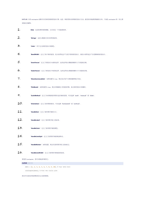
MATLAB 中的violinplot函数可以用来绘制核密度估计图,这是一种新型的非参数密度估计方法,能更真实地描绘数据的分布。
下面是violinplot的一些主要参数及其解释:1.Data: 这是您要绘制的数据。
它应该是一个向量或矩阵。
2.'Strings': 这是与数据点对应的类别标签。
3.'Color': 用于定义核密度估计的颜色。
4.'BandWidth': 定义了每个核的宽度。
较大的带宽会产生更平滑的密度估计,而较小的带宽会产生更精细的密度估计。
5.'InnerFences': 定义了密度估计内部的边界,这些边界表示数据的概率大于该值的区域。
6.'OuterFences': 定义了密度估计外部的边界,这些边界表示数据的概率小于该值的区域。
7.'ShowSummaryStats': 如果设置为true,则会显示每个分箱的摘要统计信息。
8.'PlotBands': 如果设置为true,则会在数据值上绘制条形图,表示核密度估计的概率。
9.'ScaleMethod': 定义了如何缩放条形图以适应轴的范围。
可以选择'auto'、'manual' 或'data'。
10.'Orientation': 定义了条形图的取向。
可以选择'horizontal' 或'vertical'。
11.'HandleSize': 定义了条形图手柄的大小。
12.'HandleLabel': 定义了条形图手柄上的标签。
13.'HandleColor': 定义了条形图手柄的颜色。
14.'HandleLineStyle': 定义了条形图手柄的线条样式。
violin小提琴的相关英文表达

The violin is a bowed string instrument with four strings usually tuned in perfect fifths. It is the smallest and highestpitched member of the violin family of string instruments, which also includes the viola and cello.
Chen Mei and electric violin
Musical styles
1 ,Classical music:Since the Baroque era, the violin has been one of the most important of all instruments.
An electric violin is a violin equipped with an electric signal output of its sound, and is generally considered to be a specially constructed instrument which can either be: 1,an electro-acoustic violin capable of producing both acoustic sound and electric signal 2,an electric violin capable of producing only electric siiccolò Paganini,1782-1840) 亨里克· 维尼亚夫斯基(Henryk Wieniawski 1835 – 1880) 莱奥波德· 奥尔(Leopold Auer 1845-1930) 弗里茨· 克莱斯勒(Fritz Kreisler,1875—1962) 乔治· 埃内斯库(Georges Enescu,1881—1955) 亚沙· 海菲兹(Jascha Heifetz,1901—1987) 大卫· 奥伊斯特拉赫(David Oistrach,1908—1974) 耶胡迪· 梅纽因(Yehudi Menuhin,1916—1999) 艾萨克· 斯特恩(Isaac Stern,1920—2001) 约舍夫‧哈西德 (Josef Hassid,1923-1950) 列奥尼德· 柯岗(Leonid Kogan,1924—1982) 米高· 拉宾 (Michael Rabin,1936—1972) 萨尔瓦托雷· 阿卡多(Salvatore Accardo,1941—) 伊扎克· 帕尔曼(Itzhak Perlman,1945—) 平夏斯· 祖克曼(Pinchas Zukerman,1948—) 安娜-苏菲· 穆特 (Anne Sophie Mutter, 1963—) 俞丽拿 盛中国 薛伟 马思聪 盛中国 西崎崇子 吕思清 陈美 林昭亮 蔡佳龙(Chia-Long Tsai,1978—) 黄蒙拉 (Mengla Huang, 1980—) 李传韵 (Chuanyun Li, 1980—) 吴迪 (Di Wu, 1987—)
- 1、下载文档前请自行甄别文档内容的完整性,平台不提供额外的编辑、内容补充、找答案等附加服务。
- 2、"仅部分预览"的文档,不可在线预览部分如存在完整性等问题,可反馈申请退款(可完整预览的文档不适用该条件!)。
- 3、如文档侵犯您的权益,请联系客服反馈,我们会尽快为您处理(人工客服工作时间:9:00-18:30)。
Violin plot
小提琴图绘制数字数据的方法。
小提琴是箱线图和密度分布的一个组合。
具体地说,它开始以一个盒形图。
然后,它增加了一个密度分布
用JMP作小提琴图
例:数据(两组变量:月份;登陆次数。
)
首先,以箱线图对数据做图表。
对登陆次数分布进行作图。
可以很直观的看到登陆次数的分散情况。
但是不能清楚的看到各个登陆次数区间段的分布情况,不知道登陆次数在5-10跟25-30哪个区间段的人比较多。
再来,作小提琴图
在JMP窗口中打开文件,选择“图形”-“图形生成器”
把“登陆次数”作为Y变量,选择“小提琴”图标
得到以下的小提琴图
可以看出小提琴图比箱线图更清楚的反映出分散密度情况,可以看出登陆次数各个区间段的登陆次数分布情况。
这幅图看以看出登陆次数在25,18,3附近的人最多。
按第一列月份作为X变量分组。