高斯光束瑞利长度
高斯光束的特性实验
实验二 高斯光束的测量一 实验目的1.熟悉基模光束特性。
2.掌握高斯光速强度分布的测量方法。
3.测量高斯光速的远场发散角。
二 实验原理众所周知,电磁场运动的普遍规律可用Maxwell 方程组来描述。
对于稳态传输光频电磁场可以归结为对光现象起主要作用的电矢量所满足的波动方程。
在标量场近似条件下,可以简化为赫姆霍兹方程,高斯光束是赫姆霍兹方程在缓变振幅近似下的一个特解,它可以足够好地描述激光光束的性质。
使用高斯光束的复参数表示和ABCD 定律能够统一而简洁的处理高斯光束在腔内、外的传输变换问题。
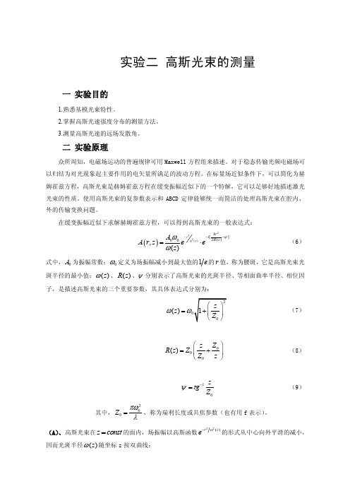
在缓变振幅近似下求解赫姆霍兹方程,可以得到高斯光束的一般表达式:()222()[]2()00,()r z kr i R z A A r z e e z ωψωω---=⋅ (6)式中,0A 为振幅常数;0ω定义为场振幅减小到最大值的1的r 值,称为腰斑,它是高斯光束光斑半径的最小值;()z ω、()R z 、ψ分别表示了高斯光束的光斑半径、等相面曲率半径、相位因子,是描述高斯光束的三个重要参数,其具体表达式分别为:()z ωω=(7) 000()Z z R z Z Z z ⎛⎫=+ ⎪⎝⎭(8)10z tg Z ψ-= (9) 其中,200Z πωλ=,称为瑞利长度或共焦参数(也有用f 表示)。
(A )、高斯光束在z const =的面内,场振幅以高斯函数22()r z eω-的形式从中心向外平滑的减小,因而光斑半径()z ω随坐标z 按双曲线:2200()1z z Z ωω-= (10)规律而向外扩展,如图四所示高斯光束以及相关参数的定义图四(B )、 在(10)式中令相位部分等于常数,并略去()z ψ项,可以得到高斯光束的等相面方程: 22()r z const R z += (11) 因而,可以认为高斯光束的等相面为球面。
(C )、瑞利长度的物理意义为:当0z Z =时,00()Z ω。
在实际应用中通常取0z Z =±范围为高斯光束的准直范围,即在这段长度范围内,高斯光束近似认为是平行的。
Zemax 2003 中高斯光束计算步骤
Zemax 2003 中步骤:Anaylsis-calculations-gaussian beam中计算高斯光束传输(快捷键 ctrl +B)Gaussian beam data-setting中初始高斯光束参数设置:M2:光束的模式,为大于1的整数,1为单基模,大于1为多模。
Surf 1 to Waist:1面距离束腰的距离,因此一般做法是在物面和光学组前插一个1面,将束腰“放在”1面上。
Divergence:远场发散角。
Radius:光波的半径,束腰处无穷大。
Rayleigh:瑞利长度,这三个随便一本激光原理的书里都有。
目前我的一个认识:高斯光束计算在zemax 2003中可以也只能计算束腰尺寸,位置,远场发散角等,欢迎大家相互交流。
Email: boooq@by hust—booq 2008-1-26PS:没有时间翻译,在这里把Zemax里所有有关资料汇总一下,给出一个简单案例。
-=-=-=-=-=--=-=-=-=-=--=-=-=-=-=--=-=-=-=-=--=-=-=-=-=--=-=-=-=-=-高斯光束Zemax介绍Computes Gaussian beam parameters.Wavelength: The wavelength number to use for the calculation.M2 Factor: The M2 quality factor used to simulate mixed mode beams. See the Discussion.Waist Size: The radial size of the embedded (perfect TEM00 mode) beam waist in object space in lens units.Surf 1 to Waist: The distance from surface 1 (NOT the object surface) to the beam waist location. This parameter will be negative if the waist lies to the left of surface 1.Update, Orient, Surface: See below.Discussion: This feature computes ideal and aberrated Gaussian beam data, such as beam size, beam divergence, and waist locations, as a given input beam propagates through the lens system. This discussion is not meant to be a complete tutorial on laser beam propagation theory. For more information on Gaussian beam propagation, see one of the following references: "Lasers", A. E. Siegman, University Science Books (1986), "Gaussian beam ray-equivalent modeling and optical design", R. Herloski, S. Marshall, and R. Antos, Applied Optics Vol. 22, No. 8 pp. 1168 (1983), "Beam characterization and measurement of propagation attributes", M. W. Sasnett and T. F. Johnson, Jr., Proc. SPIE Vol. 1414, pp 21 (1991), and "New developments in laser resonators", A. E. Siegman, Proc. SPIE Vol. 1224, pp 2 (1990).A Gaussian laser beam is described by a beam waist size, a wavelength, and a location in object space. The Gaussian beam is an idealization that can be approached but never attained in practice. However, real laser beams can be well described by an embedded Gaussian beam with ideal characteristics, and a quality factor, called M2, which defines the relative beam size and divergence with respect to theembedded Gaussian mode. The ideal M2 value is unity, but real lasers will always have an M2 value greater than unity.This feature requires the definition of the initial input embedded beam properties, and the M2 value. The input embedded beam is defined by the location of the input beam waist relative to surface 1 (note this is not the object surface, but the first surface after the object) and the waist radial size at this location. ZEMAX then propagates this embedded beam through the lens system, and at each surface the beam data is computed and displayed in the output window. ZEMAX computes the Gaussian beam parameters for both X and Y orientations.Default beam parameters:ZEMAX defaults to a waist size of 0.05 lens units (no matter what the lens units are) and a surface 1 to waist distance of zero; this of course means the waist is at surface 1. The default values may be reset by clicking on the "Reset" button. After the default values are computed and displayed, any alternate beam waist size and location may be entered and that Gaussian beam will be traced instead.Propagating the embedded beam:Once the initial beam waist and location parameters are established, ZEMAX traces the embedded beam through the system and computes the radial beam size, the narrowest radial waist, the surface coordinate relative to the beam waist, the phase radius of curvature of the beam, the semi-divergence angle, and the Rayleigh range for every surface in the system. ZEMAX calls these parameters the Size, Waist, Waist Z, Radius, Divergence, and Rayleigh, respectively, on the text listing that is generated.The quality factor:All of the preceding results are correct for the ideal embedded Gaussian beam. For aberrated,mixed-mode beams, a simple extension to the fundamental Gaussian beam model has been developed by Siegman. The method uses a term called the beam quality factor, usually denoted by M2. The factor M2 can be though of as "times diffraction limited" number, and is always greater than unity. The M2 factor determines the size of the real, aberrated Gaussian beam by scaling the size and divergence of the embedded Gaussian mode by M. It is common practice to specify M2 for a laser beam, rather than M, although the factor M is used to scale the beam size. The M2 factor must be measured to be determined correctly. If the M2 factor is set to unity, the default value, ZEMAX simply computes the TEM00 data described above. If M2 is greater than unity, them ZEMAX computes both the embedded Gaussian beam parameters as well as the scaled data.Because the embedded Gaussian beam parameters are based upon paraxial ray data the results cannot be trusted for systems which have large aberrations, or those poorly described by paraxial optics, such as non-rotationally symmetric systems. This feature ignores all apertures, and assumes the Gaussian beam propagates well within the apertures of all the lenses in the system.Interactive Analysis:The Settings dialog box for this feature also supports an interactive mode. After defining the various input beam parameters, clicking on "Update" will immediately trace the specified Gaussian beam, and display the usual results in the dialog box. The parameters for any surface may be viewed, and the surface number selected from the drop down list. The orientation may also be selected using the provided control.The interactive feature does not in any way modify the lens or the system data; it is simply a handy calculator for displaying Gaussian beam data.-=-=-=-=-=--=-=-=-=-=--=-=-=-=-=--=-=-=-=-=--=-=-=-=-=--=-=-=-=-=--=-=-=--=-=-=-=-=--=-=-=-=-=-相应评价函数:GBW0, GBWA, GBWD, GBWZ, GBWRGBW0: Minimum Gaussian beam waist in image space of specified surface.GBWA: Radial beam size on specified surface.GBWD: Beam divergence in optical space after specified surface.GBWZ: Z-coordinate of image space Gaussian beam waist relative to surface.GBWR: Radius of curvature of Gaussian beam at surface.If Hx is non-zero, then the computation is for the x-direction beam, otherwise, it is for the y-direction. Hy is used to define the input beam waist, and Px is used to define the Surface 1 to waist distance.See the Gaussian Beam feature for details.-=-=-=-=-=--=-=-=-=-=--=-=-=-=-=--=-=-=-=-=--=-=-=-=-=--=-=-=-=-=--=-=-=--=-=-=-=-=--=-=-=-=-=-一个案例:Gaussian Beam ParametersFile : D:\setup\zemax\Samples\LENS1.ZMXTitle: Expander for aimingDate : THU MAR 20 2008Data for 0.5320 microns.Size : The radial beam size at the surface.Waist : The radial beam waist.Waist Z : The distance from the waist to the surface.Radius : The phase radius of curvature at the surface.Divergence: The semi-angle of the beam asymptote.Rayleigh : The Rayleigh range.Units for size, waist, waist-z, radius, and Rayleigh are Millimeters.Units for divergence semi-angle are radians.Input Beam Parameters:Waist size : 1.00000E-001Surf 1 to waist distance: 0.00000E+000M Squared : 2.00000E+000Y-Direction:TEM00 fundamental mode results:Sur Size Waist Waist Z Radius Divergence Rayleigh1 1.00000E-001 1.00000E-001 0.00000E+000 Infinity 1.69341E-003 5.90525E+001 STO 1.00014E-001 6.56052E-002 4.60862E+001 8.08929E+001 1.63803E-003 4.00513E+001 3 1.10241E-001 3.79435E-002 2.31920E+001 2.63087E+001 4.46294E-003 8.50186E+000 IMA 4.47332E+001 3.79435E-002 1.00232E+004 1.00232E+004 4.46294E-003 8.50186E+000Mixed Mode results for M2 = 2.0000:Sur Size Waist Waist Z Radius Divergence Rayleigh OBJ 1.41421E-001 1.41421E-001 0.00000E+000 1.00000E+010 2.39484E-003 5.90525E+001 1 1.41421E-001 1.41421E-001 0.00000E+000 1.00000E+010 2.39484E-003 5.90525E+001 STO 1.41442E-001 9.27797E-002 4.60862E+001 8.08929E+001 2.31652E-003 4.00513E+001 3 1.55904E-001 5.36603E-002 2.31920E+001 2.63087E+001 6.31155E-003 8.50186E+000 IMA 6.32623E+001 5.36603E-002 1.00232E+004 1.00232E+004 6.31155E-003 8.50186E+000X-Direction:TEM00 fundamental mode results:Sur Size Waist Waist Z Radius Divergence Rayleigh1 1.00000E-001 1.00000E-001 0.00000E+000 Infinity 1.69341E-003 5.90525E+001 STO 1.00014E-001 6.56052E-002 4.60862E+001 8.08929E+001 1.63803E-003 4.00513E+001 3 1.10241E-001 3.79435E-002 2.31920E+001 2.63087E+001 4.46294E-003 8.50186E+000 IMA 4.47332E+001 3.79435E-002 1.00232E+004 1.00232E+004 4.46294E-003 8.50186E+000Mixed Mode results for M2 = 2.0000:Sur Size Waist Waist Z Radius Divergence Rayleigh OBJ 1.41421E-001 1.41421E-001 0.00000E+000 1.00000E+010 2.39484E-003 5.90525E+001 1 1.41421E-001 1.41421E-001 0.00000E+000 1.00000E+010 2.39484E-003 5.90525E+001 STO 1.41442E-001 9.27797E-002 4.60862E+001 8.08929E+001 2.31652E-003 4.00513E+001 3 1.55904E-001 5.36603E-002 2.31920E+001 2.63087E+001 6.31155E-003 8.50186E+000 IMA 6.32623E+001 5.36603E-002 1.00232E+004 1.00232E+004 6.31155E-003 8.50186E+000。
高斯光束与准直器简介

Z A = 2πp −3 8.14 ×10 −3 N 0 = 1.5868 + λ2 5.364 ×10 −3 2.626 ×10 − 4 A = 0.3238 + + 2 λ λ4
• 其中 为透镜周期,透射端与反射端的G-lens周期 分别为 其中p为透镜周期,透射端与反射端的 周期p分别为 为透镜周期 周期 0.23与0.25 与
角度失配 径向失配 轴向失配 模场失配
光无源器件中高斯光束耦合损耗分析
LOSS = −10 logη
按照光无源器件的各项公差的影响来看: • 束腰大小在10um左右的高斯光束(光纤出光) – 轴向失配>径向失配>角度失配 • 束腰大小在300um左右的高斯光束(准直器出 光) – 角度失配>径向失配>轴向失配
称矩阵M为介质的传输矩阵。
傍轴子午光学系统的传输矩阵
• 若光线连续通过传输矩阵为M1,M2…Mn的光学 系统 rn r0 = Mn …… M 2 ⋅ M 1⋅ θ θ n 0
即整个光学系统的传输矩阵M=Mn×…M2×M1 已知入射光线的离轴距离和入射角,通过传输矩 阵追踪光线传输性质的模拟方法,称为光路追迹。
• C-lens
– 聚焦方式:球面 – 长度和后截距互相制约 – 一致性差,价格低,替代0.23 p G-lens
Grin lens 光学特性
Ar 2 N (r ) = N 0 (1 − ) 2
C-lens准直器 lens准直器
• C-Lens的参数(SF11) Lens的参数(SF11) 的参数
AB 其中 为前面提到的光学系统对伴轴光线的传输矩阵。 C D
准直器的q 准直器的q传输图示
对高斯光束传输理论的一些学习笔记

对⾼斯光束传输理论的⼀些学习笔记⾼斯光束传输理论研究光与光纤耦合的时候,必须清楚的知道⾼斯光束在⾃由空间中是如何传输的,还有光束经过光学元件后⾼斯光束如何变化。
⾼斯光束的传输规律激光光束具有⽅向性好的特点,光束的能量在空间的分布⾼度的集中在光的传播⽅向上,其光束具有⼀定的发散⾓,光束分布有着特殊的结构。
由球⾯波构成谐振腔产⽣的激光束,在它的横截⾯上,光强是以⾼斯函数型分布的,称为⾼斯光束。
⾼斯光束在光学设计中有着⼴泛的应⽤。
沿z 轴⽅向传播的基模⾼斯光束可以表⽰为如下的⼀般形式:-+--=])2([exp ))(exp()(),,(222200f z arctg R r z k i z r z E z y x E ωωω(1)其中E 0为常数因⼦,zf z z f f z f z f z z R R 22)(])(1[)(+=+=+==20)(1)(fzz +=ωω;222y x r +=;λπ2=k ;λπω20=f ;πλωf =0;(2)ω0为基模⾼斯光束的腰斑半径;f 为⾼斯光束的共焦参数;R(z)为与传播轴相较于z 点的⾼斯光束等相位⾯的曲率半径;由上式我们可以看出,⾼斯光束具有下述基本性质:(1)基模⾼斯光束在横截⾯内的场振幅分布按⾼斯函数))(exp(22z r ω-所描述的规律从中⼼(即传输轴线)向外平滑地降落。
由振幅降落到中⼼值的1/e 的点所定义的光斑半径为22020)(1)(1)(πωλωωωz fz z +=+= 可见,光斑半径随坐标z 按照双曲线规律增⼤1)(2222=-f z z ωω在z=0处,0)(ωω=z ,为极⼩值。
双曲线的对称轴为z 轴,基模⾼斯光束是上式双曲线绕z 轴旋转所构成的回转双曲⾯为界的。
(2)基模⾼斯光束的相移相位因⼦由下式决定fzarctg R r z k z y x -+=)2(),,(2φ它描述⾼斯光束在点(x,y,z )处相对于原点(0,0,0)处的相位滞后。
高斯光柱计算

高斯光柱计算
高斯光柱(Gaussian Beam)的计算涉及激光束的传播和特性描述。
高斯光柱是一个常用的模型,用于描述激光束在自由空间中的传播。
其主要特性是光束的强度分布呈高斯分布。
高斯光柱的关键参数包括:
束腰半径(Waist Radius):高斯光束的最小半径,通常表示为 w0。
瑞利长度(Rayleigh Range):描述光束保持其形状不变的距离,表示为 z0 = π * w0^2 / λ,其中λ是激光的波长。
光束的发散角(Divergence Angle):光束从束腰开始发散的角度,表示为θ = λ / π * w0。
以下是几个与高斯光柱相关的计算公式:
光束在任意位置 z 的半径 w(z):
w(z) = w0 * sqrt(1 + (z / z0)^2)
光束在任意位置 z 的强度分布:
I(r, z) = I0 * (w0 / w(z))^2 * exp(-2 * r^2 / w(z)^2)
其中,I0 是束腰处的最大强度,r 是距离光束中心的径向距离。
光束的功率 P:
P = ∫∫ I(r, z) * dr * dz
对于高斯光束,可以通过积分上述强度分布公式得到功率。
请注意,这些公式是基于傍轴近似和忽略光束的衍射效应的。
对于实际应用,可能需要考虑其他因素,如光束的衍射、非线性效应、介质对光束的影响等。
这些公式可用于高斯光柱的模拟、设计和优化。
如果你需要更详细的指导或示例,请提供更多信息,以便我能更准确地回答你的问题。
高斯光束测定实验报告(3篇)
第1篇一、实验目的1. 加深对高斯光束物理图像的理解;2. 学会对描述高斯光束传播特性的主要参数,即光斑尺寸、远场发散角的测量方法进行掌握;3. 学习体会运用微机控制物理实验的方法。
二、实验原理1. 高斯光束的传播特性高斯光束的振幅在传播平面上呈高斯分布,近场时近似为平面波,远场时近似为球面波。
高斯光束的振幅分布公式为:\[ I(r, z) = I_0 \exp\left(-\frac{2r^2}{w_0^2(z)}\right) \]其中,\( I(r, z) \) 为距离光轴距离为 \( r \) 处,距离光束传播方向为 \( z \) 处的光强;\( I_0 \) 为光束中心处的光强;\( w_0 \) 为光束中心处的光斑尺寸。
光斑尺寸 \( w(z) \) 与光束中心处的光斑尺寸 \( w_0 \) 的关系为:\[ w(z) = w_0 \sqrt{1 + \left(\frac{z}{z_r}\right)^2} \]其中,\( z_r \) 为光束的瑞利长度。
2. 发散角的定义及测量光束的全发散角定义为光束中光强下降到中心光强的 \( 1/e \) 位置时,光束边缘与光轴所成的角度。
在远场情况下,光束的全发散角近似为:\[ \theta = \frac{1.22 \lambda}{w(z)} \]其中,\( \lambda \) 为光束的波长。
三、实验仪器与设备1. 激光器:输出波长为 \( \lambda = 632.8 \) nm 的红光激光;2. 凹面镜:曲率半径为 \( R = 50 \) cm;3. 平面镜:用于反射激光;4. 光电探测器:用于测量光强;5. 数据采集卡:用于采集光电探测器数据;6. 计算机:用于处理实验数据。
四、实验步骤1. 将激光器输出光束照射到凹面镜上,使光束经凹面镜反射后形成高斯光束;2. 将光电探测器放置在凹面镜后的某个位置,调整探测器位置,使探测器接收到的光强最大;3. 记录探测器接收到的光强 \( I \);4. 根据公式 \( I = I_0 \exp\left(-\frac{2r^2}{w_0^2(z)}\right) \) 求解光斑尺寸 \( w_0 \);5. 根据公式 \( \theta = \frac{1.22 \lambda}{w(z)} \) 求解发散角\( \theta \);6. 重复步骤 3-5,改变探测器位置,记录不同位置的光强 \( I \) 和发散角\( \theta \)。
激光光束发散角的测量[详细讲解]
![激光光束发散角的测量[详细讲解]](https://img.taocdn.com/s3/m/6a5c46493a3567ec102de2bd960590c69ec3d87d.png)
激光光束发散角的测量一、高斯光束由激光器产生的激光束既不是平面光波,也不是均匀的球面光波。
虽然在特定位置,看似一个球面波,但它的振幅和等相位面都在变化。
从理论上来讲,光在稳定的激光谐振腔中进行无限次的反射后,激光器所发出的激光将以高斯光束的形式在空间传输。
而且反射(衍射)次数越多,其光束传输形状越接近高斯光束。
从另一方面讲,形状越接近高斯光束的激光束,在传播、偶合及光束变换过程中,其形状越不易改变,在高斯光束时,不论怎样变换,其形状依然是高斯光束。
在激光器产生的各种模式的激光中,最基本、应用最多的是基模高斯光束。
在以光束传播方向z 轴为对称轴的柱面坐标系中,基模高斯光束的电矢量振动可以表示为222[()arctan ()2()000(,,)()r r z i k z i t w z R z f E E r z t e e e w z ω-+--=⋅⋅ (1)式中,E 0为常数,其余各符号意义表示如下:222r x y =+2k πλ=()w z w = 2()f R z z z=+ 20w f πλ= 其中,0(0)w w z ==为基模高斯光束的束腰半径,f 称为高斯光束的共焦参数或瑞利长度,R (z )为与传播轴线交于z 点的基模高斯光束的远场发散角为高斯光束等相位面的曲率半径,w (z ) 是与传播轴线相交于z 点高斯光束等相位面上的光斑半径。
图1 高斯光束的横截面图2 高斯光束的纵剖面,按双曲线的规律扩展基模高斯光束具有以下基本特点:1)基模高斯光束在横截面内的电矢量振幅分布按照高斯函数规律从中心向外平滑下降,如图1所示。
由中心振幅值下降到1/e 点所对应的宽度,定义为光斑半径,光斑半径是传播位置z 的函数()w z w = (1) 由(1)式可见,光斑半径随着传播位置坐标z 按双曲线的规律展开,即22220()1w z z w f -= (2)如图2所示,在z =0处,0()w z w =,光斑达到极小值,称为束腰半径。
第5讲-高斯光束

出结论,高斯光束的束腰半径越大,其准直距离越长,准直性越好。
5.1 均匀介质中的高斯光束
• 高斯光束的孔径
– 从基模高斯光束的光束半径表达式可以得到截面上振幅的分布为:
–
则其光强分布为:
I(r)
I0exp2r22
A(r)
A0expr22
20
lim(z) z z 0 z0
• 高斯光束在轴线附近可以看成一种非均匀高斯球面 波,在传播过程中曲率中心不断改变,其振幅在横 截面内为一高斯分布,强度集中在轴线及其附近, 且等相位面保持球面。
5.3 均匀介质中的高阶高斯光束
• 前面推导均匀介质中的基模高斯光束解时曾假设振幅横向分布与方位 角无关,如果考虑方位角的变化 0 ,则算符可以表示为:
2 0
z2 z20
1
1
即光束半径随传输距离的变化规律为双曲线,在z=0时有
最小值 0 ,这个位置被称为高斯光束的束腰位置。
1/ e
Z
Z
E (x,y,z)
E 0 (z 0)exp 2 r(2 z) exp相 位 移 i kz(z)2R kr(2 z)
总 相 位 移 ( x ,y ,z ) k z ( z ) 2 R k r ( 2 z ) k z 2 R r ( 2 z ) t a n 1 z 2 0
该表达式就是类透镜介质 的折射率表达式,证明我 们考虑的k(r)表达式代表
级数 展开
2 k0 12 kk20r2 n0 12 kk20r2
的正是在类透镜介质中的 情况。
波动方程
• 类透镜介质中波动方程的解,考虑在介质中传播的是一种 近似平面波,即能量集中在光轴附近,沿光轴方向传播。
- 1、下载文档前请自行甄别文档内容的完整性,平台不提供额外的编辑、内容补充、找答案等附加服务。
- 2、"仅部分预览"的文档,不可在线预览部分如存在完整性等问题,可反馈申请退款(可完整预览的文档不适用该条件!)。
- 3、如文档侵犯您的权益,请联系客服反馈,我们会尽快为您处理(人工客服工作时间:9:00-18:30)。
高斯光束瑞利长度
高斯光束瑞利长度是一个涉及到激光物理和光学领域的概念。
它描述了高斯光束在传播过程中,其强度分布的横向变化情况。
这个概念对于理解激光的聚焦、传输和成像等过程具有重要的意义。
首先,让我们了解一下高斯光束的基本性质。
高斯光束是一种理想化的光束模型,它描述了光在波前上的强度分布。
高斯光束的强度分布呈现出一种以光束中心为对称轴的钟形曲线,越靠近中心,强度越高。
瑞利长度是高斯光束的一个重要参数。
它表示光束横截面上的光强分布曲线在某个特定点开始偏离高斯分布的长度。
这个特定点通常被定义为高斯分布的50%处,即光强为最大值一半的地方。
瑞利长度通常用zR表示,其中z是沿光束传播方向的距离,R是光束的半径。
高斯光束的瑞利长度与激光的波长和聚焦条件有关。
对于给定的激光波长,聚焦条件决定了光束的半径R。
而光束的半径R又会影响到瑞利长度的值。
一般来说,光束半径越小,瑞利长度越长。
这表明光束在传播过程中偏离高斯分布的程度较小。
在实际应用中,高斯光束的瑞利长度对于激光系统的设计和优化具有重要的指导意义。
例如,在激光加工和激光雷达等领域,需要精确控制激光的光强分布和聚焦位置。
了解高斯光束的瑞利长度可以帮助我们更好地预测和控制激光的传播特性,从而提高系统的性能和稳定性。
此外,高斯光束瑞利长度还在光学通信和光学成像等领域有着广泛的应用。
在光学通信中,瑞利长度可以用来描述光信号在光纤中的传播特性。
而在光学成像中,瑞利长度可以帮助我们理解图像的模糊程度以及如何通过改变光学系统的参数来提高成像质量。
总之,高斯光束瑞利长度是一个重要的光学概念,它描述了高斯光束在传播过程中强度分布的横向变化情况。
理解这个概念可以帮助我们更好地理解和应用激光物理和光学领域的相关知识,为实际应用提供重要的指导意义。