国际经济学(克鲁格曼)教材答案

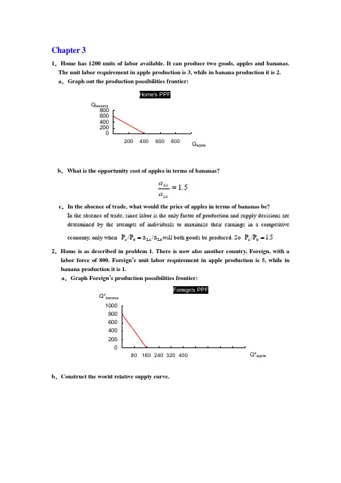
Chapter 31．Home has 1200 units of labor available. It can produce two goods, apples and bananas. The unit labor requirement in apple production is 3, while in banana production it is 2. a ．Graph out the production possibilities frontier:b ．What is the opportunity cost of apples in terms of bananas?5.1=LbLa a a c ．In the absence of trade, what would the price of apples in terms of bananas be?In the absence of trade, since labor is the only factor of production and supply decisions aredetermined by the attempts of individuals to maximize their earnings in a competitive economy, only when Lb La b a /a a /P P =will both goods be produced. So 1.5 /P P b a =2．Home is as described in problem 1. There is now also another country, Foreign, with alabor force of 800. Foreign ’s unit labor requirement in apple production is 5, while in banana production it is 1.a ．Graph Foreign ’s production possibilities frontier:b ．Construct the world relative supply curve.Home's PPF 0200400600800200400600800Q apple Q banana Foreign's PPF0200400600800100080160240320400Q*apple Q*banana3．Now suppose world relative demand takes the following form: Demand for apples/demandfor bananas = price of bananas/price of apples.a ．Graph the relative demand curve along with the relative supply curve:a b b a /P P /D D =∵When the market achieves its equilibrium, we have 1b a )(D D -**=++=ba b b a a P P Q Q Q Q ∴RD is a hyperbola xy 1=b ．What is the equilibrium relative price of apples?The equilibrium relative price of apples is determined by the intersection of the RD and RScurves.RD: yx 1= RS: 5]5,5.1[5.1],5.0(5.0)5.0,0[=∈=⎪⎩⎪⎨⎧+∞∈=∈y y y x x x ∴25.0==y x∴2/=b P a P e ec ．Describe the pattern of trade.∵b a b e a e b a P P P P P P ///>>**∴In this two-country world, Home will specialize in the apple production, export apples and import bananas. Foreign will specialize in the banana production, export bananas and import apples.d ．Show that both Home and Foreign gain from trade.International trade allows Home and Foreign to consume anywhere within the coloredlines, which lie outside the countries ’ production possibility frontiers. And the indirect method, specializing in producing only one production then trade with other country, is a more efficient method than direct production. In the absence of trade, Home could gain three bananas by foregoing two apples, and Foreign could gain by one foregoing five bananas. Trade allows each country to trade two bananas for one apple. Home could then gain four bananas by foregoing two apples while Foreign could gain one apple by foregoing only two bananas. So both Home and Foreign gain from trade.4．Suppose that instead of 1200 workers, Home had 2400. Find the equilibrium relative price. What can you say about the efficiency of world production and the division of the gains from trade between Home and Foreign in this case?RD: yx 1= RS: 5]5,5.1[5.1],1(1)1,0[=∈=⎪⎩⎪⎨⎧+∞∈=∈y y y x x x ∴5.132==y x ∴5.1/=b P a P e eIn this case, Foreign will specialize in the banana production, export bananas and import apples. But Home will produce bananas and apples at the same time. And the opportunity cost of bananas in terms of apples for Home remains the same. So Home neither gains nor loses but Foreign gains from trade.5．Suppose that Home has 2400 workers, but they are only half as production in both industries as we have been assuming, Construct the world relative supply curve and determine the equilibrium relative price. How do the gains from trade compare with those in the case described in problem 4?In this case, the labor is doubled while the productivity of labor is halved, so the ＂effective labor＂remains the same. So the answer is similar to that in 3. And both Home and Foreign can gain from trade. But Foreign gains lesser compare with that in the case 4.6．”Korean workers earn only $ an hour; if we allow Korea to export as much as it likes to the United States, our workers will be forced down to the same level. You can’t import a $5 shirt without importing the $ wage that goes with it.” Discuss.In fact, relative wage rate is determined by comparative productivity and the relative demand for goods. Korea’s low wage reflects the fact that Korea is less productive than the United States in most industries. Actually, trade with a less productive, low wage country can raise the welfare and standard of living of countries with high productivity, such as United States. Sothis pauper labor argument is wrong.7．Japanese labor productivity is roughly the same as that of the United States in the manufacturing sector (higher in some industries, lower in others), while the United States, is still considerably more productive in the service sector. But most services are non-traded. Some analysts have argued that this poses a problem for the United States, because our comparative advantage lies in things we cannot sell on world markets. What is wrong with this argument?The competitive advantage of any industry depends on both the relative productivities of the industries and the relative wages across industries. So there are four aspects should be taken into account before we reach conclusion: both the industries and service sectors of Japan and U.S., not just the two service sectors. So this statement does not bade on the reasonable logic. 8．Anyone who has visited Japan knows it is an incredibly expensive place; although Japanese workers earn about the same as their . counterparts, the purchasing power of their incomes is about one-third less. Extend your discussing from question 7 to explain this observation. (Hint: Think about wages and the implied prices of non-trade goods.) The relative higher purchasing power of U.S. is sustained and maintained by its considerably higher productivity in services. Because most of those services are non-traded, Japanese could not benefit from those lower service costs. And U.S. does not have to face a lower international price of services. So the purchasing power of Japanese is just one-third of their U.S. counterparts.9．How does the fact that many goods are non-traded affect the extent of possible gains from trade?Actually the gains from trade depended on the proportion of non-traded goods. The gains will increase as the proportion of non-traded goods decrease.10．We have focused on the case of trade involving only two countries. Suppose that there are many countries capable of producing two goods, and that each country has only one factor of production, labor. What could we say about the pattern of production and in this case? (Hint: Try constructing the world relative supply curve.)Any countries to the left of the intersection of the relative demand and relative supply curves export the good in which they have a comparative advantage relative to any country to the right of the intersection. If the intersection occurs in a horizontal portion then the country with that price ratio produces both goods.Chapter 41． In the United States where land is cheap, the ratio of land to labor used in cattle rising ishigher than that of land used in wheat growing. But in more crowded countries, where land is expensive and labor is cheap, it is common to raise cows by using less land and more labor than Americans use to grow wheat. Can we still say that raising cattle is land intensive compared with farming wheat? Why or why not?The definition of cattle growing as land intensive depends on the ratio of land to labor used inproduction, not on the ratio of land or labor to output. The ratio of land to labor in cattle exceeds the ratio in wheat in the United States, implying cattle is land intensive in the United States. Cattle is land intensive in other countries too if the ratio of land to labor in cattle production exceeds the ratio in wheat production in that country. The comparison between another country and the United States is less relevant for answering the question.2． Suppose that at current factor prices cloth is produced using 20 hours of labor for eachacre of land, and food is produced using only 5 hours of labor per acre of land.a. Suppose that the economy ’s total resources are 600 hours of labor and 60 acres ofland. Using a diagram determine the allocation of resources.5TF LF /TF LF /QF)(TF / /QF)(LF aTF / aLF 20TC LC /TC LC /QC)(TC / /QC)(LC aTC / aLC =⇒===⇒==We can solve this algebraically since L=LC+LF=600 and T=TC+TF=60. The solution is LC=400, TC=20, LF=200 and TF=40.b. Now suppose that the labor supply increase first to 800, then 1000, then 1200 hours. Using a diagram like Figure4-6, trace out the changing allocation of resources. Labor Land ClothFoodLCLF TCTFtion).specializa (complete 0.LF 0,TF 1200,LC 60,TC :1200L 66.67LF 13.33,TF 933.33,LC 46.67,TC :1000L 133.33LF 26.67,TF 666.67,LC 33.33,TC :800L ===============c. What would happen if the labor supply were to increase even further?At constant factor prices, some labor would be unused, so factor prices would have tochange, or there would be unemployment.3. “The world ’s poorest countries cannot find anything to export. There is no resource thatis abundant — certainly not capital or land, and in small poor nations not even labor is abundant.” Discuss.The gains from trade depend on comparative rather than absolute advantage. As to poor countries, what matters is not the absolute abundance of factors, but their relative abundance. Poor countries have an abundance of labor relative to capital when compared to more developed countries.4. The U.S. labor movement — which mostly represents blue-collar workers rather thanprofessionals and highly educated workers — has traditionally favored limits on imports form less-affluent countries. Is this a shortsighted policy of a rational one in view of the interests of union members? How does the answer depend on the model of trade?In the Ricardo ’s model, labor gains from trade through an increase in its purchasing power. This result does not support labor union demands for limits on imports from less affluent countries.In the Immobile Factors model labor may gain or lose from trade. Purchasing power in terms of one good will rise, but in terms of the other good it will decline.The Heckscher-Ohlin model directly discusses distribution by considering the effects of trade on the owners of factors of production. In the context of this model, unskilled U.S. labor loses from trade since this group represents the relatively scarce factors in this country. The results from the Heckscher-Ohlin model support labor union demands for import limits. 5. There is substantial inequality of wage levels between regions within the United States. Labor Land Cloth Food0l 800 0l 1000 0l 1200For example, wages of manufacturing workers in equivalent jobs are about 20 percent lower in the Southeast than they are in the Far West. Which of the explanations of failure of factor price equalization might account for this? How is this case different from the divergence of wages between the United States and Mexico (which is geographically closer to both the . Southeast and the Far West than the Southeast and Far West are to each other)?When we employ factor price equalization, we should pay attention to its conditions: both countries/regions produce both goods; both countries have the same technology of production, and the absence of barriers to trade. Inequality of wage levels between regions within the United States may caused by some or all of these reasons.Actually, the barriers to trade always exist in the real world due to transportation costs. And the trade between U.S. and Mexico, by contrast, is subject to legal limits; together with cultural differences that inhibit the flow of technology, this may explain why the difference in wage rates is so much larger.6.Explain why the Leontief paradox and the more recent Bowen, Leamer, andSveikauskas results reported in the text contradict the factor-proportions theory.The factor proportions theory states that countries export those goods whose production is intensive in factors with which they are abundantly endowed. One would expect the United States, which has a high capital/labor ratio relative to the rest of the world, to export capital-intensive goods if the Heckscher-Ohlin theory holds. Leontief found that the United States exported labor-intensive goods. Bowen, Leamer and Sveikauskas found that the correlation between factor endowment and trade patterns is weak for the world as a whole.The data do not support the predictions of the theory that countries' exports and imports reflect the relative endowments of factors.7.In the discussion of empirical results on the Heckscher-Ohlin model, we noted thatrecent work suggests that the efficiency of factors of production seems to differ internationally. Explain how this would affect the concept of factor price equalization.If the efficiency of the factors of production differs internationally, the lessons of the Heckscher-Ohlin theory would be applied to “effective factors” which adjust for the differences in technology or worker skills or land quality (for example). The adjusted model has been found to be more successful than the unadjusted model at explaining the pattern of trade between countries. Factor-price equalization concepts would apply to the effective factors. A worker with more skills or in a country with better technology could be considered to be equal to two workers in another country. Thus, the single person would be two effective units of labor. Thus, the one high-skilled worker could earn twice what lower skilled workers do and the price of one effective unit of labor would still be equalized.chapter 81. The import demand equation, MD, is found by subtracting the home supply equation from the home demand equation. This results in MD = 80 - 40 x P. Without trade, domestic prices and quantities adjust such that import demand is zero. Thus, the price in the absence of trade is2.2. a. Foreign's export supply curve, XS, is XS = -40 + 40 x P. In the absence of trade, the price is 1.b. When trade occurs export supply is equal to import demand, XS = MD. Thus, using theequations from problems 1 and 2a, P = , and the volume of trade is 20.3. a. The new MD curve is 80 - 40 x (P+t) where t is the specific tariff rate, equal to . (Note: in solving these problems you should be careful about whether a specific tariff or ad valorem tariff is imposed. With an ad valorem tariff, the MD equation would be expressed as MD =80-40 x (1+t)P). The equation for the export supply curve by the foreign country is unchanged. Solving, we find that the world price is $, and thus the internal price at home is $. The volume of trade has been reduced to 10, and the total demand for wheat at home has fallen to 65 (from the free trade level of70). The total demand for wheat in Foreign has gone up from 50 to 55.b. andc. The welfare of the home country is best studied using the combined numerical andgraphical solutions presented below in Figure 8-1. Home SupplyHome Demanda b c d e P T =1.7550556070QuantityPrice P W =1.50P T*=1.25where the areas in the figure are:a: 55 (55-50) .5(55-50) (65-55) .5(70-65) (65-55) surplus change: -(a+b+c+d)=. Producer surplus change: a=. Government revenue change: c+e=5. Efficiency losses b+d are exceeded by terms of trade gain e. [Note: in the calculations for the a, b, and d areas a figure of .5 shows up. This is because we are measuring the area of a triangle, which is one-half of the area of the rectangle defined by the product of the horizontal and vertical sides.]4. Using the same solution methodology as in problem 3, when the home country is very small relative to the foreign country, its effects on the terms of trade are expected to be much less. The small country is much more likely to be hurt by its imposition of a tariff. Indeed, this intuition is shown in this problem. The free trade equilibrium is now at the price $ and the trade volume is now $.With the imposition of a tariff of by Home, the new world price is $, the internal home price is $, home demand is units, home supply is and the volume of trade is . When Home is relatively small, the effect of a tariff on world price is smaller than when Home is relatively large. When Foreign and Home were closer in size, a tariff of .5 by home lowered world price by 25 percent, whereas in this case the same tariff lowers world price by about 5 percent. The internal Home price is now closer to the free trade price plus t than when Home was relatively large. In this case, the government revenues from the tariff equal , the consumer surplus loss is , and the producer surplus gain is . The distortionary losses associated with the tariff (areas b+d) sum to and the terms of trade gain (e) is . Clearly, in this small country example the distortionary losses from the tariff swamp the terms of trade gains. The general lesson is the smaller the economy,the larger the losses from a tariff since the terms of trade gains are smaller.5. The effective rate of protection takes into consideration the costs of imported intermediate goods. In this example, half of the cost of an aircraft represents components purchased from other countries. Without the subsidy the aircraft would cost $60 million. The European value added to the aircraft is $30 million. The subsidy cuts the cost of the value added to purchasers of the airplane to $20 million. Thus, the effective rate of protection is (30 - 20)/20 = 50%.6. We first use the foreign export supply and domestic import demand curves to determine the new world price. The foreign supply of exports curve, with a foreign subsidy of 50 percent per unit, becomes XS = -40 + 40(1+ x P. The equilibrium world price is and the internal foreign price is . The volume of trade is 32. The foreign demand and supply curves are used to determine the costs and benefits of the subsidy. Construct a diagram similar to that in the text and calculate the area of the various polygons. The government must provide - x 32 = units of output to support the subsidy. Foreign producers surplus rises due to the subsidy by the amount of units of output. Foreign consumers surplus falls due to the higher price by units of the good. Thus, the net loss to Foreign due to the subsidy is + - = units of output. Home consumers and producers face an internal price of as a result of the subsidy. Home consumers surplus rises by 70 x .3 + .5 (6= while Home producers surplus falls by 44 x .3 + .5(6 x .3) = , for a net gain of units of output.7. At a price of $10 per bag of peanuts, Acirema imports 200 bags of peanuts. A quota limiting the import of peanuts to 50 bags has the following effects:a. The price of peanuts rises to $20 per bag.b. The quota rents are ($20 - $10) x 50 = $500.c. The consumption distortion loss is .5 x 100 bags x $10 per bag = $500.d. The production distortion loss is .5 x50 bags x$10 per bag = $250.。