matlab-线性分类器的设计doc
6-线性分类器设计-第六章

k 此法可收敛于W值。W满足: XT(XW-b)=0
令 ρk =
ρ1
其中 ρ 1 为任意常数
因此下降算法不论XTX是否奇异,总能产生一个解。 若训练样本无限的重复出现,则简化为 W1任意 Wk+1=Wk+ρk(bk-WkTXk) Xk k+1
取 ρK
=
ρ1
k
ρk随迭代次数k而减少,以保证算法收敛于满意的W值
其中N/N1有N1个,N/N2有N2个
四 韦—霍氏法(LMS法)迭代法
上节得到MSE法的W解为:W=X+b
伪逆 X + =
(
XT X
)
−1
X
T
计算量很大
在计算X+时, 1. 要求XTX矩阵为非奇异 2 2. 由于计算量太大而引入比较大误差 所以要用迭代法来求 求J(W)的梯度 ▽J(W) =2XT(XW-b) 代入迭代公式 W1任意设定 Wk+1 = Wk-ρkXT(XWk-b)
H wk+1 ρk x
权值修正过程
例题:有两类样本 ω1=(x1,x2)={(1,0,1),(0,1,1)} ω2=(x3,x4)={(1,1,0),(0,1,0)} 解:先求四个样本的增值模式 x1=(1,0,1,1) x2=(0,1,1,1) x3=(1,1,0,1) x4=(0,1,0,1) 假设初始权向量 w1=(1,1,1,1) ρk=1 第一次迭代: w1Tx1=(1,1,1,1) (1,0,1,1)T=3>0 所以不修正 w1Tx2=(1,1,1,1) (0,1,1,1)T=3>0 所以不修正 w1Tx3=(1,1,1,1) (1,1,0,1)T=3>0 所以修正w1 w2=w1-x3=(0,0,1,0) w2Tx4=(0,0,1,0)T (0,1,0,1) =0 所以修正w2 w3=w2-x4=(0,-1,1,-1) 第一次迭代后,权向量w3=(0,-1,1,-1),再进行第2,3,…次迭代 如下表
Matlab的SVM算法进行线性和非线性分类实例_20131128

Matlab_svmtranin_example1.Linear classification%Two Dimension Linear-SVM Problem,Two Class and Separable Situation%Method from Christopher J.C.Burges:%"A Tutorial on Support Vector Machines for Pattern Recognition",page9 %Optimizing||W||directly:%Objective:min"f(A)=||W||",p8/line26%Subject to:yi*(xi*W+b)-1>=0,function(12);clear all;close allclc;sp=[3,7;6,6;4,6;5,6.5]%positive sample pointsnsp=size(sp);sn=[1,2;3,5;7,3;3,4;6,2.7]%negative sample pointsnsn=size(sn)sd=[sp;sn]lsd=[true true true true false false false false false]Y=nominal(lsd)figure(1);subplot(1,2,1)plot(sp(1:nsp,1),sp(1:nsp,2),'m+');hold onplot(sn(1:nsn,1),sn(1:nsn,2),'c*');subplot(1,2,2)svmStruct=svmtrain(sd,Y,'showplot',true);2.NonLinear classification%Two Dimension quadratic-SVM Problem,Two Class and Separable Situation %Method from Christopher J.C.Burges:%"A Tutorial on Support Vector Machines for Pattern Recognition",page9 %Optimizing||W||directly:%Objective:min"f(A)=||W||",p8/line26%Subject to:yi*(xi*W+b)-1>=0,function(12);clear all;close allclc;sp=[3,7;6,6;4,6;5,6.5]%positive sample pointsnsp=size(sp);sn=[1,2;3,5;7,3;3,4;6,2.7;4,3;2,7]%negative sample pointsnsn=size(sn)sd=[sp;sn]lsd=[true true true true false false false false false false false]Y=nominal(lsd)figure(1);subplot(1,2,1)plot(sp(1:nsp,1),sp(1:nsp,2),'m+');hold onplot(sn(1:nsn,1),sn(1:nsn,2),'c*');subplot(1,2,2)%svmStruct=svmtrain(sd,Y,'Kernel_Function','linear','showplot',true);svmStruct=svmtrain(sd,Y,'Kernel_Function','quadratic','showplot',true);%use the trained svm(svmStruct)to classify the dataRD=svmclassify(svmStruct,sd,'showplot',true)%RD is the classification result vector3.Svmtrainsvmtrain Train a support vector machine classifierSVMSTRUCT=svmtrain(TRAINING,Y)trains a support vector machine(SVM) classifier on data taken from two groups.TRAINING is a numeric matrix of predictor data.Rows of TRAINING correspond to observations;columns correspond to features.Y is a column vector that contains the knownclass labels for TRAINING.Y is a grouping variable,i.e.,it can be a categorical,numeric,or logical vector;a cell vector of strings;or a character matrix with each row representing a class label(see help forgroupingvariable).Each element of Y specifies the group thecorresponding row of TRAINING belongs to.TRAINING and Y must have the same number of rows.SVMSTRUCT contains information about the trained classifier,including the support vectors,that is used by SVMCLASSIFY for classification.svmtrain treats NaNs,empty strings or'undefined' values as missing values and ignores the corresponding rows inTRAINING and Y.SVMSTRUCT=svmtrain(TRAINING,Y,'PARAM1',val1,'PARAM2',val2,...) specifies one or more of the following name/value pairs:Name Value'kernel_function'A string or a function handle specifying thekernel function used to represent the dotproduct in a new space.The value can be one ofthe following:'linear'-Linear kernel or dot product(default).In this case,svmtrainfinds the optimal separating planein the original space.'quadratic'-Quadratic kernel'polynomial'-Polynomial kernel with defaultorder3.To specify another order,use the'polyorder'argument.'rbf'-Gaussian Radial Basis Functionwith default scaling factor1.Tospecify another scaling factor,use the'rbf_sigma'argument.'mlp'-Multilayer Perceptron kernel(MLP)with default weight1and defaultbias-1.To specify another weightor bias,use the'mlp_params'argument.function-A kernel function specified using@(for example@KFUN),or ananonymous function.A kernelfunction must be of the formfunction K=KFUN(U,V)The returned value,K,is a matrixof size M-by-N,where M and N arethe number of rows in U and Vrespectively.'rbf_sigma'A positive number specifying the scaling factorin the Gaussian radial basis function kernel.Default is1.'polyorder'A positive integer specifying the order of thepolynomial kernel.Default is3.'mlp_params'A vector[P1P2]specifying the parameters of MLPkernel.The MLP kernel takes the form:K=tanh(P1*U*V'+P2),where P1>0and P2<0.Default is[1,-1].'method'A string specifying the method used to find theseparating hyperplane.Choices are:'SMO'-Sequential Minimal Optimization(SMO)method(default).It implements the L1soft-margin SVM classifier.'QP'-Quadratic programming(requires anOptimization Toolbox license).Itimplements the L2soft-margin SVMclassifier.Method'QP'doesn't scalewell for TRAINING with large number ofobservations.'LS'-Least-squares method.It implements theL2soft-margin SVM classifier.'options'Options structure created using either STATSET orOPTIMSET.*When you set'method'to'SMO'(default),create the options structure using STATSET.Applicable options:'Display'Level of display output.Choicesare'off'(the default),'iter',and'final'.Value'iter'reports every500iterations.'MaxIter'A positive integer specifying themaximum number of iterations allowed.Default is15000for method'SMO'.*When you set method to'QP',create theoptions structure using OPTIMSET.For detailsof applicable options choices,see QUADPROGoptions.SVM uses a convex quadratic program,so you can choose the'interior-point-convex'algorithm in QUADPROG.'tolkkt'A positive scalar that specifies the tolerancewith which the Karush-Kuhn-Tucker(KKT)conditionsare checked for method'SMO'.Default is1.0000e-003.'kktviolationlevel'A scalar specifying the fraction of observationsthat are allowed to violate the KKT conditions formethod'SMO'.Setting this value to be positivehelps the algorithm to converge faster if it isfluctuating near a good solution.Default is0.'kernelcachelimit'A positive scalar S specifying the size of thekernel matrix cache for method'SMO'.Thealgorithm keeps a matrix with up to S*Sdouble-precision numbers in memory.Default is5000.When the number of points in TRAININGexceeds S,the SMO method slows down.It'srecommended to set S as large as your systempermits.'boxconstraint'The box constraint C for the soft margin.C can bea positive numeric scalar or a vector of positivenumbers with the number of elements equal to thenumber of rows in TRAINING.Default is1.*If C is a scalar,it is automatically rescaledby N/(2*N1)for the observations of group one,and by N/(2*N2)for the observations of grouptwo,where N1is the number of observations ingroup one,N2is the number of observations ingroup two.The rescaling is done to take intoaccount unbalanced groups,i.e.,when N1and N2are different.*If C is a vector,then each element of Cspecifies the box constraint for thecorresponding observation.'autoscale'A logical value specifying whether or not toshift and scale the data points before training.When the value is true,the columns of TRAININGare shifted and scaled to have zero mean unitvariance.Default is true.'showplot'A logical value specifying whether or not to showa plot.When the value is true,svmtrain creates aplot of the grouped data and the separating linefor the classifier,when using data with2features(columns).Default is false. SVMSTRUCT is a structure having the following properties:SupportVectors Matrix of data points with each row correspondingto a support vector.Note:when'autoscale'is false,this fieldcontains original support vectors in TRAINING.When'autoscale'is true,this field containsshifted and scaled vectors from TRAINING.Alpha Vector of Lagrange multipliers for the supportvectors.The sign is positive for support vectorsbelonging to the first group and negative forsupport vectors belonging to the second group. Bias Intercept of the hyperplane that separatesthe two groups.Note:when'autoscale'is false,this fieldcorresponds to the original data points inTRAINING.When'autoscale'is true,this fieldcorresponds to shifted and scaled data points. KernelFunction The function handle of kernel function used. KernelFunctionArgs Cell array containing the additional argumentsfor the kernel function.GroupNames A column vector that contains the knownclass labels for TRAINING.Y is a groupingvariable(see help for groupingvariable). SupportVectorIndices A column vector indicating the indices of supportvectors.ScaleData This field contains information about auto-scale.When'autoscale'is false,it is empty.When'autoscale'is set to true,it is a structurecontaining two fields:shift-A row vector containing the negativeof the mean across all observationsin TRAINING.scaleFactor-A row vector whose value is1./STD(TRAINING).FigureHandles A vector of figure handles created by svmtrainwhen'showplot'argument is TRUE.Example:%Load the data and select features for classificationload fisheririsX=[meas(:,1),meas(:,2)];%Extract the Setosa classY=nominal(ismember(species,'setosa'));%Randomly partitions observations into a training set and a test %set using stratified holdoutP=cvpartition(Y,'Holdout',0.20);%Use a linear support vector machine classifiersvmStruct=svmtrain(X(P.training,:),Y(P.training),'showplot',true);C=svmclassify(svmStruct,X(P.test,:),'showplot',true);errRate=sum(Y(P.test)~=C)/P.TestSize%mis-classification rate conMat=confusionmat(Y(P.test),C)%the confusion matrix。
作业2-线性分类器
end; for i=1:N1 x(1,i)=x1(1,i); x(2,i)=x1(2,i); y(i)=1; end; for i=(N1+1):(N1+N2) x(1,i)=x2(1,(i-N1)); x(2,i)=x2(2,(i-N1)); y(i)=-1; end; svm_struct=svmtrain(x,y,'Showplot',true); % 调用 svmtrain 函数对样本进行分类 % 分别创建训练样本矩阵和标号矩阵
x1(1,i)=-1.7+1.1*randn(1); x1(2,i)= 1.6+0.9*randn(1); x1(3,i)= 1; end; N2=400; for i=1:N2 x2(1,i)= 1.3+1.0*randn(1); x2(2,i)=-1.5+0.8*randn(1); x2(3,i)= 1; % 2 类400个训练样本,2维正态分布 % 1 类440个训练样本,2维正态分布
算法 2.
w(1)=rand(1); %对w 赋任意初值 w(2)=rand(1); w(3)=rand(1); p=0.001; %设置步长大小,一般在0~1 之间取值 for j=1:100 %j 为迭代次数,共迭代100 次 k=0; %k 是记录两类的样本误分类点的次数 n(j)=j; %n 记录迭代次数 for i=1:N1 xe=x1(:,i); %将1 类的各个样本值取出来,存入xe 中 if(w*xe<0) %1 类的迭代修正判断条件 w=w+p*xe'; %1 类的迭代修正公式,每次只修正一个样本的 %固定增量法 k=k+1; %记录1 类的误分类点总次数 end; end; for i=1:N2 xe=x2(:,i); %将2 类的各个样本值取出来,存入xe 中 if(w*xe>0) %2 类的迭代修正判断条件 w=w-p*xe'; %2 类的迭代修正公式,每次只修正一个样本的 %固定增量法 k=k+1; %记录1、2 类的误分类点总次数 end; end; en(j)=k; %en 记录每一次迭代中误分类点总次数 end; subplot(2,2,1); plot(n,en); %画图,横坐标为迭代次数,纵坐标为每次迭代 的误分类点总次数画图 t1=-5:1:5; %t1 范围是-5~5,步长为1 t2=(-w(1)*t1-w(3))/w(2); %求决策面 subplot(2,2,2);
3种线性分类器的设计及MATLAB建模
x1(38,1)=4.1025; x1(38,2)=4.4063; x1(39,1)=3.9590; x1(39,2)=1.3024; x1(40,1)=1.7524; x1(40,2)=1.9339; x1(41,1)=3.4892; x1(41,2)=1.2457; x1(42,1)=4.2492; x1(42,2)=4.5982; x1(43,1)=4.3692; x1(43,2)=1.9794; x1(44,1)=4.1792; x1(44,2)=0.4113; x1(45,1)=3.9627; x1(45,2)=4.2198;
for i=1:45 r1(i)=x1(i,1);end; for i=1:45 r2(i)=x1(i,2);end; for i=1:55 r3(i)=x2(i,1);end; for i=1:55 r4(i)=x2(i,2);end; figure(1);
plot(r1,r2,'*',r3,r4,'o'); hold on;%保持当前的轴和图像不被刷新,在该图上接着绘制下一图 x1(:,3) = 1;% 考虑到不经过原点的超平面,对x进行扩维 x2(:,3) = 1;% 使x'=[x 1],x为2维的,故加1扩为3维 %进行初始化
w = rand(3,1);% 随机给选择向量,生成一个3维列向量 p = 1; %p0非负正实数 ox1 = -1;% 代价函数中的变量
x2(1,1)=9.7302; x2(1,2)=5.5080; x2(2,1)=8.8067; x2(2,2)=5.1319; x2(3,1)=8.1664; x2(3,2)=5.2801; x2(4,1)=6.9686; x2(4,2)=4.0172; x2(5,1)=7.0973; x2(5,2)=4.0559; x2(6,1)=9.4755; x2(6,2)=4.9869; x2(7,1)=9.3809; x2(7,2)=5.3543; x2(8,1)=7.2704; x2(8,2)=4.1053; x2(9,1)=8.9674; x2(9,2)=5.8121; x2(10,1)=8.2606; x2(10,2)=5.1095; x2(11,1)=7.5518; x2(11,2)=7.7316; x2(12,1)=7.0016; x2(12,2)=5.4111; x2(13,1)=8.3442; x2(13,2)=3.6931; x2(14,1)=5.8173; x2(14,2)=5.3838; x2(15,1)=6.1123; x2(15,2)=5.4995; x2(17,1)=7.9136; x2(17,2)=5.2349; x2(19,1)=7.7080; x2(19,2)=5.0208; x2(20,1)=8.2079; x2(20,2)=5.4194; x2(21,1)=9.1078; x2(21,2)=6.1911; x2(22,1)=7.7857; x2(22,2)=5.7712; x2(23,1)=7.3740; x2(23,2)=2.3558; x2(24,1)=9.7184; x2(24,2)=5.2854; x2(25,1)=6.9559; x2(25,2)=5.8261; x2(26,1)=8.9691; x2(26,2)=4.9919; x2(27,1)=7.3872; x2(27,2)=5.8584; x2(28,1)=8.8922; x2(28,2)=5.7748; x2(29,1)=9.0175; x2(29,2)=6.3059; x2(30,1)=7.0041; x2(30,2)=6.2315; x2(31,1)=8.6396; x2(31,2)=5.9586; x2(32,1)=9.2394; x2(32,2)=3.3455; x2(33,1)=6.7376; x2(33,2)=4.0096; x2(34,1)=8.4345; x2(34,2)=5.6852; x2(16,1)=10.4188; x2(16,2)=4.4892; x2(18,1)=11.1547; x2(18,2)=4.4022;
矩阵计算-MATLAB-利用最小二乘法生成一个线性分类器

hold;
plot(x2,y2);些离散的点
四、心得体会
通过本次实验我熟悉线性分类器的概念,了解有哪些主流的分类器,并且通过对现有知识的学习,我会利用最小二乘法设计一个线性分类器。首先在实验前,应该先了解最先二乘法和线性分类器的概念,这样以便于我们做实验。本次实验是基于一次函数y=kx+b形式进行实验的,在实验时,我先求出了系数k和截距b。在做实验时,要先利用程序代码生成一些离散的点,其次要利用程序对离散点进行曲线拟合。本次实验也或多或少的出现了一些问题,比如:开始时,不知道散点图怎么绘制,曲线怎么拟合,好在自己查阅资料,一点点的解决了。
B(1,1)=B(1,1)+x(i)*y(i);
B(2,1)=B(2,1)+y(i);
end
A(2,1)=A(1,2);
S=A\B;
a=S(1);
b=S(2);
end
2)在command windows窗口中输入以下代码
[a,b]=OnePolyFit(x,y)%直线一次拟合,生成拟合后图像
x2=linspace(0,10);
x1=linspace(0,10);
y1=x1+0.28;
plot(x1,y1);%生成仿真测量数据
x=linspace(0,10,30);
y=x+0.28+0.1*randn(1,length(x))
plot(x,y,'ro');%显示测量数据
2、对形如y=kx+b曲线拟合。
1)建立M文件
function [a,b]=OnePolyFit(x,y)%线性拟合函数
姓名学号专业班级
课程名称矩阵分析与计算实验名称利用最小二乘法生成一个线性分类器
matlab-线性分类器的设计doc

线性分类器设计1 问题描述对“data1.m ”数据,分别采用感知机算法、最小平方误差算法、线性SVM 算法设计分类器,分别画出决策面,并比较性能。
(注意讨论算法中参数设置的影响。
)2 方法描述2.1 感知机算法线性分类器的第一个迭代算法是1956年由Frank Rosenblatt 提出的,即具有自学习能力的感知器(Perceptron )神经网络模型,用来模拟动物或者人脑的感知和学习能力。
这个算法被提出后,受到了很大的关注。
感知器在神经网络发展的历史上占据着特殊的位置:它是第一个从算法上完整描述的神经网络,是一种具有分层神经网络结构、神经元之间有自适应权相连接的神经网络的一个基本网络。
感知器的学习过程是不断改变权向量的输入,更新结构中的可变参数,最后实现在有限次迭代之后的收敛。
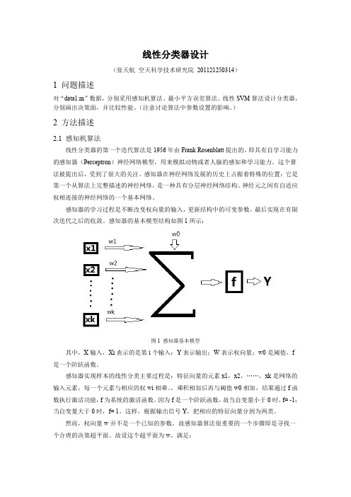
感知器的基本模型结构如图1所示:图1 感知器基本模型其中,X 输入,Xi 表示的是第i 个输入;Y 表示输出;W 表示权向量;w0是阈值,f 是一个阶跃函数。
感知器实现样本的线性分类主要过程是:特征向量的元素x1,x2,……,xk 是网络的输入元素,每一个元素与相应的权wi 相乘。
,乘积相加后再与阈值w0相加,结果通过f 函数执行激活功能,f 为系统的激活函数。
因为f 是一个阶跃函数,故当自变量小于0时,f= -1;当自变量大于0时,f= 1。
这样,根据输出信号Y ,把相应的特征向量分到为两类。
然而,权向量w 并不是一个已知的参数,故感知器算法很重要的一个步骤即是寻找一个合理的决策超平面。
故设这个超平面为w ,满足:12*0,*0,T Tw x x w x x ωω>∀∈<∀∈ (1)引入一个代价函数,定义为:()**T x x YJ w w xδ∈=∑ (2)其中,Y 是权向量w 定义的超平面错误分类的训练向量的子集。
变量x δ定义为:当1x ω∈时,x δ= -1;当2x ω∈时,x δ= +1。
显然,J(w)≥0。
MATLAB线性系统
y (t ) Cx(t )
利用状态反馈U(t)= - KX(t)+r(t) 其中K为状态反馈 矩阵, r(t)为参考输入,
r
u
B
x
A
x
C
y
k
(t ) ( A BK )x(t ) Br (t ) 使得系统闭环方程为: x y (C DK )x(t )
几个常用命令 M=ctrb(A,B) 系统的能控矩阵 M=[B AB A2B … An-1B] rank(M) 得到矩阵的秩,M的秩为n,则能控 N=obsv(A,C) 求取系统的能观矩阵 N=[C CA CA2 … CAn-1]T, N的秩为n,则能观 二、单输入系统的极点配置 k=acker(A,B,p) 对于期望极点p,求出系统的状态反 馈增益阵k
传递函数使用分子、分母的多项式表示,即num和 den两个向量。
同样可用SYS = TF(NUM,DEN)建立tf模型。
num=[1 2 3]; den=[2 2 3 4]; yy=tf(num,den)
Transfer function: s^2 + 2 s + 3 ----------------------2 s^3 + 2 s^2 + 3 s + 4
f1=ss(a,b,c,d,0.1)
a = x1 x2 x1 1 2 x2 3 4 c = x1 x2 y1 1 1 b = u1 x1 0 x2 1 d = u1 y1 1
x2 x1 1 2 x2 3 4 c = x1 x2 y1 1 1
b = u1 x1 0 x2 1 d = u1 y1 1
Continuous-time model.
step(sys,t) [y,t,x]=step(sys)
matlab线性规划课程设计
matlab线性规划课程设计一、课程目标知识目标:1. 学生能理解线性规划的基本概念,掌握线性规划问题的数学模型及其应用;2. 学生能运用MATLAB软件进行线性规划问题的建模与求解;3. 学生能掌握线性规划问题求解过程中涉及的矩阵运算和算法原理。
技能目标:1. 学生能运用MATLAB软件构建线性规划模型,并进行有效求解;2. 学生能通过实例分析,学会运用线性规划方法解决实际问题;3. 学生能运用所学的知识,对线性规划问题进行优化和改进。
情感态度价值观目标:1. 学生培养对线性规划问题的兴趣,提高解决实际问题的热情;2. 学生培养团队协作意识,学会与他人共同探讨和分析问题;3. 学生通过解决线性规划问题,认识到数学工具在现代科技发展中的重要性。
课程性质:本课程为应用数学课程,旨在培养学生运用MATLAB软件解决线性规划问题的能力。
学生特点:学生具备一定的数学基础,对计算机软件操作有一定了解,但可能对线性规划及其应用尚不熟悉。
教学要求:结合学生特点,注重理论与实践相结合,通过实例教学,使学生在掌握线性规划基本知识的同时,提高实际操作能力。
将课程目标分解为具体的学习成果,便于后续教学设计和评估。
二、教学内容1. 线性规划基本概念:线性规划问题的数学模型、线性约束条件、目标函数、可行解和最优解。
2. MATLAB软件操作:MATLAB基本操作、矩阵运算、函数调用、数据可视化。
3. 线性规划建模与求解:线性规划问题的建模方法、单纯形法、内点法、MATLAB求解线性规划问题的函数。
4. 实例分析:经济管理中的线性规划问题、生产计划问题、运输问题、分配问题。
5. 线性规划优化:线性规划问题的灵敏度分析、对偶问题、参数优化。
教学大纲安排:第一周:线性规划基本概念,MATLAB软件入门;第二周:线性规划建模方法,MATLAB矩阵运算;第三周:单纯形法与内点法,MATLAB求解线性规划问题;第四周:实例分析,探讨线性规划在实际问题中的应用;第五周:线性规划优化,灵敏度分析与对偶问题。
- 1、下载文档前请自行甄别文档内容的完整性,平台不提供额外的编辑、内容补充、找答案等附加服务。
- 2、"仅部分预览"的文档,不可在线预览部分如存在完整性等问题,可反馈申请退款(可完整预览的文档不适用该条件!)。
- 3、如文档侵犯您的权益,请联系客服反馈,我们会尽快为您处理(人工客服工作时间:9:00-18:30)。
线性分类器设计1 问题描述对“data1.m ”数据,分别采用感知机算法、最小平方误差算法、线性SVM 算法设计分类器,分别画出决策面,并比较性能。
(注意讨论算法中参数设置的影响。
)2 方法描述2.1 感知机算法线性分类器的第一个迭代算法是1956年由Frank Rosenblatt 提出的,即具有自学习能力的感知器(Perceptron )神经网络模型,用来模拟动物或者人脑的感知和学习能力。
这个算法被提出后,受到了很大的关注。
感知器在神经网络发展的历史上占据着特殊的位置:它是第一个从算法上完整描述的神经网络,是一种具有分层神经网络结构、神经元之间有自适应权相连接的神经网络的一个基本网络。
感知器的学习过程是不断改变权向量的输入,更新结构中的可变参数,最后实现在有限次迭代之后的收敛。
感知器的基本模型结构如图1所示:图1 感知器基本模型其中,X 输入,Xi 表示的是第i 个输入;Y 表示输出;W 表示权向量;w0是阈值,f 是一个阶跃函数。
感知器实现样本的线性分类主要过程是:特征向量的元素x1,x2,……,xk 是网络的输入元素,每一个元素与相应的权wi 相乘。
,乘积相加后再与阈值w0相加,结果通过f 函数执行激活功能,f 为系统的激活函数。
因为f 是一个阶跃函数,故当自变量小于0时,f= -1;当自变量大于0时,f= 1。
这样,根据输出信号Y ,把相应的特征向量分到为两类。
然而,权向量w 并不是一个已知的参数,故感知器算法很重要的一个步骤即是寻找一个合理的决策超平面。
故设这个超平面为w ,满足:12*0,*0,T Tw x x w x x ωω>∀∈<∀∈ (1)引入一个代价函数,定义为:()**T x x YJ w w xδ∈=∑ (2)其中,Y 是权向量w 定义的超平面错误分类的训练向量的子集。
变量x δ定义为:当1x ω∈时,x δ= -1;当2x ω∈时,x δ= +1。
显然,J(w)≥0。
当代价函数J(w)达到最小值0时,所有的训练向量分类都全部正确。
为了计算代价函数的最小迭代值,可以采用梯度下降法设计迭代算法,即:()()(1)()nw w n J w w n w n wρ=∂+=-∂ (3)其中,w(n)是第n 次迭代的权向量,n ρ有多种取值方法,在本设计中采用固定非负值。
由J(w)的定义,可以进一步简化(3)得到:(1)()*n x x Yw n w n xρδ∈+=-∑ (4)通过(4)来不断更新w ,这种算法就称为感知器算法(perceptron algorithm )。
可以证明,这种算法在经过有限次迭代之后是收敛的,也就是说,根据(4)规则修正权向量w ,可以让所有的特征向量都正确分类。
采用感知器算法实现data1.m 的数据分类流程如图2所示:图2 单层感知器算法程序流程MATLAB程序源代码如下:function Per1()clear all;close all;%样本初始化x1(1,1)= 0.1; x1(1,2)= 1.1;x1(2,1)= 6.8; x1(2,2)= 7.1;x1(3,1)= -3.5; x1(3,2)= -4.1;x1(4,1)= 2.0; x1(4,2)= 2.7;x1(5,1)= 4.1; x1(5,2)= 2.8;x1(6,1)= 3.1; x1(6,2)= 5.0;x1(7,1)= -0.8; x1(7,2)= -1.3;x1(8,1)= 0.9; x1(8,2)= 1.2;[8.4 4.1; 4.2 -4.3 0.0 1.6 1.9 -3.2 -4.0 -6.1 3.7 -2.2]x2(1,1)= 7.1; x2(1,2)=;x2(2,1)= -1.4; x2(2,2)=;x2(3,1)= 4.5; x2(3,2)=;x2(4,1)= 6.3; x2(4,2)=;x2(5,1)= 4.2; x2(5,2)=;x2(6,1)= 1.4; x2(6,2)=;x2(7,1)= 2.4; x2(7,2)=;x2(8,1)= 2.5; x2(8,2)=;for i=1:8 r1(i)=x1(i,1);end;for i=1:8 r2(i)=x1(i,2);end;for i=1:8 r3(i)=x2(i,1);end;for i=1:8 r4(i)=x2(i,2);end;figure(1);plot(r1,r2,'*',r3,r4,'o');hold on;%保持当前的轴和图像不被刷新,在该图上接着绘制下一图x1(:,3) = 1;%考虑到不经过原点的超平面,对x进行扩维x2(:,3) = 1;%使x'=[x 1],x为2维的,故加1扩为3维%进行初始化w = rand(3,1);%随机给选择向量,生成一个3维列向量p = 1; %p0非负正实数ox1 = -1;%代价函数中的变量ox2 = 1;%当x属于w1时为-1,当x属于w2时为1s = 1;%标识符,当s=0时,表示迭代终止n = 0;%表示迭代的次数w1 = [0;0;0];while s %开始迭代J = 0; %假设初始的分类全部正确j = [0;0;0]; %j=ox*xfor i = 1:45if (x1(i,:)*w)>0 %查看x1分类是否错误,在x属于w1却被错误分类的情况下,w'x<0w1 = w; %分类正确,权向量估计不变else%分类错误j = j + ox1*x1(i,:)';%j=ox*x。
进行累积运算J = J + ox1*x1(i,:)*w;%感知器代价进行累积运算endendfor i = 1:55if (x2(i,:)*w)<0%查看x2分类是否错误,在x属于w2却被错误分类的情况下,w'x>0w1 = w; %分类正确,权向量估计不变else%分类错误j = j + ox2*x2(i,:)';%j=ox*x。
进行累积运算J = J + ox2*x2(i,:)*w;%感知器代价进行累积运算endendif J==0 %代价为0,即分类均正确s = 0; %终止迭代elsew1 = w - p*j;%w(t+1)=w(t)-p(ox*x)进行迭代p=p+0.1;%调整pn = n+1; %迭代次数加1endw = w1;%更新权向量估计endx = linspace(0,10,5000);%取5000个x的点作图y = (-w(1)/w(2))*x-w(3)/w(2);%x*w1+y*w2+w0=0,w=[w1;w2;w0]plot(x,y,'r');%用红线画出分界面disp(n);%显示迭代的次数axis([1,12,0,8])%设定当前图中,x轴范围为1-12,为y轴范围为0-8end所得的结果如图3所示:图3 感知器算法分类图2.2 最小二乘法基于分类判别的思想,我们期望w1类的输出为y1 = -1,w2的输出为y2 = 1。
但实际的输出和期望并不总是相等的。
运用最小二乘法(Least Squares Methods ),可以让期望输出和真实的输出之间的均方误差最小化,即:2()[|*|]ˆarg min ()T wJ w E y x w wJ w =-= (5)要使得J(w)最小,需要满足正交条件(orthogonality condition ):()2[*(*)]0T J w E x y x w w ∂=-=∂(6)可以得到:1ˆ*[]x w R E xy -=(7)ˆw就是求得的加权向量。
其中:1112121[*][*][*][*][*][*][*]l l T x l l l E x x E x x E x x E x x R E x x E x x E x x ⎡⎤⎢⎥⎢⎥≡=⎢⎥⎢⎥⎣⎦(8)称为自相关矩阵;1[]l x y E xy E x y ⎡⎤⎡⎤⎢⎥⎢⎥=⎢⎥⎢⎥⎢⎥⎢⎥⎣⎦⎣⎦(9)称为期望输出和输入特征向量的互相关。
通过最小均方误差算法实现线性分类的程序流程如图4所示:图4 最小均方误差算法程序流程图MATLAB 程序源代码如下:function MSE1()clear all ; close all ;%样本初始化%数据同上一算法,略;hold on ;% 保持当前的轴和图像不被刷新,在该图上接着绘制下图%初始化函数y1 = -ones(45,1);% w1类的期望输出为-1 y2 = ones(55,1);% w2类的期望输出为1x1(:,3) = 1;% 考虑到不经过原点的超平面,对x 进行扩维x2(:,3) = 1;%使x'=[x 1],x为2维的,故加1扩为3维x = [x1;x2]'; %使x矩阵化y = [y1;y2]; %使y矩阵化display(x) %显示x矩阵display(y) %显示y矩阵R = x*x'; %求出自相关矩阵E = x*y; %求出期望输出和输入特征向量的互相关w = inv(R)*E%求权向量估计值x = linspace(0,10,5000);%取5000个x的点作图y = (-w(1)/w(2))*x-w(3)/w(2);%x*w1+y*w2+w0=0,w=[w1;w2;w0] plot(x,y,'r');%用红线画出分界面axis([1,12,0,8]);%设定当前图中,x轴范围为1-12,为y轴范围为0-8 disp(w);%显示权向量end所得结果如图5所示:图5 最小二乘法分类图2.3 支撑矢量机(SVM )SVM 是针对线性可分情况进行分析,对于线性不可分的情况,通过非线性映射算法将低维输入线性不可分的样本转化为高维特征空间使其线性可分,从而使得高维特征空间可以采用线性算法对样本的非线性特征进行线性分析。
而且,SVM 是基于最优化理论的算法,在特征空间中构造最优超平面,且这个最优超平面是全局最优的,同时,支持向撑矢量机的最优超平面分类器是唯一的。
在线性可分的情况下,我们想要设计一个超平面,使得所有的训练向量正确分类:0()0T g x w x w =+=(10)由于感知器算法可能收敛于任何可能的解,显然,这样设计得到的超平面不唯一的。
最优超平面是使得每一类数据与超平面的距离最近的向量与超平面之间的距离最大的这样的平面,或者说,最优超平面是使得超平面在每一个方向上与w1类、w2类中各自最近的点距离都相同。
这样,我们设计的分类器的容量就更大,两类数据被错误分类的概率更小;同时当面对未知数据的分类时,最优超平面可靠度最高。
最优超平面可以通过求解二次优化问题来获得:21min ()2J w w ≡(11)满足约束条件:0()1,1,2,,T i i y w x w i N +≥=(12)在样本数目特别大的时候,可以将二次规划问题转化为其对偶问题:1,1max 2N T i i j i j i j i i jy y x x λλλ=⎛⎫- ⎪⎝⎭∑∑(13)[]*10,1Ni i i i w y x λ==∑(14)*0T i w y w x =-(15)满足约束条件:10,0,1,2,Ni ii i yi N λλ==≥=∑(16)这里,i λ是拉格朗日算子,*w 是最优超平面的法向量,*0w 是最优超平面的偏移量。