美赛论文优秀模版
美赛数学建模比赛论文模板

The Keep-Right-Except-To-Pass RuleSummaryAs for the first question, it provides a traffic rule of keep right except to pass, requiring us to verify its effectiveness. Firstly, we define one kind of traffic rule different from the rule of the keep right in order to solve the problem clearly; then, we build a Cellular automaton model and a Nasch model by collecting massive data; next, we make full use of the numerical simulation according to several influence factors of traffic flow; At last, by lots of analysis of graph we obtain, we indicate a conclusion as follow: when vehicle density is lower than 0.15, the rule of lane speed control is more effective in terms of the factor of safe in the light traffic; when vehicle density is greater than 0.15, so the rule of keep right except passing is more effective In the heavy traffic.As for the second question, it requires us to testify that whether the conclusion we obtain in the first question is the same apply to the keep left rule. First of all, we build a stochastic multi-lane traffic model; from the view of the vehicle flow stress, we propose that the probability of moving to the right is 0.7and to the left otherwise by making full use of the Bernoulli process from the view of the ping-pong effect, the conclusion is that the choice of the changing lane is random. On the whole, the fundamental reason is the formation of the driving habit, so the conclusion is effective under the rule of keep left.As for the third question, it requires us to demonstrate the effectiveness of the result advised in the first question under the intelligent vehicle control system. Firstly, taking the speed limits into consideration, we build a microscopic traffic simulator model for traffic simulation purposes. Then, we implement a METANET model for prediction state with the use of the MPC traffic controller. Afterwards, we certify that the dynamic speed control measure can improve the traffic flow .Lastly neglecting the safe factor, combining the rule of keep right with the rule of dynamical speed control is the best solution to accelerate the traffic flow overall.Key words:Cellular automaton model Bernoulli process Microscopic traffic simulator model The MPC traffic controlContentContent (2)1. Introduction (3)2. Analysis of the problem (3)3. Assumption (3)4. Symbol Definition (3)5. Models (4)5.1 Building of the Cellular automaton model (4)5.1.1 Verify the effectiveness of the keep right except to pass rule (4)5.1.2 Numerical simulation results and discussion (5)5.1.3 Conclusion (8)5.2 The solving of second question (8)5.2.1 The building of the stochastic multi-lane traffic model (9)5.2.2 Conclusion (9)5.3 Taking the an intelligent vehicle system into a account (9)5.3.1 Introduction of the Intelligent Vehicle Highway Systems (9)5.3.2 Control problem (9)5.3.3 Results and analysis (9)5.3.4 The comprehensive analysis of the result (10)6. Improvement of the model (11)6.1 strength and weakness (11)6.1.1 Strength (11)6.1.2 Weakness (11)6.2 Improvement of the model (11)7. Reference (13)1. IntroductionAs is known to all, it’s essential for us to drive automobiles, thus the driving rules is crucial important. In many countries like USA, China, drivers obey the rules which called “The Keep-Right-Except-To-Pass (that is, when driving automobiles, the rule requires drivers to drive in the right-most unless theyare passing another vehicle)”.2. Analysis of the problemFor the first question, we decide to use the Cellular automaton to build models,then analyze the performance of this rule in light and heavy traffic. Firstly,we mainly use the vehicle density to distinguish the light and heavy traffic; secondly, we consider the traffic flow and safe as the represent variable which denotes the light or heavy traffic; thirdly, we build and analyze a Cellular automaton model; finally, we judge the rule through two different driving rules,and then draw conclusions.3. AssumptionIn order to streamline our model we have made several key assumptions●The highway of double row three lanes that we study can representmulti-lane freeways.●The data that we refer to has certain representativeness and descriptive●Operation condition of the highway not be influenced by blizzard oraccidental factors●Ignore the driver's own abnormal factors, such as drunk driving andfatigue driving●The operation form of highway intelligent system that our analysis canreflect intelligent system●In the intelligent vehicle system, the result of the sampling data hashigh accuracy.4. Symbol Definitioni The number of vehiclest The time5. ModelsBy analyzing the problem, we decided to propose a solution with building a cellular automaton model.5.1 Building of the Cellular automaton modelThanks to its simple rules and convenience for computer simulation, cellular automaton model has been widely used in the study of traffic flow in recent years. Let )(t x i be the position of vehicle i at time t , )(t v i be the speed of vehicle i at time t , p be the random slowing down probability, and R be the proportion of trucks and buses, the distance between vehicle i and the front vehicle at time t is:1)()(1--=-t x t x gap i i i , if the front vehicle is a small vehicle.3)()(1--=-t x t x gap i i i , if the front vehicle is a truck or bus.5.1.1 Verify the effectiveness of the keep right except to pass ruleIn addition, according to the keep right except to pass rule, we define a new rule called: Control rules based on lane speed. The concrete explanation of the new rule as follow:There is no special passing lane under this rule. The speed of the first lane (the far left lane) is 120–100km/h (including 100 km/h);the speed of the second lane (the middle lane) is 100–80km8/h (including80km/h);the speed of the third lane (the far right lane) is below 80km/ h. The speeds of lanes decrease from left to right.● Lane changing rules based lane speed controlIf vehicle on the high-speed lane meets control v v <, ),1)(min()(max v t v t gap i f i +≥, safe b i gap t gap ≥)(, the vehicle will turn into the adjacent right lane, and the speed of the vehicle after lane changing remains unchanged, where control v is the minimum speed of the corresponding lane.● The application of the Nasch model evolutionLet d P be the lane changing probability (taking into account the actual situation that some drivers like driving in a certain lane, and will not takethe initiative to change lanes), )(t gap f i indicates the distance between the vehicle and the nearest front vehicle, )(t gap b i indicates the distance between the vehicle and the nearest following vehicle. In this article, we assume that the minimum safe distance gap safe of lane changing equals to the maximum speed of the following vehicle in the adjacent lanes.Lane changing rules based on keeping right except to passIn general, traffic flow going through a passing zone (Fig. 5.1.1) involves three processes: the diverging process (one traffic flow diverging into two flows), interacting process (interacting between the two flows), and merging process (the two flows merging into one) [4].Fig.5.1.1 Control plan of overtaking process(1) If vehicle on the first lane (passing lane) meets ),1)(min()(max v t v t gap i f i +≥ and safe b i gap t gap ≥)(, the vehicle will turn into the second lane, the speed of the vehicle after lane changing remains unchanged.5.1.2 Numerical simulation results and discussionIn order to facilitate the subsequent discussions, we define the space occupation rate as L N N p truck CAR ⨯⨯+=3/)3(, where CAR N indicates the number ofsmall vehicles on the driveway,truck N indicates the number of trucks and buses on the driveway, and L indicates the total length of the road. The vehicle flow volume Q is the number of vehicles passing a fixed point per unit time,T N Q T /=, where T N is the number of vehicles observed in time duration T .The average speed ∑∑⨯=T it i a v T N V 11)/1(, t i v is the speed of vehicle i at time t . Take overtaking ratio f p as the evaluation indicator of the safety of traffic flow, which is the ratio of the total number of overtaking and the number of vehicles observed. After 20,000 evolution steps, and averaging the last 2000 steps based on time, we have obtained the following experimental results. In order to eliminate the effect of randomicity, we take the systemic average of 20 samples [5].Overtaking ratio of different control rule conditionsBecause different control conditions of road will produce different overtaking ratio, so we first observe relationships among vehicle density, proportion of large vehicles and overtaking ratio under different control conditions.(a) Based on passing lane control (b) Based on speed control Fig.5.1.3Fig.5.1.3 Relationships among vehicle density, proportion of large vehicles and overtaking ratio under different control conditions.It can be seen from Fig. 5.1.3:(1) when the vehicle density is less than 0.05, the overtaking ratio will continue to rise with the increase of vehicle density; when the vehicle density is larger than 0.05, the overtaking ratio will decrease with the increase of vehicle density; when density is greater than 0.12, due to the crowding, it willbecome difficult to overtake, so the overtaking ratio is almost 0.(2) when the proportion of large vehicles is less than 0.5, the overtaking ratio will rise with the increase of large vehicles; when the proportion of large vehicles is about 0.5, the overtaking ratio will reach its peak value; when the proportion of large vehicles is larger than 0.5, the overtaking ratio will decrease with the increase of large vehicles, especially under lane-based control condition s the decline is very clear.● Concrete impact of under different control rules on overtaking ratioFig.5.1.4Fig.5.1.4 Relationships among vehicle density, proportion of large vehicles and overtaking ratio under different control conditions. (Figures in left-hand indicate the passing lane control, figures in right-hand indicate the speed control. 1f P is the overtaking ratio of small vehicles over large vehicles, 2f P is the overtaking ratio of small vehicles over small vehicles, 3f P is the overtaking ratio of large vehicles over small vehicles, 4f P is the overtaking ratio of large vehicles over large vehicles.). It can be seen from Fig. 5.1.4:(1) The overtaking ratio of small vehicles over large vehicles under passing lane control is much higher than that under speed control condition, which is because, under passing lane control condition, high-speed small vehicles have to surpass low-speed large vehicles by the passing lane, while under speed control condition, small vehicles are designed to travel on the high-speed lane, there is no low- speed vehicle in front, thus there is no need to overtake. ● Impact of different control rules on vehicle speedFig. 5.1.5 Relationships among vehicle density, proportion of large vehicles and average speed under different control conditions. (Figures in left-hand indicates passing lane control, figures in right-hand indicates speed control.a X is the average speed of all the vehicles, 1a X is the average speed of all the small vehicles, 2a X is the average speed of all the buses and trucks.).It can be seen from Fig. 5.1.5:(1) The average speed will reduce with the increase of vehicle density and proportion of large vehicles.(2) When vehicle density is less than 0.15,a X ,1a X and 2a X are almost the same under both control conditions.Effect of different control conditions on traffic flowFig.5.1.6Fig. 5.1.6 Relationships among vehicle density, proportion of large vehicles and traffic flow under different control conditions. (Figure a1 indicates passing lane control, figure a2 indicates speed control, and figure b indicates the traffic flow difference between the two conditions.It can be seen from Fig. 5.1.6:(1) When vehicle density is lower than 0.15 and the proportion of large vehicles is from 0.4 to 1, the traffic flow of the two control conditions are basically the same.(2) Except that, the traffic flow under passing lane control condition is slightly larger than that of speed control condition.5.1.3 ConclusionIn this paper, we have established three-lane model of different control conditions, studied the overtaking ratio, speed and traffic flow under different control conditions, vehicle density and proportion of large vehicles.5.2 The solving of second question5.2.1 The building of the stochastic multi-lane traffic model5.2.2 ConclusionOn one hand, from the analysis of the model, in the case the stress is positive, we also consider the jam situation while making the decision. More specifically, if a driver is in a jam situation, applying ))(,2(x P B R results with a tendency of moving to the right lane for this driver. However in reality, drivers tend to find an emptier lane in a jam situation. For this reason, we apply a Bernoulli process )7.0,2(B where the probability of moving to the right is 0.7and to the left otherwise, and the conclusion is under the rule of keep left except to pass, So, the fundamental reason is the formation of the driving habit.5.3 Taking the an intelligent vehicle system into a accountFor the third question, if vehicle transportation on the same roadway was fully under the control of an intelligent system, we make some improvements for the solution proposed by us to perfect the performance of the freeway by lots of analysis.5.3.1 Introduction of the Intelligent Vehicle Highway SystemsWe will use the microscopic traffic simulator model for traffic simulation purposes. The MPC traffic controller that is implemented in the Matlab needs a traffic model to predict the states when the speed limits are applied in Fig.5.3.1. We implement a METANET model for prediction purpose[14].5.3.2 Control problemAs a constraint, the dynamic speed limits are given a maximum and minimum allowed value. The upper bound for the speed limits is 120 km/h, and the lower bound value is 40 km/h. For the calculation of the optimal control values, all speed limits are constrained to this range. When the optimal values are found, they are rounded to a multiplicity of 10 km/h, since this is more clear for human drivers, and also technically feasible without large investments.5.3.3 Results and analysisWhen the density is high, it is more difficult to control the traffic, since the mean speed might already be below the control speed. Therefore, simulations are done using densities at which the shock wave can dissolve without using control, and at densities where the shock wave remains. For each scenario, five simulations for three different cases are done, each with a duration of one hour. The results of the simulations are reported in Table 5.1, 5.2, 5.3.●Enforced speed limits●Intelligent speed adaptationFor the ISA scenario, the desired free-flow speed is about 100% of the speed limit. The desired free-flow speed is modeled as a Gaussian distribution, with a mean value of 100% of the speed limit, and a standard deviation of 5% of the speed limit. Based on this percentage, the influence of the dynamic speed limits is expected to be good[19].5.3.4 The comprehensive analysis of the resultFrom the analysis above, we indicate that adopting the intelligent speed control system can effectively decrease the travel times under the control of an intelligent system, in other words, the measures of dynamic speed control can improve the traffic flow.Evidently, under the intelligent speed control system, the effect of the dynamic speed control measure is better than that under the lane speed control mentioned in the first problem. Because of the application of the intelligent speed control system, it can provide the optimal speed limit in time. In addition, it can guarantee the safe condition with all kinds of detection device and the sensor under the intelligent speed system.On the whole, taking all the analysis from the first problem to the end into a account, when it is in light traffic, we can neglect the factor of safe with the help of the intelligent speed control system.Thus, under the state of the light traffic, we propose a new conclusion different from that in the first problem: the rule of keep right except to pass is more effective than that of lane speed control.And when it is in the heavy traffic, for sparing no effort to improve the operation efficiency of the freeway, we combine the dynamical speed control measure with the rule of keep right except to pass, drawing a conclusion that the application of the dynamical speed control can improve the performance of the freeway.What we should highlight is that we can make some different speed limit as for different section of road or different size of vehicle with the application of the Intelligent Vehicle Highway Systems.In fact, that how the freeway traffic operate is extremely complex, thereby,with the application of the Intelligent Vehicle Highway Systems, by adjusting our solution originally, we make it still effective to freeway traffic.6. Improvement of the model6.1 strength and weakness6.1.1 Strength●it is easy for computer simulating and can be modified flexibly to consideractual traffic conditions ,moreover a large number of images make the model more visual.●The result is effectively achieved all of the goals we set initially, meantimethe conclusion is more persuasive because of we used the Bernoulli equation.●We can get more accurate result as we apply Matlab.6.1.2 Weakness●The relationship between traffic flow and safety is not comprehensivelyanalysis.●Due to there are many traffic factors, we are only studied some of the factors,thus our model need further improved.6.2 Improvement of the modelWhile we compare models under two kinds of traffic rules, thereby we come to the efficiency of driving on the right to improve traffic flow in some circumstance. Due to the rules of comparing is too less, the conclusion is inadequate. In order to improve the accuracy, We further put forward a kinds of traffic rules: speed limit on different type of cars.The possibility of happening traffic accident for some vehicles is larger, and it also brings hidden safe troubles. So we need to consider separately about different or specific vehicle types from the angle of the speed limiting in order to reduce the occurrence of traffic accidents, the highway speed limit signs is in Fig.6.1.Fig .6.1Advantages of the improving model are that it is useful to improve the running condition safety of specific type of vehicle while considering the difference of different types of vehicles. However, we found that the rules may be reduce the road traffic flow through the analysis. In the implementation it should be at the 85V speed of each model as the main reference basis. In recent years, the85V of some researchers for the typical countries from Table 6.1[ 21]:Author Country ModelOttesen and Krammes2000 AmericaLC DC L DC V C ⨯---=01.0012.057.144.10285Andueza2000Venezuela ].[308.9486.7)/894()/2795(25.9885curve horizontal L DC Ra R V T++--=].[tan 819.27)/3032(69.10085gent L R V T +-= Jessen2001America][00239.0614.0279.080.86185LSD ADT G V V P --+=][00212.0432.010.7285NLSD ADT V V P -+=Donnell2001 America22)2(8500724.040.10140.04.78T L G R V --+=22)3(85008369.048.10176.01.75T L G R V --+=22)4(8500810.069.10176.05.74T L G R V --+=22)5(8500934.008.21.83T L G V --=BucchiA.BiasuzziK. And SimoneA.2005Italy DCV 124.0164.6685-= DCE V 4.046.3366.5585--=2855.035.1119.0745.65DC E DC V ---=FitzpatrickAmericaKV 98.17507.11185-= Meanwhile, there are other vehicles driving rules such as speed limit in adverseweather conditions. This rule can improve the safety factor of the vehicle to some extent. At the same time, it limits the speed at the different levels.7. Reference[1] M. Rickert, K. Nagel, M. Schreckenberg, A. Latour, Two lane trafficsimulations using cellular automata, Physica A 231 (1996) 534–550.[20] J.T. Fokkema, Lakshmi Dhevi, Tamil Nadu Traffi c Management and Control inIntelligent Vehicle Highway Systems,18(2009).[21] Yang Li, New Variable Speed Control Approach for Freeway. (2011) 1-66。
美赛论文(最终版)
For office use onlyT1________________ T2________________ T3________________ T4________________Team Control Number 46639Problem ChosenCFor office use onlyF1________________F2________________F3________________F4________________2016 MCM/ICM Summary SheetAn Optimal Investment Strategy ModelSummaryWe develop an optimal investment strategy model that appears to hold promise for providing insight into not only how to sort the schools according to investment priority, but also identify optimal investment amount of a specific school. This model considers a large number of parameters thought to be important to investment in the given College Scorecard Data Set.In order to develop the required model, two sub-models are constructed as follows: 1.For Analytic Hierarchy Process (AHP) Model, we identify the prioritizedcandidate list of schools by synthesizing the elements which have an influence on investment. First we define the specific value of any two elements’ effect on investment. And then the weight of each element’s influence on investment can be identified. Ultimately, we take the relevant parameters into the calculated weight, and then we get any school’s recommended value of investment.2.For Return On Investment M odel, it’s constructed on the basis of AHP Model.Let us suppose that all the investment is used to help the students to pay tuition fee.Then we can see optimal investment as that we help more students to the universities of higher return rate. However, because of dropout rate, there will be an optimization investment amount in each university. Therefore, we can change the problem into a nonlinear programming problem. We identify the optimal investment amount by maximizing return-on-investment.Specific attention is given to the stability and error analysis of our model. The influence of the model is discussed when several fundamental parameters vary. We attempt to use our model to prioritize the schools and identify investment amount of the candidate schools, and then an optimal investment strategy is generated. Ultimately, to demonstrate how our model works, we apply it to the given College Scorecard Data Set. For various situations, we propose an optimal solution. And we also analyze the strengths and weaknesses of our model. We believe that we can make our model more precise if more information are provided.Contents1.Introduction 21.1Restatement of the Problem (2)1.2Our Approach (2)2.Assumptions 23.Notations 34.The Optimal Investment Model 44.1Analytic Hierarchy Process Model (4)4.1.1Constructing the Hierarchy (4)4.1.2Constructing the Judgement Matrix (5)4.1.3Hierarchical Ranking (7)4.2Return On Investment Model (8)4.2.1Overview of the investment strategy (8)4.2.2Analysis of net income and investment cost (9)4.2.3Calculate Return On Investment (11)4.2.4Maximize the Total Net Income (11)5.Test the Model125.1Error Analysis (12)5.2Stability Analysis (13)6.Results136.1Results of Analytic Hierarchy Process (13)6.2Results of Return On Investment Model (14)7.Strengths and Weaknesses157.1Strengths (15)7.2Weaknesses (16)References16 Appendix A Letter to the Chief Financial Officer, Mr. Alpha Chiang.171.Introduction1.1Restatement of the ProblemIn order to help improve educational performance of undergraduates attending colleges and universities in the US, the Goodgrant Foundation intends to donate a total of $100,000,000 to an appropriate group of schools per year, for five years, starting July 2016. We are to develop a model to determine an optimal investment strategy that identifies the school, the investment amount per school, the return on that investment, and the time duration that the organization’s money should be provided to have the highest likelihood of producing a strong positive effect on student performance. Considering that they don’t want to duplicate the investments and focus of other large grant organizations, we interpret optimal investment as a strategy that maximizes the ROI on the premise that we help more students attend better colleges. So the problems to be solved are as follows:1.How to prioritize the schools by optimization level.2.How to measure ROI of a school.3.How to measure investment amount of a specific school.1.2Our ApproachWe offer a model of optimal investment which takes a great many factors in the College Scorecard Data Set into account. To begin with, we make a 1 to N optimized and prioritized candidate list of school we are recommending for investment by the AHP model. For the sake that we invest more students to better school, several factors are considered in the AHP model, such as SAT score, ACT score, etc. And then, we set investment amount of each university in the order of the list according to the standard of maximized ROI. The implement details of the model will be described in section 4.2.AssumptionsWe make the following basic assumptions in order to simplify the problem. And each of our assumptions is justified.1.Investment amount is mainly used for tuition and fees. Considering that theincome of an undergraduate is usually much higher than a high school students, we believe that it’s necessary to help more poor students have a chance to go to college.2.Bank rates will not change during the investment period. The variation ofthe bank rates have a little influence on the income we consider. So we make this assumption just to simplify the model.3.The employment rates and dropout rates will not change, and they aredifferent for different schools4.For return on investment, we only consider monetary income, regardlessof the intangible income.3.NotationsWe use a list of symbols for simplification of expression.4.The Optimal Investment ModelIn this section, we first prioritize schools by the AHP model (Section 4.1), and then calculate ROI value of the schools (Section 4.2). Ultimately, we identify investment amount of every candidate schools according to ROI (Section 4.3).4.1Analytic Hierarchy Process ModelIn order to prioritize schools, we must consider each necessary factor in the College Scorecard Data Set. For each factor, we calculate its weight value. And then, we can identify the investment necessity of each school. So, the model can be developed in 3 steps as follows:4.1.1Constructing the HierarchyWe consider 19 elements to measure priority of candidate schools, which can be seen in Fig 1. The hierarchy could be diagrammed as follows:Fig.1AHP for the investment decisionThe goal is red, the criteria are green and the alternatives are blue. All the alternatives are shown below the lowest level of each criterion. Later in the process, each alternatives will be rated with respect to the criterion directly above it.As they build their hierarchy, we should investigate the values or measurements of the different elements that make it up. If there are published fiscal policy, for example, or school policy, they should be gathered as part of the process. This information will be needed later, when the criteria and alternatives are evaluated.Note that the structure of the investment hierarchy might be different for other foundations. It would definitely be different for a foundation who doesn't care how much his score is, knows he will never dropout, and is intensely interested in math, history, and the numerous aspects of study[1].4.1.2Constructing the Judgement MatrixHierarchy reflects the relationship among elements to consider, but elements in the Criteria Layer don’t always weigh equal during aim measure. In deciders’ mind, each element accounts for a particular proportion.To incorporate their judgments about the various elements in the hierarchy, decision makers compare the elements “two by two”. The fundamental scale for pairwise comparison are shown in Fig 2.Fig 2Right now, let's see which items are compared. Our example will begin with the six criteria in the second row of the hierarchy in Fig 1, though we could begin elsewhere if we want. The criteria will be compared as to how important they are to the decisionmakers, with respect to the goal. Each pair of items in this row will be compared.Fig 3 Investment Judgement MatrixIn the next row, there is a group of 19 alternatives under the criterion. In the subgroup, each pair of alternatives will be compared regarding their importance with respect to the criterion. (As always, their importance is judged by the decision makers.) In the subgroup, there is only one pair of alternatives. They are compared as to how important they are with respect to the criterion.Things change a bit when we get to the alternatives row. Here, the factor in each group of alternatives are compared pair-by-pair with respect to the covering criterion of the group, which is the node directly above them in the hierarchy. What we are doing here is evaluating the models under consideration with respect to score, then with respect to Income, then expenditure, dropout rate, debt and graduation rate.The foundation can evaluate alternatives against their covering criteria in any order they choose. In this case, they choose the order of decreasing priority of the covering criteria.Fig 4 Score Judgement MatrixFig 5 Expenditure Judgement MatrixFig 6 Income Judgement MatrixFig 7 Dropout Judgement MatrixFig 8 Debt Judgement MatrixFig 9 Graduation Matrix4.1.3 Hierarchical RankingWhen the pairwise comparisons are as numerous as those in our example, specialized AHP software can help in making them quickly and efficiently. We will assume that the foundation has access to such software, and that it allows the opinions of various foundations to be combined into an overall opinion for the group.The AHP software uses mathematical calculations to convert these judgments to priorities for each of the six criteria. The details of the calculations are beyond the scope of this article, but are readily available elsewhere[2][3][4][5]. The software also calculates a consistency ratio that expresses the internal consistency of the judgments that have been entered. In this case the judgments showed acceptable consistency, and the software used the foundation’s inputs to assign these new priorities to the criteria:Fig 10.AHP hierarchy for the foundation investing decision.In the end, the AHP software arranges and totals the global priorities for each of the alternatives. Their grand total is 1.000, which is identical to the priority of the goal. Each alternative has a global priority corresponding to its "fit" to all the foundation's judgments about all those aspects of factor. Here is a summary of the global priorities of the alternatives:Fig 114.2 ROI Model4.2.1 Overview of the investment strategyConsider a foundation making investment on a set of N geographically dispersed colleges and university in the United States, D = {1, 2, 3……N }. Then we can select top N schools from the candidate list which has been sorted through analytic hierarchy process. The total investment amount is M per year which is donated by the Goodgrant Foundation. The investment amount is j m for each school j D ∈, satisfying the following balance constraint:j j D mM ∈=∑ (1)W e can’t invest too much or too little money to one school because we want to help more students go to college, and the student should have more choices. Then the investment amount for each school must have a lower limit lu and upper limit bu as follows:j lu m bu ≤≤ (2)The tuition and fees is j p , and the time duration is {1,2,3,4}j t ∈. To simplify ourmodel, we assume that our investment amount is only used for freshmen every year. Because a freshmen oriented investment can get more benefits compared with others. For each school j D ∈, the number of the undergraduate students who will be invested is j n , which can be calculated by the following formula :,jj j j m n j D p t =∈⨯ (3)Figure12The foundation can use the ROI model to identify j m and j t so that it canmaximize the total net income. Figure1 has shown the overview of our investment model. We will then illustrate the principle and solution of this model by a kind of nonlinear programming method.4.2.2 Analysis of net income and investment costIn our return on investment model, we first focus on analysis of net income and investment cost. Obviously, the future earnings of undergraduate students are not only due to the investment itself. There are many meaning factors such as the effort, the money from their parents, the training from their companies. In order to simplify the model, we assume that the investment cost is the most important element and we don’t consider other possible influence factors. Then we can conclude that the total cost of the investment is j m for each school j D ∈.Figure 13For a single student, the meaning of the investment benefits is the expected earnings in the future. Assuming that the student is not going to college or university after graduating from high school and is directly going to work. Then his wage base is 0b as a high school graduate. If he works as a college graduate, then his wage base is 0a . Then we can give the future proceeds of life which is represented symbolically by T and we use r to represent the bank rates which will change over time. We assume that the bank rates will not change during the investment period. Here, we use bank rates in 2016 to represent the r . The future proceeds of life of a single undergraduate student will be different due to individual differences such as age, physical condition environment, etc. If we consider these differences, the calculation process will be complicated. For simplicity’s sake, we uniform the future proceeds of life T for 20 years. Then we will give two economics formulas to calculate the total expected income in the next T years for graduates and high school graduates:40(1)Tk k a u r +==+∑(4) 40(1)T kk b h r +==+∑(5) The total expected income of a graduate is u , and the total expected income of a highschool graduate is h .Then, we continue to analyze the net income. The net income can be calculated by the following formula:os NetIncome TotalIncome C t =- (6) For each school j D ∈, the net income is j P , the total income is j Q , and the cost is j m . Then we will get the following equation through formula (6):j j j P Q m =- (7)Therefore, the key of the problem is how to calculate j Q . In order to calculate j Q, weneed to estimate the number of future employment j ne . The total number of the invested is j n , which has been calculated above. Considering the dropout rates j α and the employment rates j β for each school j , we can calculate the number of future employment j ne through the following formula:(4)(1)jt j j j j n e n βα-=⨯⨯- (8)That way, we can calculate j Q by the following formula:()j j Q ne u h =⨯- (9)Finally, we take Eq. (2) (3) (4) (7) (8) into Eq. (6), and we will obtain Eq. (9) as follows:4(4)00400(1)()(1)(1)j TT t j j j j j k kk k j jm a b P m p t r r βα+-+===⨯⨯-⨯--⨯++∑∑ (10) We next reformulate the above equation of j P for concise presentation:(4)(1)j t j jj j j jc m P m t λα-⨯⨯=⨯-- (11)where jj j p βλ= and 400400(1)(1)TT k kk k a b c r r ++===-++∑∑ .4.2.3 Calculate Return On InvestmentROI is short of return on investment which can be determined by net income andinvestment cost [7]. It conveys the meaning of the financial assessment. For each schoolj D ∈ , the net income is j P , and the investment cost equals to j m . Then the j ROIcan be calculated by the following formula:100%j j jP ROI m =⨯ (12)We substitute Eq. (10) into Eq. (11), and we will get a new formula as follows:(4)((1)1)100%j t j j j jc ROI t λα-⨯=⨯--⨯ (13)4.2.4 Maximize the Total Net IncomeGiven the net income of each school, we formulate the portfolio problem that maximize the total net income, S=Max(4)((1))j t j jj j j j Dj Djc m P m t λα-∈∈⨯⨯=⨯--∑∑ (14)S. T.jj DmM ∈=∑,{1,2,3,4}t = ,j lu m bu ≤≤ ,Considering the constraint jj DmM ∈=∑, we can further simplify the model,S is equivalent to S’=Max(4)((1))j t j jj j j Dj Djc m P t λα-∈∈⨯⨯=⨯-∑∑ (15)S. T.jj DmM ∈=∑,{1,2,3,4t = ,j l u m b u ≤≤. By solving the nonlinear programming problem S’, we can get the sameanswer as problem S.5. Testing the Model 5.1 Error AnalysisSince the advent of analytic hierarchy process, people pay more attention to it due to the specific applicability, convenience, practicability and systematization of the method. Analytic hierarchy process has not reached the ideal situation whether in theory or application level because the results depend largely on the preference and subjective judgment. In this part, we will analyze the human error problem in analytic hierarchy process.Human error is mainly caused by human factors. The human error mainly reflects on the structure of the judgment matrix. The causes of the error are the following points:1. The number of times that human judge the factors’ importance is excessive.2. The calibration method is not perfect.Then we will give some methods to reduce errors:1. Reduce times of human judgment. One person repeatedly gave the samejudgment between two factors. Or many persons gave the same judgment between two factors one time. Finally, we take the average as result.2. Break the original calibration method. If we have defined the ranking vector111121(,...)n a a a a =between the factor 1A with others. Then we can get all theother ranking vector. For example : 12122111(,1...)na a a a a =.5.2 Stability AnalysisIt is necessary to analyze the stability of ranking result [6], because the strong subjectivefactors. If the ranking result changed a little while the judgment changed a lot, we can conclude that the method is effective and the result is acceptable, and vice versa. We assume that the weight of other factors will change if the weight of one factor changed from i ξ to i η:[8](1)(,1,2...,)(1)i j j i i j n i j ηξηξ-⨯==≠- (16)And it is simple to verify the equation:11nii η==∑ (17)And the new ranking vector ω will be:A ωη=⨯ (18)By this method, the Relative importance between other factors remain the same while one of the factor has changed.6. Results6.1 Results of Analytic Hierarchy ProcessWe can ranking colleges through the analytic hierarchy process, and we can get the top N = 20 schools as follows6.2 Results of Return On Investment ModelBased on the results above, we next use ROI model to distribute investment amountj m and time duration j t for each school j D ∈ by solving the following problem:Max (4)((1))j t j jj j j Dj Djc m P t λα-∈∈⨯⨯=⨯-∑∑S. T.jj DmM ∈=∑,{1,2,3,4t = , j l u m b u≤≤ . In order to solve the problem above, we collected the data from different sources. Inthe end, we solve the model with Lingo software. The program code is as follows:model: sets:roi/1..20/:a,b,p,m,t;endsets data:a = 0.9642 0.9250 0.9484 0.9422 0.9402 0.9498 0.90490.9263 0.9769 0.9553 0.9351 0.9123 0.9410 0.98610.9790 0.9640 0.8644 0.9598 0.9659 0.9720;b = 0.8024 0.7339 0.8737 0.8308 0.8681 0.7998 0.74920.6050 0.8342 0.8217 0.8940 0.8873 0.8495 0.87520.8333 0.8604 0.8176 0.8916 0.7527 0.8659;p = 3.3484 3.7971 3.3070 3.3386 3.3371 3.4956 3.22204.0306 2.8544 3.1503 3.2986 3.3087 3.3419 2.78452.9597 2.92713.3742 2.7801 2.5667 2.8058;c = 49.5528;enddatamax=@sum(roi(I):m(I)/t(I)/p(I)*((1-b(I))^4)*c*(1-a(I)+0.05)^(4-t(I)));@for(roi:@gin(t));@for(roi(I):@bnd(1,t(I),4));@for(roi(I):@bnd(0,m(I),100));@sum(roi(I):m(I))=1000;ENDFinally, we can get the investment amount and time duration distribution as follows:7.Strengths and Weaknesses7.1Strengths1.Fixing the bank rates during the investment period may run out, but it will haveonly marginal influences.2.For return on investment, we only consider monetary income, regardless of the3.intangible income. But the quantization of these intangible income is very importantand difficult. It needs to do too much complicated technical analysis and to quantify 4.too many variables. Considering that the investment persists for a short time, thiskind of random error is acceptable.5.Due to our investment which is freshmen oriented, other students may feel unfair.It is likely to produce adverse reaction to our investment strategy.6.The cost estimation is not impeccable. We only consider the investment amount andignore other non-monetary investment.5. AHP needs higher requirements for personnel quality.7.2Weaknesses1.Our investment strategy is distinct and clear, and it is convenient to implement.2.Our model not only identifies the investment amount for each school, but alsoidentifies the time duration that the organization’s money should be provide d.3.Data processing is convenient, because the most data we use is constant, average ormedian.4.Data sources are reliable. Our investment strategy is based on some meaningful anddefendable subset of two data sets.5.AHP is more simple, effective and universal.References[1] Saaty, Thomas L. (2008). Decision Making for Leaders: The Analytic Hierarchy Process for Decisions in a Complex World. Pittsburgh, Pennsylvania: RWS Publications. ISBN 0-9620317-8-X.[2] Bhushan, Navneet, Kanwal Rai (January 2004). Strategic Decision Making: Applying the Analytic Hierarchy Process. London: Springer-Verlag. ISBN 1-8523375-6-7.[3] Saaty, Thomas L. (2001). Fundamentals of Decision Making and Priority Theory. Pittsburgh, Pennsylvania: RWS Publications. ISBN 0-9620317-6-3.[4] Trick, Michael A. (1996-11-23). "Analytic Hierarchy Process". Class Notes. Carnegie Mellon University Tepper School of Business. Retrieved 2008-03-02.[5] Meixner, Oliver; Reiner Haas (2002). Computergestützte Entscheidungs-findung: Expert Choice und AHP – innovative Werkzeuge zur Lösung komplexer Probleme (in German). Frankfurt/Wien: Redline Wirtschaft bei Ueberreuter. ISBN 3-8323-0909-8.[6] Hazelkorn, E. The Impact of League Tables and Ranking System on Higher Education Decision Making [J]. Higher Education Management and Policy, 2007, 19(2), 87-110.[7] Leslie: Trainer Assessment: A Guide to Measuring the Performance of Trainers and Facilitors, Second Edition, Gower Publishing Limited, 2002.[8] Aguaron J, Moreno-Jimenea J M. Local stability intervals in the analytic hierarchy process. European Journal of Operational Research. 2000Letter to the Chief Financial Officer, Mr. Alpha Chiang. February 1th, 2016.I am writing this letter to introduce our optimal investment strategy. Before I describe our model, I want to discuss our proposed concept of a return-on-investment (ROI). And then I will describe the optimal investment model by construct two sub-model, namely AHP model and ROI model. Finally, the major results of the model simulation will be showed up to you.Considering that the Goodgrant Foundation aims to help improve educational performance of undergraduates attending colleges and universities in the US, we interpret return-on-investment as the increased income of undergraduates. Because the income of an undergraduate is generally much higher than a high school graduate, we suggest all the investment be used to pay for the tuition and fees. In that case, if we take both the income of undergraduates’ income and dropout rate into account, we can get the return-in-investment value.Our model begins with the production of an optimized and prioritized candidate list of schools you are recommending for investment. This sorted list of school is constructed through the use of specification that you would be fully qualified to provided, such as the score of school, the income of graduate student, the dropout rate, etc. With this information, a precise investment list of schools will be produced for donation select.Furthermore, we developed the second sub-model, ROI model, which identifies the investment amount of each school per year. If we invest more money in a school, more students will have a chance to go to college. However, there is an optimal investment amount of specific school because of the existence of dropout. So, we can identify every candidate school’s in vestment amount by solve a nonlinear programming problem. Ultimately, the result of the model simulation show that Washington University, New York University and Boston College are three schools that worth investing most. And detailed simulation can be seen in our MCM Contest article.We hope that this model is sufficient in meeting your needs in any further donation and future philanthropic educational investments within the United States.。
美赛论文模版

摘要:第一段:写论文解决什么问题1.问题的重述a. 介绍重点词开头:例1:“Hand move” irrigation, a cheap but labor-intensive system used on small farms, consists of a movable pipe with sprinkler on top that can be attached to a stationary main.例2:……is a real-life common phenomenon with many complexi t ies.例3:An (effective plan) is crucial to………b. 直接指出问题:例1:We find the optimal number of tollbooths in a highway toll-plaza for a given number of highway lanes: the number of tollbooths that minimizes average delay experienced by cars.例2:A brand-new university needs to balance the cost of information technology security measures wi t h the potential cost of attacks on its systems.例3:We determine the number of sprinklers to use by analyzing the energy and motion of water in the pipe and examining the engineering parameters of sprinklers available in the market.例4: After mathematically analyzing the …… problem, our modeling group would like to present our conclusions, strategies, (and recommendations )to the …….例5:Our goal is... that (mini mizes the time )……….2.解决这个问题的伟大意义反面说明。
美赛写作材料模板及参赛经验分享

Tittle of paperSummary/Abstract Key words:I.Introduction(引言)Organ transplantation is a preferable treatment for the most serious forms of end-stage diseases. In recent years, advances in medical science and technology have made solid organ transplantation an increasingly successful and common medical procedure, a literal ''second chance at life". Not only does it offer the best hope for complete rehabilitation, but it has also proved to be the most cost-effective of all treatment options, including dialysis. Consequently, more and more people are benefiting from organ transplants and their survival rates are steadily improving. The surgical techniques involved have been mastered for half a century and are now considered as routine. The two main sources of kidneys for transplantation are deceased-donor kidneys and live-donations from family and friends. However, unfortunately, there is a considerable shortage of donor organs, compared to demands. As a matter of fact, efficient matching and allocation of organs donated has become an exigent problem.The United Network for Organ Sharing (UNOS), as the operator of the Organ Procurement and Transplantation Network (OPTN), is responsible for transplant organ distribution in the United States. UNOS oversees the allocation of many different types of transplants, including liver, kidney, pancreas, heart, lung, and cornea.Focusing on kidney transplantation, based on UNOS Kidney Allocation Model, we develop a mathematical model for US transplant networks. First, incomingorgans are matched with waiting candidates by medical institutions considering the factors as ABO blood compatibility, the degree of recipient major HLA mismatch in order to obtain a matching degree applied on the allocation part. After that, from the patients’perspective, on the basis of linear regression, priority weight is defined by pondering age, disease severity, time on waiting, PRA level, and region. Applying this mechanism of ranking, we realize MWBM (Maximum Weight Bipartite-graph Matching) and SMGS (Stable Matching based on Gale-Shapley algorithm). MWBM focuses on the optimal assignment of donors following the algorithm of bipartite-graph maximum weight matching; SMGS emphasizes the process of exchanges in order to obtain the stable exchanges between donors and candidates on the waiting list.II.The Description of Problem(问题重述)III.Basic Assumptions●The level of mismatch is only relative to the number of antigens.●The data and information are accurately registered according to the medicalmeasures●The data and information are refreshed in time according to the status of thepatients●No differences in the quality of the donor kidneys●The quality of the donor kidney is constantIV.Definitions and Notations●Kidney transplantation: A kidney transplant is a surgical procedure to implant ahealthy kidney into a patient with kidney failure.●Prioritization●MD: Matching Degree●PW: Prioritization weight●MWSM: Maximum Weight Bipartite Matching●SMGS: Stable Matching based on Gale-Shapley algorithm或V.ModelsThrough the investigation of US transplantation network, we draw a general picture of the mechanism. With reference to some resources available on the website of UNOS, a flow chart (Figure 1) is developed showing the procedure of the network.Currently, the initial waiting list is composed of patients who are waiting for a kidney or combined kidney-pancreas transplant. For the first time, the patients arerequested to show the correct and scientific information to the US kidney transplant network which is needed for donor-recipient matching, the ranking of patients on the waiting list, and determining the outcome of those transplanted. The patients’waiting lists are composed of initial patients, historical patients and unsuccessful recipient after transplantation. Historical patients refer to registered patients whose status have changed and have an influence on the procedure. A patient is taken off the waiting list when a graft is offered and accepted by that patient or the patient is dead while waiting for a transplant. Unsuccessful recipients refer to the patients who have a bad result of transplantation calling for transplantation again, as it is so-called relistFigure 1. A schematic depicting the steps occurring in the transplantation networks......Table 1.Survival rate involving HLA mismatchVI.Conclusions.Our model for the optimal allocation of the donor organs is established by three modules, procurement of MD and PW, optimal assignment by MWBM model and Stable Matching of Gale-Shapley algorithm. The model has offered a convincing procedure of the allocation with the ……VII.Strengths and weaknesses(模型优缺点)Strengths●……Weaknesses●VIII.References注意文献的积累,不要等到文章写完再去重新寻找文献。
美赛论文LaTeX模板
\documentclass{icmmcm}\usepackage{url} % For formatting URLs and other web or% file references.\usepackage{mflogo} % Provides the METAFONT logo; you% won't need it for your report.\usepackage{graphicx} % For importing graphics.\usepackage{natbib}%%% Sample ICM/MCM Contest Submission%%%%%% Based on sample senior thesis document%%% Last modified by Jeremy Rouse%%% Summer 2000%%%%%% and on the LaTeX Hints document%%% created by C.M. Connelly <cmc@>%%% Copyright 2002-2012%%% ---------------%%% Local Command and Environment Definitions%%% If you have any local command or environment definitions, put them %%% here or in a separate style file that you load with \usepackage.% \newtheorem declarations\newtheorem{Theo1}{Theorem}\newtheorem{Theo2}{Theorem}[section]\newtheorem{Lemma}[Theo2]{Lemma}% Each of the above defines a new theorem environment.% Multiple theorems can be done in the same environment.% Theo2's number is defined by the subsection it's in.% Theo3 uses the same numbering counter and numbering system as% Theo2 (that's the meaning of [Theo2]).%%% Y ou probably won't want any of the following commands, which are %%% here to allow various the names of commands, make examples typeset %%% properly, and so on. Y ou can, of course, use them as examples for %%% your own user-defined commands.\newcommand{\bslash}{\symbol{'134}}%backslash\newcommand{\bsl}{{\texttt{\bslash}}}\newcommand{\com}[1]{\bsl\texttt{#1}\xspace}\newcommand{\file}[1]{\texttt{#1}\xspace}\newcommand{\pdftex}{PDF\tex}\newcommand{\pdflatex}{PDF\latex}\newcommand{\acronym}[1]{\textsc{#1}\xspace}\newcommand{\key}[1]{\textsf{\emph{#1}}\xspace}\newcommand{\class}[1]{\textsf{#1}\xspace}\newcommand{\package}[1]{\textsf{#1}\xspace}\newcommand{\env}[1]{\texttt{#1}\xspace}\newcommand{\prog}[1]{\texttt{#1}\xspace}\newcommand{\command}[1]{\texttt{\bsl{}#1}\xspace}\newcommand{\ctt}{\texttt{comp.text.tex}\xspace}\newcommand{\tex}{\TeX\xspace}\newcommand{\latex}{\LaTeX\xspace}%%% Note that the \xspace command comes from the xspace package. It %%% allows you type a command that inserts text without having to %%% worry about how you ``end'' that command.%%%%%% Without \xspace, you would need to end a command with a backslash %%% followed by a space or with an empty set of braces if you followed %%% the command with a space. For example,%%%%%% \foo is a very important algorithm.%%%%%% might produce%%%%%% The foobarbaz algorithmis a very important algorithm.%%%%%% whereas with the \xspace command, the same code would produce %%%%%% The foobarbaz algorithm is a very important algorithm.%%%%%% If you need to butt a command that produces text against a letter %%% of some sort -- say, to pluralize it -- you need to tell TeX%%% where your command name ends so that it expands the correct %%% macro. So you might do%%%%%% \bar{}s are very busy creatures.%%% TeX has an amazingly good hyphenation algorithm, but sometimes it %%% gets confused and needs some help.%%%%%% For words that only occur once or twice, you can insert hints%%% directly into your text, as in%%%%%% our data\-base system is one of the most complex ever devised %%%%%% For words that you use a lot, and that seem to keep ending up at %%% the end of a line, however, inserting the hints each time gets to %%% be a drag. Y ou can use the \hyphenation command to globally tell %%% TeX where to hyphenate words it can't figure out on its own.\hyphenation{white-space}%%% End Local Command and Environment Definitions%%% ---------------%%% ---------------%%% Title Block\title{\latex Hints for ICM/MCM Contest Reports}%%% Which contest are you taking part in? (Just one!)\contest{ICM/MCM}%%% The question you answered. (Again, just the one.)\question{Report Sample}%%% Y our Contest Team Control Number\team{21247}%%% A normal document would specify the author's name (and possibly %%% their affiliation or other information) in an \author command. %%% Because the ICM/MCM Contest rules specify that the names of the %%% team members, their advisor, and their institution should not%%% appear anywhere in the report, do *not* define an \author command.%%% Defining the \date command is optional. If you leave it blank, %%% your document will include the date that the file is typeset, in %%% the form ``Month dd, yyyy''.% \date{}%%% End Title Block%%% ---------------\begin{document}%%% ---------------%%% Summary\begin{summary}This document is meant to give you a quick introduction to \TeX\ and \LaTeX. It covers a lot of material, but still barely manages to scratch the surface. It should provide you with some inspiration and, I hope, with some useful code you can copy, modify, and use in your report.Y ou should use the \file{blank-template.tex} file as a basis foryour report rather than this file. Be sure to change its name to something sensible (maybe your team control number), and to set the values of the \com{title}, \com{question}, and \com{team} commands to appropriate values.Good luck!\hfill{}-- Claire\end{summary}%%% End Summary%%% ---------------%%% ---------------%%% Print Title Block, Contents, et al.\maketitle\tableofcontents%%% Uncomment the following lines if you have figures or tables in %%% your report:\listoffigures\listoftables%%% End Print Title Block, Contents, et al.%%% ---------------\section{Introduction: What Is \latex?}%\label{sec:introduction}\latex is a tool that allows you to concentrate on your writing while taking advantage of the \tex typesetting system to producehigh-quality typeset documents.\latex's benefits include\begin{enumerate}\item Standardized document classes\item Structural frameworks for organizing documents\item Automatic numbering and cross-referencing of structural elements \item ``Floating'' figures and tables\item High-level programming interface for accessing \tex'stypesetting capabilities\item Access to \latex extensions through loading ``packages''\end{enumerate}\section{Structured Writing}%\label{sec:structured-writing}Like HTML,\footnote{HyperText Markup Language} \latex is a markup language rather than a \acronym{Wysiwyg}{}\footnote{What Y ou See Is What Y ou Get.} system. Y ou write plain text files that use special \key{commands} and \key{environments} that govern the appearance and function of parts of your text in your final typeset document.\subsection{Document Classes}%\label{sec:document-classes}The general appearance of your document is determined by your choice of \key{document class}. Document classes also load \latex packagesto provide additional functionality.\latex provides a number of basic classes, including \class{article},\class{letter}, \class{report}, and \class{book}. There are also alarge number of other document classes available, including\class{amsart} and \class{amsbook}, created by the American Mathematical Society and providing some additional mathematically useful structures and commands; \class{foils}, \class{prosper}, and\class{seminar}, which allow you to create ``slides'' for presentations; the math department's \class{thesis} class, forformatting senior theses; and many journal- or company-specific classes that format your document to match the ``house style'' of a particular periodical or publisher.\subsection{Packages}%\label{sec:packages}%\label{sec:ctan}\latex packages, or \key{style files}, define additional commands and environments, or change the way that previously defined commands and environments work. By loading packages, you can change the fonts used in your document, write your document in a non-English language with a non-\acronym{Ascii} font encoding, include graphics, format program listings, add custom headers and footers to your document, and much more.A typical \tex installation includes hundreds of style files, andhundreds more are available from the Comprehensive \tex Archive Network (CTAN), at \url{/}.\subsection{Structural Commands}%\label{sec:structural-commands}\begin{table}\centering\begin{tabular}{ll}\topruleCommand & Notes \\ \midrule\com{part} & \class{book} \& \class{report} only \\\com{chapter} &\class{book} \& \class{report} only \\\com{section} \\\com{subsection} \\\com{subsubsection} \\\com{paragraph} \\\com{subparagraph} \\\bottomrule\end{tabular}\caption[Structural commands in \latex]{Structural commands in \latex.}% \label{tab:structural-commands}\latex provides a set of structural commands for defining sections ofyour document, as shown in Table~\ref{tab:structural-commands}.Note that the argument to structural commands are moving arguments (see Section~\ref{sec:fragile-commands}) because they can be reused in the table of contents or in page headers or footers. Structural commands can take an optional argument in which you specify nonfragile commands or a shorter version of the actual section title that fits.Y ou'll generally know when you need to provide an optional argument by \TeX's behavior.\subsection{Labels and References}%\label{sec:labels-and-references}Sections are numbered automatically by \latex during typesetting. Ifyou change your mind and decide that a subsection should be promotedto a section, or moved to the end of your document, the sections willbe renumbered so that the numbers are consistent.Sections can also be \command{label}{}ed with a tag such as\begin{quote}\begin{verbatim}\section{Our Complicated Equations}%\label{sec:complicated-eqs}\end{verbatim}\end{quote}and referred to with a \command{ref} or \command{pageref} command, as in\begin{quote}\begin{verbatim}In Section~\ref{sec:complicated-eqs}, we pointed out...\end{verbatim}\end{quote}or\begin{quote}\begin{verbatim}On page~\pageref{fig:gordian-knot}, we illustrated...\end{verbatim}\end{quote}\latex substitutes the correct section number when typesetting yourThe same commands can be used with numbered environments such as\env{equation}, \env{theorem}, and so forth.Use \emph{meaningful} labels---labeling a section as \texttt{sec12}may seem useful, but it will be confusing if you end up moving it to a different place in the document and its number changes to Section~34.It's also easier to remember what reference you want if you use a meaningful name.Y ou may also want to impose some additional organization through the use of \emph{namespaces}, as I've done in this document. Rather than give different types of objects undistinguished labels, I precedesection labels with \texttt{sec:}, equations with \texttt{eq:},figures with \texttt{fig:}, tables with \texttt{tab:}, and so on.Emacs with Aux\tex and Ref\tex gives you easy access to these labels,as do many other editors with \tex-specific features. It's mucheasier to find the particular label you're looking for if you havesome additional information to help you. Adding the prefixes also reminds you of what text should precede the \com{ref} command.\subsection{Commands}\latex uses commands for changes that are very limited in scope (a few words) or are unlimited in scope (the rest of a document). For example, the commands\begin{quote}\begin{verbatim}\textbf{bold}\emph{italic (emphasized)}\textsf{sans serif}\end{verbatim}\end{quote}produce the following output in a typeset document:\begin{quote}\textbf{bold} \emph{italic (emphasized)} \textsf{sans serif}\end{quote}These are ``commands with arguments''---the command itself starts witha backslash (\bsl), and its \key{argument} appears inside braces{\verb+{ }+). Some commands may also have \key{optional arguments},which are typed inside brackets (\verb+[ ]+).There are also commands that take no arguments, such as\command{noindent}, \command{raggedright}, and \command{pagebreak}.Y ou can define your own commands, as discussed inSection~\ref{sec:customization}.\subsection{Environments}%\label{sec:environments}\latex provides a number of \key{environments} that affect the appearance of text, and are generally used for more structurally significant purposes. For example, the commands listed above are typeset inside a \env{verbatim} environment typed inside a \env{quote} environment. Their results were typeset inside a \env{quote} environment.Environments use special commands to start and close---\command{begin} and \command{end}, followed by the name of the environment in braces, as in\begin{quote}\begin{verbatim}\begin{quote}``This is disgusting---I can't eat this. That arugala is sobitter\ldots{} It's like my algebra teacher on bread.''\flushright -- Julia Roberts in \emph{Full Frontal}\end{quote}\end{verbatim}\end{quote}producing\begin{quote}``This is disgusting---I can't eat this. That arugala is sobitter\ldots{} It's like my algebra teacher on bread.''\flushright -- Julia Roberts in \emph{Full Frontal}\end{quote}Some environments may take additional arguments in braces (required)or brackets (optional).Note that the order in which environments nest is extremely important.If you type an environment inside another environment, the inner environment must be \command{end}{}ed \emph{before} the secondenvironment is closed. It's also vitally important that you have an\command{end} line for each \command{begin} line, or \latex will complain.\subsubsection{The \env{document} Environment and the Preamble}%\label{sec:document-environment}The most important environment is the \env{document} environment, which encloses the \key{body} of your document. The code before the \command{begin}\verb+{document}+ line is called the \key{preamble}, and includes the all-powerful \command{documentclass} command, which loads a particular document class (seeSection~\ref{sec:document-classes}); optional \command{usepackage} commands, which load in additional \latex packages (seeSection~\ref{sec:packages}); and other setup commands, such asuser-defined commands and environments, counter settings, and so forth.I generally also include the commands defining the title, author, anddate in my preambles, but other people include them just after\command{begin}\verb+{document}+, before the \command{maketitle} command, which creates the title block of your document.\subsubsection{Math Environments}%\label{sec:math-environments}One of the major hallmarks of \tex is its ability to typesetmathematical equations.The two primary ways of doing so are with the use of \key{inline} and\key{display math environments}. These environments are used so often that there are shorthands provided for typing them. Inline math environments, such as $a^2 + b^2 = c^2$, can be typed as\begin{quote}\begin{verbatim}\begin{math}a^{2} + b^{2} = c^{2}\end{math}\end{verbatim}\end{quote}or\begin{quote}\begin{verbatim}$a^{2} + b^{2} = c^{2}$.\end{verbatim}\end{quote}Display math environments set your equation apart from your running text. They're generally used for more complicated expressions, such as\[f(x) = \int \left( \frac{x^2 + x^3}{1} \right)dx\]which can be typed as\begin{quote}\begin{verbatim}\begin{displaymath}f(x) = \int \left( \frac{x^2 + x^3}{1} \right)dx\end{displaymath}\end{verbatim}\end{quote}or\begin{quote}\begin{verbatim}\[f(x) = \int \left( \frac{x^2 + x^3}{1} \right)dx\]\end{verbatim}\end{quote}Generally, you'll want to use the \verb+$+ %$ <- fool font-lock-modedelimited form for inline math, and the \com{[} \com{]} form for display math environments. [Besides being easy to type, these forms are \key{robust}, which means that they can be used in \key{moving arguments}, elements that \tex may need to typeset in more than one place (such as a table of contents) or adjust (such as footnotes).]\paragraph{The \env{equation} Environment}%\label{sec:equation-environment}Y ou'll probably want to use the \env{equation} environment for any formula you plan to refer to. \latex not only typesets the contentsof an \env{equation} environment in display mode, it also numbers it, as in\begin{equation}\label{eq:myequation}f(x) = \int \left( \frac{x^2 + x^3}{1} \right)dx\end{equation}written as\begin{quote}\begin{verbatim}\begin{equation}\label{eq:myequation}f(x) = \int \left( \frac{x^2 + x^3}{1} \right)dx\end{equation}\end{verbatim}\end{quote}Note that you can refer to this formula asEquation~\ref{eq:myequation} with\begin{verbatim}\ref{eq:myequation}.\end{verbatim}\subsection{Fonts}%\label{sec:fonts}Generally you'll want to let \latex handle the fonts for you---Knuth's Computer Modern fonts are used by default, and include a wide range of variations that can cover most any use you can think of.If you want to get fancy (and portable; seeSection~\ref{sec:fuzzy-fonts}), you can use Type~1 PostScript fonts, such as Times, Palatino, Utopia, and so forth. These font sets are accessible with packages with names like \package{times},\package{palatino}, and \package{utopia}. There are others, aswell---a command such as \com{locate psnfss | grep sty} will find mostof them.Y ou can also get fonts from CTAN (see Section~\ref{sec:ctan}), both bitmap and Type 1. There's even support for TrueType fonts in some\TeX\ systems.\subsubsection{Font Commands}%\label{sec:font-commands}Most of your concern about fonts is probably related to what you're writing. Y ou might want some \emph{emphasized} or \textbf{bold} textto stress a point or highlight a key term. Filenames might be set in\texttt{typewriter text} (although you should consider using the\package{url} package to help you out---by default, text set intypewriter text isn't hyphenated, which can lead to some unattractiveline breaks).Y ou can also set text in \textsf{sans serif} or \textsc{small caps}.Table~\ref{tab:font-commands} shows you some of the most commonly used font commands provided by \latex.\begin{table}[htbp]\centering\begin{tabular}{ll}\topruleCommand & Result\\\midrule\com{emph} & \emph{emphasized text}\\\com{textsf} & \textsf{sans-serif text}\\\com{texttt} & \texttt{typewriter text}\\\com{textbf} & \textbf{bold text}\\\com{textsc} & \textsc{small caps text}\\\com{textsl} & \textsl{slanted text}\\\com{textit} & \textit{italic text}\\\bottomrule\end{tabular}\caption[Commonly used font commands]{Commonly used font commands.} \label{tab:font-commands}\end{table}I recommend that you use \com{emph} in preference to \com{textit}, anduse \com{textbf} sparingly. \com{emph} is a smarter command than\com{textit}---it switches back to the roman font when necessary. For example, \emph{She loved \emph{Scooby Doo}.} versus \textit{He loved\textit{Titanic}.}For complicated font changes, or for special font usages that you'retyping a lot, creating a macro (Section~\ref{sec:customization}) isthe way to go. I often just write, tossing in custom commands as Igo, and waiting to define them until just before I compile thedocument.\subsection{Customization}%\label{sec:customization}The main advantage of using commands and environments is that they allow you to organize your writing. A useful side-effect is that youcan change your mind about the way an element is typeset, and change all the appearances of that element in document by editing one pieceof code. For example, in this document the names of environments have been set in ``typewriter text'', using a command I created called\command{env}, which is defined as\begin{quote}\begin{verbatim}\newcommand{\env}[1]{\texttt{#1}\xspace}\end{verbatim}\end{quote}All I have to do to make the names of all the environments in the document appear in sans-serif type instead is to change that one lineto\begin{quote}\begin{verbatim}\newcommand{\env}[1]{\textsf{#1}\xspace}\end{verbatim}\end{quote}Y ou can do the same with almost anything you can conceptualize---key terms, people's names (especially names of people fromnon-English-speaking countries), files, functions, and so on.\section{Mathematical Notation}%\label{sec:mathematical-notation}As we saw in Section~\ref{sec:math-environments}, math is typed into one of several kinds of math environments. Choose your environment based on the context and importance of the content. Any formula you plan to refer to should be typed in an \env{equation} environment (ora similar environment that supports labels).Y ou should punctuate your mathematics as if the formulae were normal parts of English sentences. Reading them aloud is often a useful method for ensuring that you have all the commas in the right places. Where appropriate, you should also follow a displayed formula at the end of a sentence with a period.\subsection{Sums and Products}%\label{sec:sums-n-products}It's easy to typeset sums and products. For example,\begin{equation}f(n) = \sqrt[n]{\sum_{k=1}^{n} {n \choose k} f \left( n - k \right)},~\prod_{n=2}^{\infty} \frac{n^{3}-1}{n^{3}+1} = \frac{2}{3}.\end{equation}%%% The ~ in the equation puts a nonbreaking space (equivalent to an%%% interword space in text mode) between the two halves of the equation. %%%%%% Also, note that the use of the \choose command here causes the%%% amsmath package to issue the warning%%%%%% Package amsmath Warning: Foreign command \atopwithdelims; %%% (amsmath) \frac or \genfrac should be used instead %%% (amsmath) on input line 557.%%%%%% amsmath would prefer the use of the \binom command it supplies.\subsection{Matrices}%\label{sec:matrices}It's a little more difficult to create matrices, but not too bad:%%% In LaTeX, & is the alignment tab, and separates columns. \\ is the end of %%% line marker, and separates rows. The ccc denotes that there are three %%% columns. The array environment and the tabular environment are %%% more or less identical, so what goes here also applies to a table.%%%\begin{equation}\left[ \begin{array}{ccc}2 & 1 & 2\\1 & 0 & 2\\2 & 1 & 1\end{array} \right]\left[ \begin{array}{ccc}-2 & 1 & 2\\3 & -2 & -2\\1 & 0 & -1\end{array} \right] =\left[ \begin{array}{ccc}1 & 0 & 0\\0 & 1 & 0\\0 & 0 & 1\end{array} \right].\end{equation}\subsection{Symbols}%\label{sec:symbols}\LaTeX provides an enormous number of symbols. Additional packages (loaded with \com{usepackage}) may provide additional symbols and fonts.For example, $\mathbb{N}$, $\mathbb{Z}$, $\mathbb{Q}$, $\mathbb{R}$, and $\mathbb{C}$ require you to load the \package{amsfonts} package (which is automatically loaded by the \texttt{icmmcm} class). These symbols are generated by \com{mathbb}, which only works in math mode.Subscripts and superscripts are easy---\verb!$a_n$! produces $a_n$,and \verb!$x^2$! produces $x^2$. Ordinal numbers, such as$3^{\textrm{rd}}$, $n^{\textrm{th}}$, and so forth,\footnote{Somefonts may include their own ordinals that can be accessed withspecial commands.} can be produced with code like\verb!$3^{\textrm{rd}}$!, \verb!$n^{\textrm{th}}$!.Equation~\ref{eq:superscript} shows a formula with a superscript.\begin{equation}\label{eq:superscript}\int_{0}^{\pi} \, \cos^{2n+1} x \, {\rm d} x = 0 \qquad\forall \, n \in \mathbb{N}.\end{equation}Notice that \com{cos} produces a nice roman ``$\cos$'' within math mode. There are similar commands for common functions like \com{log}, \com{exp}, and so forth. More can be defined with the\com{DeclareMathOperator} command provided by the \package{amsmath} package.Y ou can stack symbols over other symbols. In math formulas,\begin{equation}m\ddot{x} + \gamma\dot{x} + kx = 0,\end{equation}or to produce diacritical accents, as in\begin{quote}Paul Erd\H{o}s s'est reveill\'{e} t\^{o}t pour enseigner lefran\c{c}ais \`{a} son fr\`{e}re et sa s\oe{}ur.\end{quote}\LaTeX{} has lots of Greek letters and ellipses too, some of which areshown in Figure~\ref{fig:greek-symbols}.\begin{figure}\begin{center}\begin{equation}\sqrt{\left[\begin{array}{cccccc}\alpha & \beta & \gamma & \delta & \epsilon & \zeta \\\eta & \theta & \iota & \kappa & \lambda & \mu \\\nu & \xi & o & \rho & \pi & \sigma \\\tau & \upsilon & \phi & \chi & \psi & \omega \\\Gamma & \Delta & \Theta & \Lambda & \Xi & \Pi \\\Sigma & \Upsilon & \Phi & \Psi & \Omega & \varphi\\\cdots & \ldots & \vdots & \ddots & : & \cdot\end{array}\right ] }.\end{equation}\end{center}\caption[Greek letters and some symbols]{Greek letters and some symbols.}% \label{fig:greek-symbols}\end{figure}See \cite{gratzer-mil}, pp.~455--474, or \cite{kopka-daly-guide},pp.~123--127, for lists of the symbols available. Intext, you mightsee some of these symbols used as\begin{quote}The Strong Induction Principle asserts that if a statement holds forthe integers $1$,~$2$,\dots,~$n$, and if whenever it holds for $n =1$, \dots,~$k$ then it also holds for $n = k+1$, then the statementholds for the integers $1$,~$2$,~$3$, $\ldots\,$ Using thisPrinciple, it can be shown that $1+2+\cdots+n = n(n+1)/2$ for allpositive integers~$n$.\end{quote}Notice that in the lists of integers, the ellipsis was made using the\com{ldots} command, and that the periods were nicely spaced betweenthe commas. In the sum, the dots were made with \com{cdots} and were centered on the line. The \package{amsmath} package provides a``smart'' \com{dots} command that can generally get things right basedon the context.So, with \com{dots} alone, the previous examples come out as\begin{quote}$1$,~$2$,~\dots,~$n$\\$n = 1$, \dots,~$k$\\$1$,~$2$,~$3$, $\dots\,$\\$1+2+\dots+n = n(n+1)/2$\end{quote}The general $n \times n$ matrix can be typeset as follows:\begin{equation}\left[\begin{array}{cccc}a_{11} & a_{12} & \ldots & a_{1n}\\a_{21} & a_{22} & \ldots & a_{2n}\\\vdots & \vdots & \ddots & \vdots\\a_{n1} & a_{n2} & \ldots & a_{nn}\\\end{array}\right].\end{equation}A fine point: lists of numbers that you're using in a mathematicalsense (as opposed to dates, numbers of objects, etc.) should be typedin math mode. For example, $341$, $541$, $561$, and $641$. The same numbers without math mode are 341, 541, 561, and 641. Depending on the fonts and packages that you're using, you may notice a little bitmore space around the first set than the second. With some packages, numbers intext may be set using old-style figures by default, as in\oldstylenums{341}, \oldstylenums{541}, \oldstylenums{561}, and\oldstylenums{641}. %%% But without the \oldstylenums commands!\subsection{More Math}In Fourier analysis, we talk about the $z$-domain.If $a$ is an even number, then\[ a + \phi(a) < \frac{3 a}{2}, \]and\[ \sigma(a) > \frac{2^{\alpha+1}-1}{2^{\alpha}} \, a \geq \frac{3a}{2}, \]where $\alpha$ is the greatest power of 2 that divides $a$, $\phi(a)$is the number of integers less than $a$ and relatively primeto $a$, and $\sigma(a)$ is the sum of the divisors of $a$ (including$1$ and $a$).。
美赛论文优秀模版

For office use onlyT1________________ T2________________ T3________________ T4________________ Team Control Number11111Problem ChosenABCDFor office use onlyF1________________F2________________F3________________F4________________ 2015Mathematical Contest in Modeling (MCM/ICM) Summary Sheet In order to evaluate the performance of a coach, we describe metrics in five aspects: historical record, game gold content, playoff performance, honors and contribution to the sports. Moreover, each aspect is subdivided into several secondary metrics. Take playoff performance as example, we collect postseason result (Sweet Sixteen, Final Four, etc.) per year from NCAA official website, Wikimedia and so on.First, ****grade.To eval*** , in turn, are John Wooden, Mike Krzyzewski, Adolph Rupp, Dean Smith and Bob Knight.Time line horizon does make a difference. According to turning points in NCAA history, we divide the previous century into six periods with different time weights which lead to the change of ranking.We conduct sensitivity analysis on FSE to find best membership function and calculation rule. Sensitivity analysis on aggregation weight is also performed. It proves AM performs better than single model. As a creative use, top 3 presidents (U.S.) are picked out: Abraham Lincoln, George Washington, Franklin D. Roosevelt.At last, the strength and weakness of our mode are discussed, non-technical explanation is presented and the future work is pointed as well.Key words: Ebola virus disease; Epidemiology; West Africa; ******ContentsI. Introduction (2)1.1 (2)1.2 (2)1.3 (2)1.4 (2)1.5 (2)1.6 (2)II. The Description of the Problem (2)2.1 How do we approximate the whole course of paying toll? (2)2.2 How do we define the optimal configuration? (2)2.3 The local optimization and the overall optimization (3)2.4 The differences in weights and sizes of vehicles (3)2.5 What if there is no data available? (3)III. Models (3)3.1 Basic Model (3)3.1.1 Terms, Definitions and Symbols (3)3.1.2 Assumptions (3)3.1.3 The Foundation of Model (4)3.1.4 Solution and Result (4)3.1.5 Analysis of the Result (4)3.1.6 Strength and Weakness (4)3.2 Improved Model (4)3.2.1 Extra Symbols (4)3.2.2 Additional Assumptions (5)3.2.3 The Foundation of Model (5)3.2.4 Solution and Result (5)3.2.5 Analysis of the Result (5)3.2.6 Strength and Weakness (6)IV. Conclusions (6)4.1 Conclusions of the problem (6)4.2 Methods used in our models (6)4.3 Applications of our models (6)V. Future Work (6)5.1 Another model (6)5.1.1 The limitations of queuing theory (6)5.1.2 (6)5.1.3 (7)5.1.4 (7)5.2 Another layout of toll plaza (7)5.3 The newly- adopted charging methods (7)VI. References (7)VII. Appendix (8)I. IntroductionIn order to indicate the origin of the toll way problems, the following background is worth mentioning.1.11.21.31.41.51.6II. The Description of the Problem2.1 How d o we approximate the whole course of paying toll?●●●●1) From the perspective of motorist:2) From the perspective of the toll plaza:3) Compromise:2.3 The l ocal optimization and the overall optimization●●●Virtually:2.4 The differences in weights and sizes of vehicl es2.5 What if there is no data availabl e?III. Models3.1 Basic Model3.1.1 Terms, Definitions and SymbolsThe signs and definitions are mostly generated from queuing theory.●●●●●3.1.2 Assumptions●●●●3.1.3 The Foundation of Model1) The utility function●The cost of toll plaza:●The loss of motorist:●The weight of each aspect:●Compromise:2) The integer programmingAccording to queuing theory, we can calculate the statistical properties as follows.3)The overall optimization and the local optimization●The overall optimization:●The local optimization:●The optimal number of tollbooths:3.1.4 Solution and Result1) The solution of the integer programming:2) Results:3.1.5 Analysis of the Result●Local optimization and overall optimization:●Sensitivity: The result is quite sensitive to the change of the three parameters●Trend:●Comparison:3.1.6 Strength and Weakness●Strength: In despite of this, the model has proved that . Moreover, we have drawnsome useful conclusions about . T he model is fit for, such as●Weakness: This model just applies to . As we have stated, .That’s just whatwe should do in the improved model.3.2 Improved Model3.2.1 Extra Symbols●●●●3.2.2 Additional Assumptions●●●Assumptions concerning the anterior process are the same as the Basic Model.3.2.3 The Foundation of Model1) How do we determine the optimal number?As we have concluded from the Basic Model,3.2.4 Solution and Result1) Simulation algorithmBased on the analysis above, we design our simulation arithmetic as follows.●Step1:●Step2:●Step3:●Step4:●Step5:●Step6:●Step7:●Step8:●Step9:2) Flow chartThe figure below is the flow chart of the simulation.3) Solution3.2.5 Analysis of the Result3.2.6 Strength and Weakness●Strength: The Improved Model aims to make up for the neglect of . The resultseems to declare that this model is more reasonable than the Basic Model and much more effective than the existing design.●Weakness: . Thus the model is still an approximate on a large scale. This hasdoomed to limit the applications of it.IV. Conclusions4.1 Conclusions of the probl em●●●4.2 Methods used in our mod els●●●4.3 Applications of our mod els●●●V. Future Work5.1 Another model5.1.1 The limitations of queuing theory5.1.25.1.41)●●●●2)●●●3)●●●4)5.2 Another layout of toll plaza5.3 The newly- ad opted charging methodsVI. References[1][2][4]VII. Appendix。
美赛数学建模比赛论文实用模板

The Keep-Right-Except-To-Pass RuleSummaryAs for the first question, it provides a traffic rule of keep right except to pass, requiring us to verify its effectiveness. Firstly, we define one kind of traffic rule different from the rule of the keep right in order to solve the problem clearly; then, we build a Cellular automaton model and a Nasch model by collecting massive data; next, we make full use of the numerical simulation according to several influence factors of traffic flow; At last, by lots of analysis of graph we obtain, we indicate a conclusion as follow: when vehicle density is lower than 0.15, the rule of lane speed control is more effective in terms of the factor of safe in the light traffic; when vehicle density is greater than 0.15, so the rule of keep right except passing is more effective In the heavy traffic.As for the second question, it requires us to testify that whether the conclusion we obtain in the first question is the same apply to the keep left rule. First of all, we build a stochastic multi-lane traffic model; from the view of the vehicle flow stress, we propose that the probability of moving to the right is 0.7and to the left otherwise by making full use of the Bernoulli process from the view of the ping-pong effect, the conclusion is that the choice of the changing lane is random. On the whole, the fundamental reason is the formation of the driving habit, so the conclusion is effective under the rule of keep left.As for the third question, it requires us to demonstrate the effectiveness of the result advised in the first question under the intelligent vehicle control system. Firstly, taking the speed limits into consideration, we build a microscopic traffic simulator model for traffic simulation purposes. Then, we implement a METANET model for prediction state with the use of the MPC traffic controller. Afterwards, we certify that the dynamic speed control measure can improve the traffic flow .Lastly neglecting the safe factor, combining the rule of keep right with the rule of dynamical speed control is the best solution to accelerate the traffic flow overall.Key words:Cellular automaton model Bernoulli process Microscopic traffic simulator model The MPC traffic controlContentContent (2)1. Introduction (3)2. Analysis of the problem (3)3. Assumption (3)4. Symbol Definition (3)5. Models (4)5.1 Building of the Cellular automaton model (4)5.1.1 Verify the effectiveness of the keep right except to pass rule (4)5.1.2 Numerical simulation results and discussion (5)5.1.3 Conclusion (8)5.2 The solving of second question (8)5.2.1 The building of the stochastic multi-lane traffic model (9)5.2.2 Conclusion (9)5.3 Taking the an intelligent vehicle system into a account (9)5.3.1 Introduction of the Intelligent Vehicle Highway Systems (9)5.3.2 Control problem (9)5.3.3 Results and analysis (9)5.3.4 The comprehensive analysis of the result (10)6. Improvement of the model (11)6.1 strength and weakness (11)6.1.1 Strength (11)6.1.2 Weakness (11)6.2 Improvement of the model (11)7. Reference (13)1. IntroductionAs is known to all, it’s essential for us to drive automobiles, thus the driving rules is crucial important. In many countries like USA, China, drivers obey the rules which called “The Keep-Right-Except-To-Pass (that is, when driving automobiles, the rule requires drivers to drive in the right-most unless theyare passing another vehicle)”.2. Analysis of the problemFor the first question, we decide to use the Cellular automaton to build models,then analyze the performance of this rule in light and heavy traffic. Firstly,we mainly use the vehicle density to distinguish the light and heavy traffic; secondly, we consider the traffic flow and safe as the represent variable which denotes the light or heavy traffic; thirdly, we build and analyze a Cellular automaton model; finally, we judge the rule through two different driving rules,and then draw conclusions.3. AssumptionIn order to streamline our model we have made several key assumptions●The highway of double row three lanes that we study can representmulti-lane freeways.●The data that we refer to has certain representativeness and descriptive●Operation condition of the highway not be influenced by blizzard oraccidental factors●Ignore the driver's own abnormal factors, such as drunk driving andfatigue driving●The operation form of highway intelligent system that our analysis canreflect intelligent system●In the intelligent vehicle system, the result of the sampling data hashigh accuracy.4. Symbol Definitioni The number of vehiclest The time5. ModelsBy analyzing the problem, we decided to propose a solution with building a cellular automaton model.5.1 Building of the Cellular automaton modelThanks to its simple rules and convenience for computer simulation, cellular automaton model has been widely used in the study of traffic flow in recent years. Let )(t x i be the position of vehicle i at time t , )(t v i be the speed of vehicle i at time t , p be the random slowing down probability, and R be the proportion of trucks and buses, the distance between vehicle i and the front vehicle at time t is:1)()(1--=-t x t x gap i i i , if the front vehicle is a small vehicle.3)()(1--=-t x t x gap i i i , if the front vehicle is a truck or bus.5.1.1 Verify the effectiveness of the keep right except to pass ruleIn addition, according to the keep right except to pass rule, we define a new rule called: Control rules based on lane speed. The concrete explanation of the new rule as follow:There is no special passing lane under this rule. The speed of the first lane (the far left lane) is 120–100km/h (including 100 km/h);the speed of the second lane (the middle lane) is 100–80km8/h (including80km/h);the speed of the third lane (the far right lane) is below 80km/ h. The speeds of lanes decrease from left to right.● Lane changing rules based lane speed controlIf vehicle on the high-speed lane meets control v v <, ),1)(min()(max v t v t gap i f i +≥, safe b i gap t gap ≥)(, the vehicle will turn into the adjacent right lane, and the speed of the vehicle after lane changing remains unchanged, where control v is the minimum speed of the corresponding lane.● The application of the Nasch model evolutionLet d P be the lane changing probability (taking into account the actual situation that some drivers like driving in a certain lane, and will not takethe initiative to change lanes), )(t gap f i indicates the distance between the vehicle and the nearest front vehicle, )(t gap b i indicates the distance between the vehicle and the nearest following vehicle. In this article, we assume that the minimum safe distance gap safe of lane changing equals to the maximum speed of the following vehicle in the adjacent lanes.Lane changing rules based on keeping right except to passIn general, traffic flow going through a passing zone (Fig. 5.1.1) involves three processes: the diverging process (one traffic flow diverging into two flows), interacting process (interacting between the two flows), and merging process (the two flows merging into one) [4].Fig.5.1.1 Control plan of overtaking process(1) If vehicle on the first lane (passing lane) meets ),1)(min()(max v t v t gap i f i +≥ and safe b i gap t gap ≥)(, the vehicle will turn into the second lane, the speed of the vehicle after lane changing remains unchanged.5.1.2 Numerical simulation results and discussionIn order to facilitate the subsequent discussions, we define the space occupation rate as L N N p truck CAR ⨯⨯+=3/)3(, where CAR N indicates the number ofsmall vehicles on the driveway,truck N indicates the number of trucks and buses on the driveway, and L indicates the total length of the road. The vehicle flow volume Q is the number of vehicles passing a fixed point per unit time,T N Q T /=, where T N is the number of vehicles observed in time duration T .The average speed ∑∑⨯=T it i a v T N V 11)/1(, t i v is the speed of vehicle i at time t . Take overtaking ratio f p as the evaluation indicator of the safety of traffic flow, which is the ratio of the total number of overtaking and the number of vehicles observed. After 20,000 evolution steps, and averaging the last 2000 steps based on time, we have obtained the following experimental results. In order to eliminate the effect of randomicity, we take the systemic average of 20 samples [5].Overtaking ratio of different control rule conditionsBecause different control conditions of road will produce different overtaking ratio, so we first observe relationships among vehicle density, proportion of large vehicles and overtaking ratio under different control conditions.(a) Based on passing lane control (b) Based on speed control Fig.5.1.3Fig.5.1.3 Relationships among vehicle density, proportion of large vehicles and overtaking ratio under different control conditions.It can be seen from Fig. 5.1.3:(1) when the vehicle density is less than 0.05, the overtaking ratio will continue to rise with the increase of vehicle density; when the vehicle density is larger than 0.05, the overtaking ratio will decrease with the increase of vehicle density; when density is greater than 0.12, due to the crowding, it willbecome difficult to overtake, so the overtaking ratio is almost 0.(2) when the proportion of large vehicles is less than 0.5, the overtaking ratio will rise with the increase of large vehicles; when the proportion of large vehicles is about 0.5, the overtaking ratio will reach its peak value; when the proportion of large vehicles is larger than 0.5, the overtaking ratio will decrease with the increase of large vehicles, especially under lane-based control condition s the decline is very clear.● Concrete impact of under different control rules on overtaking ratioFig.5.1.4Fig.5.1.4 Relationships among vehicle density, proportion of large vehicles and overtaking ratio under different control conditions. (Figures in left-hand indicate the passing lane control, figures in right-hand indicate the speed control. 1f P is the overtaking ratio of small vehicles over large vehicles, 2f P is the overtaking ratio of small vehicles over small vehicles, 3f P is the overtaking ratio of large vehicles over small vehicles, 4f P is the overtaking ratio of large vehicles over large vehicles.). It can be seen from Fig. 5.1.4:(1) The overtaking ratio of small vehicles over large vehicles under passing lane control is much higher than that under speed control condition, which is because, under passing lane control condition, high-speed small vehicles have to surpass low-speed large vehicles by the passing lane, while under speed control condition, small vehicles are designed to travel on the high-speed lane, there is no low- speed vehicle in front, thus there is no need to overtake.● Impact of different control rules on vehicle speedFig. 5.1.5 Relationships among vehicle density, proportion of large vehicles and average speed under different control conditions. (Figures in left-hand indicates passing lane control, figures in right-hand indicates speed control.a X is the average speed of all the vehicles, 1a X is the average speed of all the small vehicles, 2a X is the average speed of all the buses and trucks.).It can be seen from Fig. 5.1.5:(1) The average speed will reduce with the increase of vehicle density and proportion of large vehicles.(2) When vehicle density is less than 0.15,a X ,1a X and 2a X are almost the same under both control conditions.Effect of different control conditions on traffic flowFig.5.1.6Fig. 5.1.6 Relationships among vehicle density, proportion of large vehicles and traffic flow under different control conditions. (Figure a1 indicates passing lane control, figure a2 indicates speed control, and figure b indicates the traffic flow difference between the two conditions.It can be seen from Fig. 5.1.6:(1) When vehicle density is lower than 0.15 and the proportion of large vehicles is from 0.4 to 1, the traffic flow of the two control conditions are basically the same.(2) Except that, the traffic flow under passing lane control condition is slightly larger than that of speed control condition.5.1.3 ConclusionIn this paper, we have established three-lane model of different control conditions, studied the overtaking ratio, speed and traffic flow under different control conditions, vehicle density and proportion of large vehicles.5.2 The solving of second question5.2.1 The building of the stochastic multi-lane traffic model5.2.2 ConclusionOn one hand, from the analysis of the model, in the case the stress is positive, we also consider the jam situation while making the decision. More specifically, if a driver is in a jam situation, applying ))(,2(x P B R results with a tendency of moving to the right lane for this driver. However in reality, drivers tend to find an emptier lane in a jam situation. For this reason, we apply a Bernoulli process )7.0,2(B where the probability of moving to the right is 0.7and to the left otherwise, and the conclusion is under the rule of keep left except to pass, So, the fundamental reason is the formation of the driving habit.5.3 Taking the an intelligent vehicle system into a accountFor the third question, if vehicle transportation on the same roadway was fully under the control of an intelligent system, we make some improvements for the solution proposed by us to perfect the performance of the freeway by lots of analysis.5.3.1 Introduction of the Intelligent Vehicle Highway SystemsWe will use the microscopic traffic simulator model for traffic simulation purposes. The MPC traffic controller that is implemented in the Matlab needs a traffic model to predict the states when the speed limits are applied in Fig.5.3.1. We implement a METANET model for prediction purpose[14].5.3.2 Control problemAs a constraint, the dynamic speed limits are given a maximum and minimum allowed value. The upper bound for the speed limits is 120 km/h, and the lower bound value is 40 km/h. For the calculation of the optimal control values, all speed limits are constrained to this range. When the optimal values are found, they are rounded to a multiplicity of 10 km/h, since this is more clear for human drivers, and also technically feasible without large investments.5.3.3 Results and analysisWhen the density is high, it is more difficult to control the traffic, since the mean speed might already be below the control speed. Therefore, simulations are done using densities at which the shock wave can dissolve without using control, and at densities where the shock wave remains. For each scenario, five simulations for three different cases are done, each with a duration of one hour. The results of the simulations are reported in Table 5.1, 5.2, 5.3. Table.5.1 measured results for the unenforced speed limit scenariodem q case#1 #2 #3 #4 #5 TTS:mean(std ) TPN 4700no shock 494.7452.1435.9414.8428.3445.21(6.9%) 5:4wave 3 5 8 8 0 14700nocontrolled520.42517.48536.13475.98539.58517.92(4.9%)6:364700 controlled 513.45488.43521.35479.75-486.5500.75(4.0%)6:244700 no shockwave493.9472.6492.78521.1489.43493.96(3.5%)6:034700 uncontrolled635.1584.92643.72571.85588.63604.84(5.3%)7:244700 controlled 575.3654.12589.77572.15586.46597.84(6.4%)7:19●Enforced speed limits●Intelligent speed adaptationFor the ISA scenario, the desired free-flow speed is about 100% of the speed limit. The desired free-flow speed is modeled as a Gaussian distribution, with a mean value of 100% of the speed limit, and a standard deviation of 5% of the speed limit. Based on this percentage, the influence of the dynamic speed limits is expected to be good[19].5.3.4 The comprehensive analysis of the resultFrom the analysis above, we indicate that adopting the intelligent speed control system can effectively decrease the travel times under the control of an intelligent system, in other words, the measures of dynamic speed control can improve the traffic flow.Evidently, under the intelligent speed control system, the effect of the dynamic speed control measure is better than that under the lane speed control mentioned in the first problem. Because of the application of the intelligent speed control system, it can provide the optimal speed limit in time. In addition, it can guarantee the safe condition with all kinds of detection device and the sensor under the intelligent speed system.On the whole, taking all the analysis from the first problem to the end into a account, when it is in light traffic, we can neglect the factor of safe with the help of the intelligent speed control system.Thus, under the state of the light traffic, we propose a new conclusion different from that in the first problem: the rule of keep right except to pass is more effective than that of lane speed control.And when it is in the heavy traffic, for sparing no effort to improve the operation efficiency of the freeway, we combine the dynamical speed control measure with the rule of keep right except to pass, drawing a conclusion that the application of the dynamical speed control can improve the performance ofthe freeway.What we should highlight is that we can make some different speed limit as for different section of road or different size of vehicle with the application of the Intelligent Vehicle Highway Systems.In fact, that how the freeway traffic operate is extremely complex, thereby, with the application of the Intelligent Vehicle Highway Systems, by adjusting our solution originally, we make it still effective to freeway traffic.6. Improvement of the model6.1 strength and weakness6.1.1 Strength●it is easy for computer simulating and can be modified flexibly to consideractual traffic conditions ,moreover a large number of images make the model more visual.●The result is effectively achieved all of the goals we set initially, meantimethe conclusion is more persuasive because of we used the Bernoulli equation.●We can get more accurate result as we apply Matlab.6.1.2 Weakness●The relationship between traffic flow and safety is not comprehensivelyanalysis.●Due to there are many traffic factors, we are only studied some of the factors,thus our model need further improved.6.2 Improvement of the modelWhile we compare models under two kinds of traffic rules, thereby we come to the efficiency of driving on the right to improve traffic flow in some circumstance. Due to the rules of comparing is too less, the conclusion is inadequate. In order to improve the accuracy, We further put forward a kinds of traffic rules: speed limit on different type of cars.The possibility of happening traffic accident for some vehicles is larger, and it also brings hidden safe troubles. So we need to consider separately about different or specific vehicle types from the angle of the speed limiting in order to reduce the occurrence of traffic accidents, the highway speed limit signs is in Fig.6.1.Fig .6.1Advantages of the improving model are that it is useful to improve the running condition safety of specific type of vehicle while considering the difference of different types of vehicles. However, we found that the rules may be reduce the road traffic flow through the analysis. In the implementation it should be at the 85V speed of each model as the main reference basis. In recent years, the 85V of some researchers for the typical countries from Table 6.1[ 21]: Table 6.1 Operating speed prediction modeAuthorCountry Model Ottesen andKrammes2000America LC DC L DC V C ⨯---=01.0012.057.144.10285Andueza2000Venezuel a ].[308.9486.7)/894()/2795(25.9885curve horizontal L DC Ra R V T ++--= ].[tan 819.27)/3032(69.10085gent L R V T +-= Jessen2001 America ][00239.0614.0279.080.86185LSD ADT G V V P --+=][00212.0432.010.7285NLSD ADT V V P -+=Donnell2001 America 22)2(8500724.040.10140.04.78T L G R V --+=22)3(85008369.048.10176.01.75T L G R V --+= 22)4(8500810.069.10176.05.74T L G R V --+=22)5(8500934.008.21.83T L G V --=BucchiA.BiasuzziK.And SimoneA.2005Italy DC V 124.0164.6685-= DC E V 4.046.3366.5585--= 2855.035.1119.0745.65DC E DC V ---= Fitzpatrick America KV 98.17507.11185-= Meanwhile, there are other vehicles driving rules such as speed limit in adverseweather conditions. This rule can improve the safety factor of the vehicle to some extent. At the same time, it limits the speed at the different levels.7. Reference[1] M. Rickert, K. Nagel, M. Schreckenberg, A. Latour, Two lane traffi csimulations using cellular automata, Physica A 231 (1996) 534–550.[20] J.T. Fokkema, Lakshmi Dhevi, Tamil Nadu Traffi c Management and Control inIntelligent Vehicle Highway Systems,18(2009).[21] Yang Li, New Variable Speed Control Approach for Freeway. (2011) 1-66。
美赛论文模板(超实用)
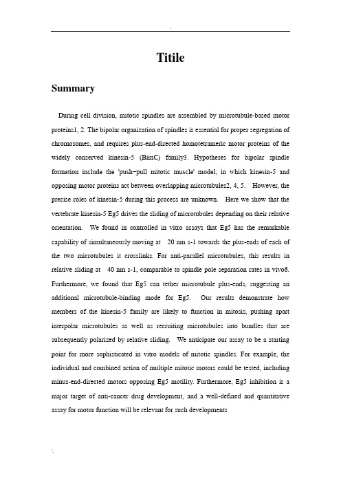
TitileSummaryDuring cell division, mitotic spindles are assembled by microtubule-based motor proteins1, 2. The bipolar organization of spindles is essential for proper segregation of chromosomes, and requires plus-end-directed homotetrameric motor proteins of the widely conserved kinesin-5 (BimC) family3. Hypotheses for bipolar spindle formation include the 'push−pull mitotic muscle' model, in which kinesin-5 and opposing motor proteins act between overlapping microtubules2, 4, 5. However, the precise roles of kinesin-5 during this process are unknown. Here we show that the vertebrate kinesin-5 Eg5 drives the sliding of microtubules depending on their relative orientation. We found in controlled in vitro assays that Eg5 has the remarkable capability of simultaneously moving at 20 nm s-1 towards the plus-ends of each of the two microtubules it crosslinks. For anti-parallel microtubules, this results in relative sliding at 40 nm s-1, comparable to spindle pole separation rates in vivo6. Furthermore, we found that Eg5 can tether microtubule plus-ends, suggesting an additional microtubule-binding mode for Eg5. Our results demonstrate how members of the kinesin-5 family are likely to function in mitosis, pushing apart interpolar microtubules as well as recruiting microtubules into bundles that are subsequently polarized by relative sliding. We anticipate our assay to be a starting point for more sophisticated in vitro models of mitotic spindles. For example, the individual and combined action of multiple mitotic motors could be tested, including minus-end-directed motors opposing Eg5 motility. Furthermore, Eg5 inhibition is a major target of anti-cancer drug development, and a well-defined and quantitative assay for motor function will be relevant for such developmentsContentTitile (1)Summary (1)1Introduction (1)1.1Restatement of the Problem (1)1.2Background (1)1.1.1Common Solving Technique (1)1.1.2Previous Works (1)1.3Example (1)2Analysis of the Problem (1)2.1Outline of the Approach (1)2.2Basic Assumptions (2)2.3Definitions and Key Terms (2)3Calculating and Simplifying the Model (2)4The Model Results (3)5Validating the Model (3)6Strengths and Weaknesses (3)6.1Strengths (3)6.2Weaknesses (3)7Food for Thought (3)8Conclusion (3)References (4)Appendices (4)Appendix A Source Code (4)Appendix B (4)1Introduction1.1Restatement of the Problem …1.2Background…1.1.1Common Solving Technique…1.1.2Previous Works…1.3Example…2Analysis of the Problem …2.1Outline of the Approach…2.2Basic Assumptions●●●●●2.3Definitions and Key Terms●●●●Table 1.…Symbol Meaning Unit3Calculating and Simplifying the Model …4The Model Results……5Validating the Model…6Strengths and Weaknesses6.1S trengths●●●●6.2W eaknesses●●●●7Food for Thought…8Conclusion….References…AppendicesAppendix A Source CodeHere are the simulation programmes we used in our model as follow. Input matlab source:……….Appendix B…….Input C++ source:…………..…………..。
- 1、下载文档前请自行甄别文档内容的完整性,平台不提供额外的编辑、内容补充、找答案等附加服务。
- 2、"仅部分预览"的文档,不可在线预览部分如存在完整性等问题,可反馈申请退款(可完整预览的文档不适用该条件!)。
- 3、如文档侵犯您的权益,请联系客服反馈,我们会尽快为您处理(人工客服工作时间:9:00-18:30)。
For office use only T1 ________________ T2 ________________ T3 ________________ T4 ________________ Team Control Number11111Problem ChosenABCDFor office use onlyF1 ________________F2 ________________F3 ________________F4 ________________ 2015Mathematical Contest in Modeling (MCM/ICM) Summary Sheet In order to evaluate the performance of a coach, we describe metrics in five aspects:historical record, game gold content, playoff performance, honors and contribution to the sports. Moreover, each aspect is subdivided into several secondary metrics. Take playoff performance as example, we collect postseason result (Sweet Sixteen, Final Four, etc.) per year from NCAA official website, Wikimedia and so on.First, ****grade.To eval*** , in turn, are John Wooden, Mike Krzyzewski, Adolph Rupp, Dean Smith and Bob Knight.Time line horizon does make a difference. According to turning points in NCAA history, we divide the previous century into six periods with different time weights which lead to the change of ranking.We conduct sensitivity analysis on FSE to find best membership function and calculation rule. Sensitivity analysis on aggregation weight is also performed. It proves AM performs better than single model. As a creative use, top 3 presidents(U.S.) are picked out: Abraham Lincoln, George Washington, Franklin D. Roosevelt.At last, the strength and weakness of our mode are discussed, non-technical explanation is presented and the future work is pointed as well.Key words: Ebola virus disease; Epidemiology; West Africa; ******ContentsI. Introduction (2)1.1 (2)1.2 (2)1.3 (2)1.4 (2)1.5 (2)1.6 (2)II. The Description of the Problem (2)2.1 How do we approximate the whole course of paying toll? (2)2.2 How do we define the optimal configuration? (2)2.3 The local optimization and the overall optimization (3)2.4 The differences in weights and sizes of vehicles (3)2.5 What if there is no data available? (3)III. Models (3)3.1 Basic Model (3)3.1.1 Terms, Definitions and Symbols (3)3.1.2 Assumptions (3)3.1.3 The Foundation of Model (4)3.1.4 Solution and Result (4)3.1.5 Analysis of the Result (4)3.1.6 Strength and Weakness (4)3.2 Improved Model (4)3.2.1 Extra Symbols (5)3.2.2 Additional Assumptions (5)3.2.3 The Foundation of Model (5)3.2.4 Solution and Result (5)3.2.5 Analysis of the Result (6)3.2.6 Strength and Weakness (6)IV. Conclusions (6)4.1 Conclusions of the problem (6)4.2 Methods used in our models (6)4.3 Applications of our models (6)V. Future Work (6)5.1 Another model (6)5.1.1 The limitations of queuing theory (6)5.1.2 (7)5.1.3 (7)5.1.4 (7)5.2 Another layout of toll plaza (7)5.3 The newly- adopted charging methods (7)VI. References (8)VII. Appendix (8)I. IntroductionIn order to indicate the origin of the toll way problems, the following background is worth mentioning.1.11.21.31.41.51.6II. The Description of the Problem2.1 How do we approximate the whole course of paying toll?●●●●2.2 How do we define the optimal configuration?1) From the perspective of motorist:2) From the perspective of the toll plaza:3) Compromise:2.3 The local optimization and the overall optimization●●●Virtually:2.4 The differences in weights and sizes of vehicles2.5 What if there is no data available?III. Models3.1 Basic Model3.1.1 Terms, Definitions and SymbolsThe signs and definitions are mostly generated from queuing theory.●●●●●3.1.2 Assumptions●●●●●3.1.3 The Foundation of Model1) The utility function●The cost of toll plaza:●The loss of motorist:●The weight of each aspect:●Compromise:2) The integer programmingAccording to queuing theory, we can calculate the statistical properties as follows.3)The overall optimization and the local optimization●The overall optimization:●The local optimization:●The optimal number of tollbooths:3.1.4 Solution and Result1) The solution of the integer programming:2) Results:3.1.5 Analysis of the Result●Local optimization and overall optimization:●Sensitivity: The result is quite sensitive to the change of the threeparameters●Trend:●Comparison:3.1.6 Strength and Weakness●Strength: In despite of this, the model has proved that . Moreover,we have drawn some useful conclusions about . The model is fit for,such as●Weakness: This model just applies to . As we have stated, . That’sjust what we should do in the improved model.3.2 Improved Model3.2.1 Extra SymbolsSigns and definitions indicated above are still valid. Here are some extra signs and definitions.●●●●3.2.2 Additional Assumptions●●●Assumptions concerning the anterior process are the same as the Basic Model.3.2.3 The Foundation of Model1) How do we determine the optimal number?As we have concluded from the Basic Model,3.2.4 Solution and Result1) Simulation algorithmBased on the analysis above, we design our simulation arithmetic as follows.●Step1:●Step2:●Step3:●Step4:●Step5:●Step6:●Step7:●Step8:●Step9:2) Flow chartThe figure below is the flow chart of the simulation.3) Solution3.2.5 Analysis of the Result3.2.6 Strength and Weakness●Strength: The Improved Model aims to make up for the neglect of .The result seems to declare that this model is more reasonable than the Basic Model and much more effective than the existing design.●Weakness: . Thus the model is still an approximate on a large scale.This has doomed to limit the applications of it.IV. Conclusions4.1 Conclusions of the problem●●●4.2 Methods used in our models●●●4.3 Applications of our models●●●V. Future Work5.1 Another model5.1.1 The limitations of queuing theory5.1.25.1.35.1.41)●●●●2)●●●3)●●●4)5.2 Another layout of toll plaza5.3 The newly- adopted charging methodsVI. References[1][2][3][4]VII. Appendix欢迎您的下载,资料仅供参考!致力为企业和个人提供合同协议,策划案计划书,学习资料等等打造全网一站式需求。