第1课 FDTD基础
matlab实现一维fdtd仿真

麦克斯韦方程组为
(2—1—1)
(2—1—2)
各项同性线性介质中的本构关系为
(2—1—3)
在直角坐标系中,(2—1—1)、(2—1—2)式写为
(2—1—4)
以及
(2—1—5)下面我们考虑(2—1—4)、(2—1—5)式的FDTD差分离散。令 代表 或 直角坐标系中某一分量,在时间和空间域中的离散取以下符号表示:
FDTD在电磁研究的多个领域获得广泛应用,其中有:辐射天线的分析,微波器件和导行波结构的研究,散射和雷达截面计算,周期机构分析,电子封装和电磁兼容分析,核电磁脉冲的传播和散射,微光学元器件中光的传播和颜射特性。
二、FDTD模拟电磁波传播的原理
麦克斯韦方程组是支配宏观电磁现象的一组基本方程。这组方程既可以写成微分形式,又可以写成积分形式。FDTD方法是由微分形式的麦克斯韦旋度方程出发进行差分离散从而得到一组时域推进公式。首先给出麦克斯韦旋度方程及其在直角坐标系中的FDTD离散形式,由三维情况到一维情况,即一维电磁波传播的理论基础。
c = 1/sqrt(mu_0*eps_0); %光速
%定义问题空间和参数
domain_size = 1; %空间问题的长度
dx = 1e-3; %单元网格大小
dt = 3e-12; %步长时间的持续
number_of_time_steps = 2000; %迭代次数
nx = round(domain_size/dx); %在问题空间的单元数目
3.2参数设置
程序设计了电流屏在z轴上传播,产生的电场和磁场,此电流屏放置在问题空间的中心,与两个相互平行的完善导体平面平行,整个区间充满空气。激励源在两板之间传播和反射。
无论是简单目标还是复杂目标,在进行FDTD离散时网格尺寸的确定,除了受计算资源的限制不可能取得很小外,还需要考虑以下几个因素:
第1课 FDTD基础
近似:
f n ( x, y, z) x
x ix
f n (i 1 , j, k ) f n (i 1 , j
f n (i, j 1 , k ) 2
f
n (i,
j
1 2
,k)
y y jy
y
f n ( x, y, z) z
z k z
f n (i, j, k 1 ) f n (i, 2 z
K.S. Yee. Numerical solution of initial boundary value problems involving Maxwell's equations in isotropic media. IEEE Trans. Antennas Propagat. 14: 302‐307, 1966
Nanjing University of Science & Technology
计算电磁学
Unit 1: 时域有限差分方法
樊振宏
研究背景
近年来,微波和毫米波通信、航空航天、雷达、精确制导等 民用军用系统朝着高频化、微型化、多功能、高可靠性以及低 成本方向发展。 由于色散、不连续性和封装而产生的失真与 时延,以及由于耦合而产生的串音噪声等问题变得十分严重, 传统的准静设计方法已不能满足设计要求,必须采用精确的电 磁场全波分析方法。
14
Ey
Ex
Hz
(i,j,k+1) Ez Hx
Hy
(i,j+1,k)
(i+1,j,k)
z y
(i+1,j+1,k) x
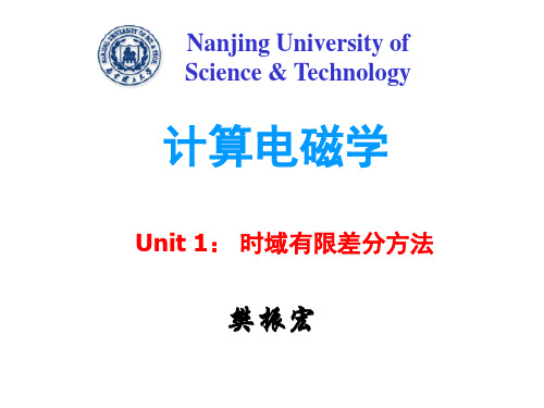
场分量的空间编号,采用上面的场量空间离散定义,定义各方向上
Ex
E x t
[文库精品]fod培训课件
![[文库精品]fod培训课件](https://img.taocdn.com/s3/m/11f24e670622192e453610661ed9ad51f11d5474.png)
3
发展趋势
未来fod将朝着小型化、集成化、智能化方向发 展。
fod的用途与价值
用途
fod被广泛应用于光纤通信网络、CATV网络、数据中心、云 计算等领域,作为光信号的分发和接收端口。
价值
fod能够实现光信号的高效分路和传输,提高网络系统的可靠 性和稳定性,降低传输成本,具有重要的应用价值。
02
fod培训内容
fod的基本概念与原理
总结词
理解fod的背景和意义
详细描述
介绍fod的起源、发展历程和在当今社会中的应用价值,阐述其基本概念和原 理,包括fod的定义、特点和优势等。
Байду номын сангаас
fod的操作方法与技巧
总结词
掌握fod的实践技能
详细描述
详细讲解fod的操作方法和技巧,包括如何进行fod的准备工作、操作流程、注意 事项等,同时提供相关案例和实际操作演示,帮助学员更好地掌握fod的实践技 能。
建议
在参加fod培训时,学员应该注重理论与实践相结合,多进行 实践操作,加深对理论知识的理解。同时,学员应该注重创 新思维能力的培养,提出自己的见解和思路,为fod技术的发 展做出贡献。
THANKS
谢谢您的观看
提高实践操作能力
通过大量的实践操作,使学员能够熟练掌握fod技术的实 际应用技能。
培养创新思维能力
鼓励学员在学习过程中提出自己的见解和思路,培养创 新思维能力。
对参加fod培训的期望与建议
期望
参加fod培训的学员应该具备基本的计算机操作能力和英语阅 读能力,能够独立完成实验和作业。同时,学员应该认真学 习,积极参与讨论和交流,提高自己的学习效果。
类型
根据不同的应用场景和需求, fod有不同的类型,如室内型、 室外型、盒式、带保护套筒等
FDTD

3. The Finite-Difference Time-
Domain Method (FDTD)
The Finite-Difference Time-Domain method (FDTD) is today’s one of the most popular technique for the solution of electromagnetic problems. It has been successfully applied to an extremely wide variety of problems, such as scattering from metal objects and dielectrics, antennas, microstrip circuits, and electromagnetic absorption in the human body exposed to radiation. The main reason of the success of the FDTD method resides in the fact that the method itself is extremely simple, even for programming a three-dimensional code. The technique was first proposed by K. Yee, and then improved by others in the early 70s.
TOFD普及班培训教材

3.4.2 信号的位置测量 ................................................................................. 33
3.5 TOFD 技术的盲区和扫查误差....................................................................... 34
FDTD入门教程

欢迎进入FDTD Solutions 的入门教程!入门教程由四章内容组成。
第一章介绍FDTD Solutions 的基本功能,以及器件建构,程序运行和结果分析。
后面三章则针对v个实际问题,提供详细指导,帮助用户一步步地了解每一模块的功能及其使用。
文中涉及的所有模拟设计文件都可以从LUMERICAL 的相应网页上免费下载。
第一章简介第二章银质纳米线谐振腔散射教程第三章环形谐振腔教程第四章光子晶体微腔教程简介The goal of the Getting Started Guide is to introduce the Finite Difference Time Domain (FDTD) technique and explain how modeling is done with the software.The FDTD algorithm is useful for design and investigation in a wide variety of applications involving the propagation of electromagnetic radiation through complicated media. It is especially useful for describing radiation incident upon or propagating through structures with strong scattering or diffractive properties. The available alternative computational methods - often relying on approximate models - frequently provide inaccurate results. FDTD Solutions is useful for numerous engineering problems of commercial interest including:• display technologies• optical storage devices• LED design• biophotonic sensors• plasmon polariton resonance devices• optical waveguide devices• photonic crystal devices• integrated optical filters• optical micro cavity designFDTD Solutions is an accurate and easy to use, versatile design tool capable of treating this wide variety of applications. This introductory chapter of the Getting Started Guide introduces the general FDTD method and provides a basic overview of the product usage. The final sections contain examples that are accompanied by step-by-step instructions so that you can set up and run the simulations yourself.什么是时域有限差分?The Finite Difference Time Domain (FDTD) method has become the state-of-the-art method for solving Maxwell’s equations in complex geometries. It is a fully vectorialmethod that naturally gives both time domain , and frequency domain information to the user, offering unique insight into all types of problems and applications inelectromagnetics and photonics .The technique is discrete in both space and time . The electromagnetic fields and structural materials of interest are described on a discrete mesh made up of so-called Yee cells . Maxwell’s equations are solved discretely in time, where the time step used is related to the mesh size through the speed of light. This technique is an exactrepresentation of Maxwell’s equations in the limit that the mesh cell size goes to zero. Structures to be simulated can have a wide variety of electromagnetic material properties. Light sources may be added to the simulation. The FDTD method is used to calculate how the EM fields propagate from the source through the structure . Subsequent iteration results in the electromagnetic field propagation in time. Typically, the simulation is run until there are essentially no electromagnetic fields left in the simulation region.Time domain information can be recorded at any spatial point (or group of points). This data can be recorded for the duration of the simulation, or it can be recorded as a series of "snapshots" at times specified by the user.Frequency domain information at any spatial point (or group of points) may be obtained through the Fourier transform of the time domain information at that point. Thus, the frequency dependence of power flow and modal profiles may be obtained over a wide range of frequencies from a single simulation.In addition, results obtained in the near field using the FDTD technique may be transformed to the far field, in applications where scattering patterns are important.More information about the FDTD method, including references, can be found in the Physics of the FDTD Algorithm section of the reference guide.FDTD的用户界面This section discusses useful features of the FDTD Solutions Graphical User Interface (GUI).In this topicGraphical User Interface: Windows andToolbarsAdd Objects to the simulationEdit ObjectsStart a new 2D/3D simulationGraphical User Interface: Windows and ToolbarsThe graphical user interface contains useful tools for editing simulations, including• a toolbar for adding objects to the simulation• a toolbar to edit objects• a toolbar to run simulations•an objects tree to show the objects which are currently included in the simulation• a script file editor window•an object library• a window to set up parameter sweeps and optimizationsIn the default configuration some of the Windows are hidden. To open hidden windows, click the right mouse button anywhere on the main title bar or the toolbar to get the pop up window shown in the screen shot below. The visible windows/toolbars have a check mark next to their name; the hidden ones do not have check marks. A second way to obtain the pop up window is to go to the main title toolbar and select VIEW->WINDOWS.For more information about the toolbars and windows see the Layout editor section of the reference guide.Add Objects to the simulationThe Graphical User interface contains buttons to add objects to the simulation. Click on the arrow next to the image to get a pull down menu which shows all the available options in a group. The screenshot below shows what happens when we click on the arrow next to the COMPONENTS button. Note that the picture on the button is the same as the MORE CHOICES option in the list. If we click on the button itself (instead of the arrow) we will go directly to the MORE CHOICES section of the object library.Also notice that the picture for the COMPONENTS button will change depending on what the last component that was added to the simulation was. Finally, the ZOOM EXTENTbutton in the toolbar will resize the viewports to fit all the objects currently included in the simulation.Edit objectsTo edit an object, select the object and press E on the keyboard or press the EDIT buttonon the toolbar. The easiest way to select an object is to click on the name of the object in the objects tree. However, objects can also be selected by clicking on the graphical depiction of them when the SELECT button is pressed. For more information see the Layout editor section of the reference guide.When we edit objects in FDTD, we get an edit window. The edit windows have units for the settings; in the GEOMETRY tab, the x, y and z location will be in μm by default. The units can be changed to nm if we choose SETTINGS->LENGTH units in the main menu. Fields in the edit windows act like calculators, so that equations can be entered in the fields. See the y span field below for an example.Start a new 2D/3D simulationBy default FDTD Solutions opens with a blank 3D simulation. In the following Getting Started Examples, we often begin with a 2D simulation, which can be obtained as shown in the screenshot below.模拟运行与优化This section discusses important checks which should be made before running a simulation (memory requirements, material fits) and gives links to more information about running simulations and parameter sweeps or optimizations.In this topicCheck memory requirementsCheck material fitsSetup parallel optionsRun simulationRun parameter sweeps and optimizationsCheck memory requirementsTo check the memory requirements, press the CHECK button If this is not the current icon, you can find it by pressing the arrow. Note that the memory report indicates the amount of memory used by each object in the simulation project as well as the total memory requirements. This allows for judicious choice of monitor properties in large and extensive simulations.Check material fitsThe CHECK button also contains a material explorer option . Many of the materials used in FDTD Simulations come from experimental data (see the materials section of the Reference Guide for references for the material data and descriptions of the FDTD material models). Before running a simulation, FDTD Solutions automatically generates a multi-coefficient model fit to the material data in the wavelength range for the source. It is a good idea to check and optimize the material fit before running a simulation. Setup the resource configurationBefore running any simulations, the resource options must be set up. These options canbe accessed by pressing the Resources button . In most cases, the default settings should be fine. The 'number of processes' is typically set to the number of cores in your computer.Run simulationYou can run simulations by pressing the RUN button on the mail toolbar. For more details, such as how to run multiple simulations in distributed mode, please see the RunSimulations section in the online User Guide, or the Running simulations and analysis section of the Reference Guide.Run parameter sweeps and OptimizationsFDTD Solutions also has a built in parameter sweep and optimization window. This window can be seen at the top of the page, and can be opened using the instructions in the Graphical User Interface discussion just prior to this topic.Optimization Window includes buttons to add a parameter sweep and add an optimization. Parameter sweeps and optimizations can include multiple parameters, or be nested. Each optimization or sweep can be run by pressing the right-most button.仿真数据分析This section discusses the tools used to analyze simulation data: the Analysis Window, the script environment and data export to third party software such as MATLAB. For more details please see the Analysis tools and the Scripting language chapters in the Reference Guide.In this topicAnalysis windowScriptingData exportAnalysis windowThe screen shot below shows the open analysis window. The analysis window can be used to plot monitor data.A variety of monitor data can be plotted via the Analysis window, depending on the monitor type. Spatial refractive index data, field vs time, field vs frequency, fields vs spatial dimensions, and power transmission vs frequency are a few examples. The terminology 'Intensity' indicates a squared quantity. For example, 'E intensity' means |E|^2. 'Ex intensity' means |Ex|^2. Field data from frequency monitors is always plotted as an Intensity. If you want to see the real or imaginary parts of the field, or if you want to obtain phase information, the scripting language will be required.ScriptingFDTD Solutions contains a built in scripting language which can be used to obtain simulation data, and do plotting or post-processing of data. The script prompt can be used to execute a few commands, or the built in script file editor can be used to create more complex scripts.A thorough introduction to the Lumerical scripting language can be found in the Scripting section of the FDTD Solutions online user guide. Definitions for all of the script commands are given in the Scripting language chapter in the Reference Guide.Data ExportFDTD simulation data can be exported into text file format using the analysis window, into a Lumerical data file format (*.ldf) which can be loaded into another simulation, or into a Matlab data (*.mat) file. Instructions for exporting to these file formats can be found in the links under the Scripting section.银质纳米线谐振腔散射教程问题综述当光波入射到金属纳米粒子上时,光与金属表面附近的电荷密度相互作用产生的表面等离子体极化surface plasmon polaritons 扮演着重要角色。
fdtd基本原理
1 1 nz 2 1 1 1 nz 2 n z 1 nz H y (t ) [ E x (t ) E x (t )] J my (t ) t 0 z 0
1 1 1 t t H y ( z, t ) [H y (nz ) H y (nz )] O[(z)2 ] z z 2 2 z n z z
( 19)
由(14)与(18)可得(8b)的差分形式:
FDTD基本原理
H
1 1 ( n z , nt ) 2 2 y
H t
1 1 ( n z , nt ) 2 2 y
1 1 1 1 nz 2 n z 1 nz [ E x (t ) E x (t )] J my (t ) 0 z 0
( nz 1/ 2, nt 1/ 2) Hy
( n z 2 , nt ) Ex
( n z 1, nt ) Ex
E x( n z , nt )
z 2
nz 1 / 2
E x( n z 1, nt )
z 2
nz 1 / 2
z 2
nz 2
z 2
nz 3 / 2 nz 1
ห้องสมุดไป่ตู้
1
1
( 21)
由(20)整理可得:
H
1 1 ( n z , nt ) 2 2 y
H
1 1 ( n z , nt ) 2 2 y
t t ( n z 2 , n t ) ( n z 1, n t ) ( n z , nt ) [E Ex ] J 0 z x 0 my
H
y
(nz 3/ 2)
(nz 1/ 2)
(nz 1/ 2)
FDTD原理及例子ppt课件
H D J t
E B t
•B 0
•D
时谐场形式:
H
D t
Je, Je
E
B E t Jm , Jm sH
• B m
• D e
H j( j )E
E jH
E(x, y, z, t) E0 (x, y, z,t)e jt H (x, y, z, t) H0 (x, y, z,t)e jt
)
z r (k)
只要给定了所有空间点上电/磁场的初值,就可以一步一步地求出任 意时刻所有空间点上的电/磁场值。
一维Maxwell方程的Yee算法
Ex Hy
Ex
n2 n 3/2
Hy Ex
n 1 n 1/ 2
n0
0
1
2
3k
H~
n1/ 2 y
(k
1) 2
H~
n1/ 2 y
(k
1) 2
ct zr (k
FDTD数值分析法
目录
1.麦克斯韦方程的基础知识 2.一维和三维Maxwell方程的Yee算法 3.数值稳定性分析 4.吸收边界条件 5.波源的设置 6.编程思路
麦克斯韦方程微分形式:
BPM 方式
基础知识
H D J t
E B t
•B 0
•D
基础知识
麦克斯韦方程微分形式:
FDTD方式将时间进 行差分,并且磁场与 电场交替迭代更新
DbHy i,
j,
k
Ex i,
j,
k
x
1, n
z
Ex i,
j, k, n
H z i, j, k, n 1 DaHz i, j, kH z i, j, k, n
FDTD基础
Mathematic Basis
Forward Difference
f ( x0 x) f ( x0 ) f ' ( x0 ) x
f ( x)
Backward Difference
f ' ( x0 )
f ( x0 ) f ( x0 x) x
x 0 x
K.S. Yee. Numerical solution of initial boundary value problems involving Maxwell's equations in isotropic media. IEEE Trans. Antennas Propagat. 14: 302‐307, 1966
J E Jm mH
D E B H
4
FDTD简介
时域有限差分法 ( Finite‐Difference Time‐Domain, FDTD) 是对时域 Maxwell方程进行差分离散的方式,是 电磁场计算领域的一种常用方法。FDTD 由 K. S. Yee 在 1966 年在其论文中提出,其模型基础就是电动力学中最基 本的麦克斯韦方程( Maxwell's equation ) 。在 FDTD 方法提出之后,随着计算技术,特别是电子计算机技术的发 展,FDTD 方法得到了长足的发展,在电磁学,电子学,光 学等领域都得到了广泛的应用。
5
葛德彪,闫玉波. 电磁波时域有限差分方法(研究生教学用书) . 西安电子科技大 学出版社, 版本: 第2版, 西安电子科技大学出版社. 2005
王秉中.计算电磁学.科学出版社.2005
盛新庆. 计算电磁学要论(第2版).中国科学技术大学出版社2008
计算电磁学之FDTD算法的MATLAB语言实现
South China Normal University课程设计实验报告课程名称:计算电磁学指导老师:专业班级: 2014级电路与系统姓名:学号:FDTD算法的MATLAB语言实现摘要:时域有限差分(FDTD)算法是K.S.Yee于1966年提出的直接对麦克斯韦方程作差分处理,用来解决电磁脉冲在电磁介质中传播和反射问题的算法。
其基本思想是:FDTD计算域空间节点采用Yee元胞的方法,同时电场和磁场节点空间与时间上都采用交错抽样;把整个计算域划分成包括散射体的总场区以及只有反射波的散射场区,这两个区域是以连接边界相连接,最外边是采用特殊的吸收边界,同时在这两个边界之间有个输出边界,用于近、远场转换;在连接边界上采用连接边界条件加入入射波,从而使得入射波限制在总场区域;在吸收边界上采用吸收边界条件,尽量消除反射波在吸收边界上的非物理性反射波。
本文主要结合FDTD算法边界条件特点,在特定的参数设置下,用MATLAB语言进行编程,在二维自由空间TEz网格中,实现脉冲平面波。
关键词:FDTD;MATLAB;算法1 绪论1.1 课程设计背景与意义20世纪60年代以来,随着计算机技术的发展,一些电磁场的数值计算方法逐步发展起来,并得到广泛应用,其中主要有:属于频域技术的有限元法(FEM)、矩量法(MM)和单矩法等;属于时域技术方面的时域有限差分法(FDTD)、传输线矩阵法(TLM)和时域积分方程法等。
其中FDTD是一种已经获得广泛应用并且有很大发展前景的时域数值计算方法。
时域有限差分(FDTD)方法于1966年由K.S.Y ee提出并迅速发展,且获得广泛应用。
K.S.Y ee用后来被称作Y ee氏网格的空间离散方式,把含时间变量的Maxwell旋度方程转化为差分方程,并成功地模拟了电磁脉冲与理想导体作用的时域响应。
但是由于当时理论的不成熟和计算机软硬件条件的限制,该方法并未得到相应的发展。
20世纪80年代中期以后,随着上述两个条件限制的逐步解除,FDTD便凭借其特有的优势得以迅速发展。
- 1、下载文档前请自行甄别文档内容的完整性,平台不提供额外的编辑、内容补充、找答案等附加服务。
- 2、"仅部分预览"的文档,不可在线预览部分如存在完整性等问题,可反馈申请退款(可完整预览的文档不适用该条件!)。
- 3、如文档侵犯您的权益,请联系客服反馈,我们会尽快为您处理(人工客服工作时间:9:00-18:30)。
0
H x t
n
1 2
1 n 1 1 1 1 2 i, j , k H x i, j , k 2 2 2 2
21
E update equations
1 1 t Exn 1 (i , j, k ) Exn (i , j , k ) 2 2 1 1 1 n n n n 1 1 1 1 1 1 1 1 1 2 2 2 2 H z (i , j , k ) H z (i , j , k ) H y (i , j , k ) H y (i , j, k ) 2 2 2 2 2 2 2 2 y z 1 1 t E yn 1 (i, j , k ) E yn (i, j , k ) 2 2 1 1 1 n n n n 1 1 1 1 1 1 1 1 1 2 2 2 2 H ( i , j , k ) H ( i , j , k ) H ( i , j , k ) H ( i , j , k) x x z z 2 2 2 2 2 2 2 2 z x 1 1 t Ezn 1 (i, j, k ) Ezn (i, j , k ) 2 2 1 1 1 n n n n 1 1 1 1 1 1 1 1 1 2 2 2 2 H ( i , j , k ) H ( i , j , k ) H ( i , j , k ) H ( i , j , k ) y y x x 2 2 2 2 2 2 2 2 x y
Yee网格的特点
Yee网格体系的特点是,E和H各分量在空间的取值点被交叉 放置,使得在每个坐标平面上每个E分量由四个H分量环绕, 同时每个H分量由四个E分量环绕。这样的电磁场空间分布符 合电磁场的基本规律――法拉第电磁感应定律和安培环路定 律的自然结构,即符合麦克斯韦方程的基本要求,能够恰当 地描述电磁场的传播特性。 为实现空间坐标的差分计算,并考虑导电磁场在空间相互正 交和交链的关系,在Yee网格中,每个坐标轴方向上场分量 间相距半个网格空间步长,因而同一种场分量之间相隔一个 空间步长:电场和磁场在时间顺序上相隔半个时间步长,这 样,使麦克斯韦方程离散后可以构成显式差分方程,从而给 出电磁问题的初始值后,可以在时间上迭代求解。
Nanjing University of Science & Technology
计算电磁学
Unit 1: 时域有限差分方法
樊振宏
研究背景
近年来,微波和毫米波通信、航空航天、雷达、精确制导等 民用军用系统朝着高频化、微型化、多功能、高可靠性以及低 成本方向发展。 由于色散、不连续性和封装而产生的失真与 时延,以及由于耦合而产生的串音噪声等问题变得十分严重, 传统的准静设计方法已不能满足设计要求,必须采用精确的电 磁场全波分析方法。
x E z H
y E
(i,j,k +1 )
z k) z ( i+1 ,j,k) ( i+1 ,j +1 ,k) x
y
1 n 1 1 n E i , j , k 1 E i , j , k y y z 2 2
1 1 n 1 n E i , j , k E i , j , k x x t 2 2
20
H公式推导举例
H x Ez E y 0 y z t
1 n 1 1 n E z i, j 1, k E z i, j , k y 2 2
(Ampere’s law)
(Faraday’s law) 各向同性介质中的本构关系为:
D E B H
5
FDTD简介
时域有限差分法 ( Finite‐Difference Time‐Domain, FDTD) 是对时域 Maxwell方程进行差分离散的方式,是 电磁场计算领域的一种常用方法。FDTD 由 K. S. Yee 在 1966 年在其论文中提出,其模型基础就是电动力学中最基 本的麦克斯韦方程( Maxwell's equation ) 。在 FDTD 方法提出之后,随着计算技术,特别是电子计算机技术的发 展,FDTD 方法得到了长足的发展,在电磁学,电子学,光 学等领域都得到了广泛的应用。
E y
E z H x mH x z y t
H y Ez E x mH y x z t
E y H x H z E y z x t
H y
H x E z E z x y t
E x E y H z mHz y x t
电磁分析的本质是求解Maxwell Equation 在特定初始条件特 定边界条件下 边界的复杂,导致传统的解析分析方法无法胜任
2
计算电磁学的应用领域
3
电磁场全波分析方法分类
基于微分方程模型的分析方法 时域有限差分 频域有限差分 有限元 FDTD – Finite Difference Time Domain FDFD – Finite Difference Frequency Domain FEM – Finite Element Method
11
FDTD
FDTD法对电磁场E、H分量在空间和时间上采取交替抽样的
离散方式,每一个E(或H )场分量周围有四个H(或E )
场分量环绕,应用这种离散方式将含时间变量的麦克斯韦 旋度方程转化为一组差分方程,用具有相同电参量的空间
网格去模拟被研究对象,选取适当的场初始值和计算空间
的边界条件,在时间轴上逐步推进地求解空间电磁场。
各向同性介质中的本构关系为:
D E B H
18
直角坐标系中的FDTD方程
六个标量场方程
E x H z H y E x y z t
E y
E z H x mH x z y t
H y Ez E x mH y x z t
14
Ey Ex (i,j,k +1) Ez Hx Hz
Hy
(i,j+1,k) z (i+1 ,j,k) y (i+1,j+1,k) x
场分量的空间编号,采用上面的场量空间离散定义,定义各方向上 的 Yee 元胞棱边为整数n编号,棱边的中间位置为半整数 n+1/2 的自然编号。以 Yee 元胞的角点为整数网格点为参考点编号,如 图中的各坐标方向最小的左下点为整数的(i, j, k)离散点,相对于参 考编号点,相差多少网格,即相差几个编号,对于相差半个网格的 场量位置,用 1/2 表示半个网格。如Ex 分量,在 x 方向位于半个 网格上,用 1/2 表示,而在 y、z 方向上位于整数网格上,用整数 表示,即 Ex (i +1/2, j, k) ,其他电场分量也是类似编号;对于 Hx 分量,在 x方向位于整网格线上,而在 y、z 方向上,位于半个 网格上,即 Hx (i, j +1/2, k +1/2) ,其他磁场分量也是类似编 15 号。
基于积分方程模型的分析方法 矩量法 MoM – Method of Moment
基于矩量法的快速算法
4
3-D Maxwell’s Equations
H D / t J E B / t J m
J E Jm mH
(i+1 ,j,k)
x
在 Yee 元胞结构上,6 个场分量在 Yee 元胞的表面上进行离散,在空间上, 各电场分量Ex Ey Ez在 Yee 元胞的棱边中间离散;各磁场分量 Hx Hy Hz 在 Yee 元胞表面的中间离散。在时间上,各电场分量分布在元胞棱边上, 方向与棱边一致,属于整数网格线上,这样电场分量在整时刻离散;各磁场 分量分布在元胞面的中间,其方向垂直元胞面,指向半网格位置,这样磁场 分量在半时刻离散。
K.S. Yee. Numerical solution of initial boundary value problems involving Maxwell's equations in isotropic media. IEEE Trans. Antennas Propagat. 14: 302‐307, 1966
16
Hx对应Yee元胞表面上各场量分布示意
17
3-D Maxwell’s equations
H D / t J E B / t J m
J E Jm mH
(Ampere’s law)
(Faraday’s law)
6
葛德彪,闫玉波. 电磁波时域有限差分方法(研究生教学用书) . 西安电子科技大 学出版社, 版本: 第2版, 西安电子科技大学出版社. 2005
王秉中.计算电磁学.科学出版社.2005
盛新庆. 计算电磁学要论(第2版).中国科学技术大学出版社2008
7
旋度方程展开为六个标量场方程
E x H z H y E x y z t
8
Mathematic Basis
Forward Difference
f ( x0 x) f ( x0 ) f ' ( x0 ) x
f ( x)
Backward Difference
f ' ( x0 )
f ( x0 ) f ( x0 x) x
x0 x
Central Difference
x E z H
y E
(i,j,k +1 )
z E y H