MIT公开课:单变量微积分讲义unit1(1~7)
单变量微积分笔记7
单变量微积分笔记7曲线构图的目标是根据f’(x)和f’’ (x)画出原函数f(x)的图像。
原函数:f(x) = 3x-x3f’(x) = 3-3x2f’’(x) = -6x函数的凹凸性前提是:设f(x)在[a,b]上连续,在(a,b)内具有一阶和二阶导数。
如果函数f’(x) > 0,则f(x)在(a,b)内是递增的;如果f’(x) < 0,则f(x)在(a,b)内是递减的。
这很好理解,f’(x)是f(x)在x点切线的斜率,只有函数递增时,切线的斜率才能大于0。
如果f’’(x) > 0,则f’递增;如果f’’(x) < 0,则f’递减。
这相当于上一条结论的扩展,因为f’’是f’的导函数。
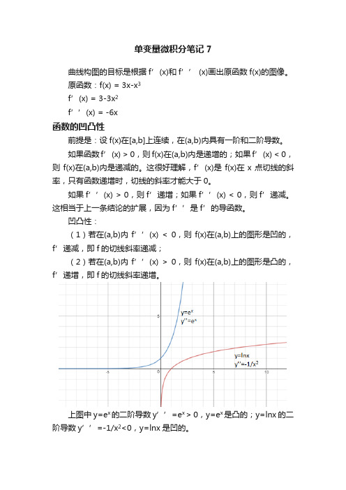
凹凸性:(1)若在(a,b)内f’’(x) < 0,则f(x)在(a,b)上的图形是凹的,f’递减,即f的切线斜率递减;(2)若在(a,b)内f’’(x) > 0,则f(x)在(a,b)上的图形是凸的,f’递增,即f的切线斜率递增。
上图中y=e x的二阶导数y’’=e x > 0,y=e x是凸的;y=lnx的二阶导数y’’=-1/x2<0,y=lnx是凹的。
奇怪的是,国内外的教材对凸凹的定义是不一样的。
同济大学的教材中,f’’大于0,函数为凹,f’’小于0,函数为凸,跟上面的定义正好相反。
在一些微积分教材中,有将凸称为上凸,凹成为下凸;还有反着叫的……越来越乱了。
极值点和驻点原函数f(x) = 3x-x3f’(x) = 3 - 3x2 = 3(1-x2)由此可以画出f(x)的简图:(-1, -2)和(1, 2)是两个重要的点,经过这两个点后,f’的符号改变,f的递增递减发生变化,在这两个点上,f’(x)=0,这两个点称为函数的极值点。
需要注意的是,极值点不是最值点,仅仅决定了导数的符号改变。
当f’(x0) = 0时,称x0为驻点,f(x0)为驻点值。
原函数f(x)=3x-x3有±1两个驻点,对应的驻点值为±2。
MIT微分方程课程表
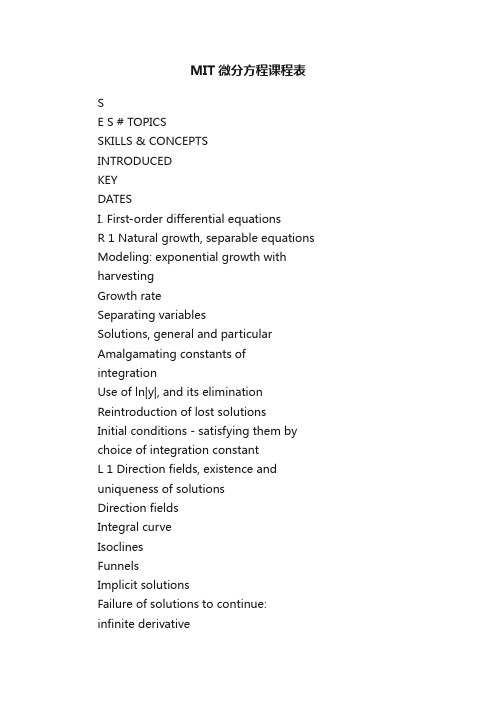
MIT微分方程课程表SE S # TOPICSSKILLS & CONCEPTS INTRODUCEDKEYDATESI. First-order differential equationsR 1 Natural growth, separable equations Modeling: exponential growth with harvestingGrowth rateSeparating variablesSolutions, general and particular Amalgamating constants of integrationUse of ln|y|, and its elimination Reintroduction of lost solutionsInitial conditions - satisfying them by choice of integration constantL 1 Direction fields, existence and uniqueness of solutionsDirection fieldsIntegral curveIsoclinesFunnelsImplicit solutionsFailure of solutions to continue: infinite derivativeR 2 Direction fields, integral curves, isoclines, separatrices, funnelsSeparatrixExtrema of solutionsL2Numerical methods Euler's methodL 3 Linear equations, modelsFirst order linear equationSystem/signal perspectiveBank account modelRC circuitSolution by separation if forcing termis constantR3Euler's method; linear models Mixing problems L 4 Solution of linear equations, integrating factorsHomogeneous equation, null signal Integrating factorsTransientsDiffusion example; coupling constantR 4 First order linear ODEs; integrating factorsSinusoidal input signalL 5 Complex numbers, roots of unity Complex numbersRoots of unityPS 2 outL Complex exponentials; sinusoidal Complex exponential 6 functions Sinusoidal functions: Amplitude,Circular frequency, Phase lagL 7 Linear system response to exponentialand sinusoidal input; gain, phase lagFirst order linear response toexponential or sinusoidal signalComplex-valued equation associatedto sinusoidal inputPS: half lifeR 5 Complex numbers; complex exponentialsL 8 Autonomous equations; the phase line,stabilityAutonomous equationPhase lineStabilitye^{k(t-t_0)} vs ce^{kt}PS 2 due;PS 3 outL9Linear vs. nonlinear Non-continuation of solutions R6Review for exam IExam IHour exam III. Second-order linear equationsR 7 Solutions to second order ODEsHarmonic oscillatorInitial conditionsSuperposition in homogeneous caseL1 1 Modes and the characteristic polynomial Spring/mass/dashpot systemGeneral second order linear equation Characteristic polynomialSolution in real root caseL 12 Good vibrations, damping conditions Complex rootsUnder, over, critical dampingComplex replacement, extraction ofreal solutionsTransienceRoot diagramR 8 Homogeneous 2nd order linear constant coefficient equationsGeneral sinusoidal responseNormalized solutionsL 13 Exponential response formula, spring driveDriven systemsSuperpositionExponential response formulaComplex replacementSinusoidal response to sinusoidalsignalR9Exponential and sinusoidal input signalsL Complex gain, dashpot drive Gain, phase lag PS 3 due;14 Complex gain PS 4 outL 15 Operators, undetermined coefficients,resonanceOperatorsResonanceUndetermined coefficientsR 10 Gain and phase lag; resonance; undetermined coefficientsL16Frequency response Frequency responseR11Frequency response First order frequency responseL 17 LTI systems, superposition, RLCcircuits.RLC circuitsTime invariancePS4 due;PS 5 outL18Engineering applications Damping ratio R12Review for exam IIL 19 Exam IIHourExam IIIII. Fourier seriesR13Fourier series: introduction Periodic functions L 20 Fourier seriesFourier seriesOrthogonalityFourier integralL 21 Operations on fourier series SquarewavePiecewise continuityTricks: trig id, linear combination,shiftR14Fourier series Different periodsL 22 Periodic solutions; resonance Differentiating and integrating fourier seriesHarmonic responseAmplitude and phase expression for Fourier seriesR15Fourier series: harmonic responseL 23 Step functions and delta functions Step functionDelta functionRegular and singularity functions Generalized functionGeneralized derivativePS 5 due;PS 6 outL 24 Step response, impulse responseUnit and step responsesRest initial conditionsFirst and second order unit step or unit impulse response R 16 Step and delta functions, and step and delta responses L 25 ConvolutionPost-initial conditions of unit impulseresponseTime invariance: Commutation withDTime invariance: Commutation witht-shiftConvolution productSolution with initial conditions as w *qR17Convolution Delta function as unit for convolutionL 26 Laplace transform: basic propertiesLaplace transformRegion of convergenceL[t^n]s-shift ruleL[sin(at)] and L(cos(at)]t-domain vs s-domainPS 6 due;PS 7 outL 27 Application to ODEsL[delta(t)]t-derivative ruleInverse transformPartial fractions; coverupNon-rest initial conditions for firstorder equationsR 18 Laplace transformUnit step response using Laplace transform.L 28 Second order equations; completing the squaress-derivative ruleSecond order equationsR19Laplace transform IIL 29 The pole diagramWeight and transfer functionL[weight function] = transfer functiont-shift rulePolesPole diagram of L T and long term behaviorPS 7 due;PS 8 outL 30 The transfer function and frequency responseStabilityTransfer and gainR20Review for exam IIIExam III HourExam III IV. First order systemsL 32 Linear systems and matricesFirst order linear systemsEliminationMatricesAnti-elimination: Companion matrixR21First order linear systemsL 33 Eigenvalues, eigenvectorsDeterminantEigenvalueEigenvectorInitial valuesR22Eigenvalues and eigenvectors Solutions vs trajectories L 34 Complex or repeated eigenvalues Eigenvalues vs coefficientsComplex eigenvaluesRepeated eigenvaluesDefective, completePS 8 due;PS 9 outL 35 Qualitative behavior of linear systems;phase planeTrace-determinant planeStabilityR23Linear phase portraits Morphing of linear phase portraits L 36 Normal modes and the matrixexponentialMatrix exponentialUncoupled systemsExponential lawR 24 Matrix exponentialsInhomogeneous linear systems(constant input signal)L 37 Nonlinear systemsNonlinear autonomous systemsV ector fieldsPhase portraitEquilibriaLinearization around equilibriumJacobian matricesPS 9 dueL 38 Linearization near equilibria; thenonlinear pendulumNonlinear pendulumPhugoid oscillationTacoma Narrows BridgeR25Autonomous systems Predator-prey systemsL 39 Limitations of the linear: limit cyclesand chaosStructural stability Limit cycles Strange attractors R26ReviewsFinal exam。
第一课微积分第一章-1
W { y y f (x), x D} 称为函数的值域.
函数的三要素: 定义域,值域与对应 法则.
约定: 定义域是自变量所能取的使算式有意义 的一切实数值.
例如, y 1 x2 例如, y 1
1 x2
D :[1,1] D : (1,1)
点a叫做这邻域的中心, 叫做这邻域的半径 .
U ( a ) { x a x a }.
a
a
a x
点a的去心的邻域,
记作U
0
(a
).
U0( a ) { x 0 x a }.
二、函数概念
如果对于每个数x D , y按照一定法则总有 确定的数值和它对应,则称 y 是 x的函数,记作
3l
l
l
3l
2
2
2
2
精品课件!
精品课件!
四、反函数
y 反函数y ( x)
Q(b, a )
直接函数y f ( x)
o
P(a, b)
x
直接函数与反函数的图形关于直线 y x对称.
单调函数必有反函数
f (x)
f (x)
-x o x
x
偶函数
f ( x) f ( x) 称 f ( x)为奇函数;
-x f (x)
y
y f (x)
f (x)
o
xx
奇函数
4.函数的周期性:
f ( x l) f ( x)成立 则称f ( x)为周期函数
(通常说周期函数的周期是指其最小正周期).
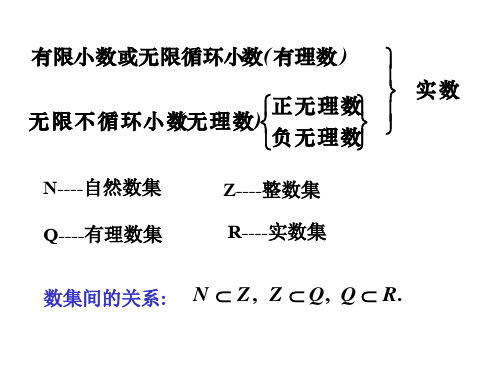
有限小数或无限循环小数( 有理数 )
高等数学-微积分第1章(英文讲稿)

高等数学-微积分第1章(英文讲稿)C alc u lus (Fifth Edition)高等数学- Calculus微积分(双语讲稿)Chapter 1 Functions and Models1.1 Four ways to represent a function1.1.1 ☆Definition(1-1) function: A function f is a rule that assigns to each element x in a set A exactly one element, called f(x), in a set B. see Fig.2 and Fig.3Conceptions: domain; range (See fig. 6 p13); independent variable; dependent variable. Four possible ways to represent a function: 1)Verbally语言描述(by a description in words); 2) Numerically数据表述(by a table of values); 3) Visually 视觉图形描述(by a graph);4)Algebraically 代数描述(by an explicit formula).1.1.2 A question about a Curve represent a function and can’t represent a functionThe way ( The vertical line test ) : A curve in the xy-plane is the graph of a function of x if and only if no vertical line intersects the curve more than once. See Fig.17 p 171.1.3 ☆Piecewise defined functions (分段定义的函数)Example7 (P18)1-x if x ≤1f(x)=﹛x2if x>1Evaluate f(0),f(1),f(2) and sketch the graph.Solution:1.1.4 About absolute value (分段定义的函数)⑴∣x∣≥0;⑵∣x∣≤0Example8 (P19)Sketch the graph of the absolute value function f(x)=∣x∣.Solution:1.1.5☆☆Symmetry ,(对称) Even functions and Odd functions (偶函数和奇函数)⑴Symmetry See Fig.23 and Fig.24⑵①Even functions: If a function f satisfies f(-x)=f(x) for every number x in its domain,then f is call an even function. Example f(x)=x2 is even function because: f(-x)= (-x)2=x2=f(x)②Odd functions: If a function f satisfie s f(-x)=-f(x) for every number x in its domain,thenf is call an odd function. Example f(x)=x3 is even function because: f(-x)=(-x)3=-x3=-f(x)③Neither even nor odd functions:1.1.6☆☆Increasing and decreasing function (增函数和减函数)⑴Definition(1-2) increasing and decreasing function:① A function f is called increasing on an interval I if f(x1)<f(x2) whenever x1<x2 in I. ①A function f is called decreasing on an interval I if f(x1)>f(x2) whenever x1<x2 in I.See Fig.26. and Fig.27. p211.2 Mathematical models: a catalog of essential functions p251.2.1 A mathematical model p25A mathematical model is a mathematical description of a real-world phenomenon such as the size of a population, the demand for a product, the speed of a falling object, the concentration of a product in a chemical reaction, the life expectancy of a person at birth, or the cost of emission reduction.1.2.2 Linear models and Linear function P261.2.3 Polynomial P27A function f is called a polynomial ifP(x) =a n x n+a n-1x n-1+…+a2x2+a1x+a0Where n is a nonnegative integer and the numbers a0,a1,a2,…,a n-1,a n are constants called the coefficients of the polynomial. The domain of any polynomial is R=(-∞,+∞).if the leading coefficient a n≠0, then the degree of the polynomial is n. For example, the function P(x) =5x6+2x5-x4+3x-9⑴Quadratic function example: P(x) =5x2+2x-3 二次函数(方程)⑵Cubic function example: P(x) =6x3+3x2-1 三次函数(方程)1.2.4Power functions幂函数P30A function of the form f(x) =x a,Where a is a constant, is called a power function. We consider several cases:⑴a=n where n is a positive integer ,(n=1,2,3,…,)⑵a=1/n where n is a positive integer,(n=1,2,3,…,) The function f(x) =x1/n⑶a=n-1 the graph of the reciprocal function f(x) =x-1 反比函数1.2.5Rational function有理函数P 32A rational function f is a ratio of two polynomials:f(x)=P(x) /Q(x)1.2.6Algebraic function代数函数P32A function f is called algebraic function if it can be constructed using algebraic operations ( such as addition,subtraction,multiplication,division,and taking roots) starting with polynomials. Any rational function is automatically an algebraic function. Examples: P 321.2.7Trigonometric functions 三角函数P33⑴f(x)=sin x⑵f(x)=cos x⑶f(x)=tan x=sin x / cos x1.2.8Exponential function 指数函数P34The exponential functions are the functions the form f(x) =a x Where the base a is a positive constant.1.2.9Transcendental functions 超越函数P35These are functions that are not a algebraic. The set of transcendental functions includes the trigonometric,inverse trigonometric,exponential,and logarithmic functions,but it also includes a vast number of other functions that have never been named. In Chapter 11 we will study transcendental functions that are defined as sums of infinite series.1.2 Exercises P 35-381.3 New functions from old functions1.3.1 Transformations of functions P38⑴Vertical and Horizontal shifts (See Fig.1 p39)①y=f(x)+c,(c>0)shift the graph of y=f(x) a distance c units upward.②y=f(x)-c,(c>0)shift the graph of y=f(x) a distance c units downward.③y=f(x+c),(c>0)shift the graph of y=f(x) a distance c units to the left.④y=f(x-c),(c>0)shift the graph of y=f(x) a distance c units to the right.⑵ V ertical and Horizontal Stretching and Reflecting (See Fig.2 p39)①y=c f(x),(c>1)stretch the graph of y=f(x) vertically bya factor of c②y=(1/c) f(x),(c>1)compress the graph of y=f(x) vertically by a factor of c③y=f(x/c),(c>1)stretch the graph of y=f(x) horizontally by a factor of c.④y=f(c x),(c>1)compress the graph of y=f(x) horizontally by a factor of c.⑤y=-f(x),reflect the graph of y=f(x) about the x-axis⑥y=f(-x),reflect the graph of y=f(x) about the y-axisExamples1: (See Fig.3 p39)y=f( x) =cos x,y=f( x) =2cos x,y=f( x) =(1/2)cos x,y=f( x) =cos(x/2),y=f( x) =cos2xExamples2: (See Fig.4 p40)Given the graph y=f( x) =( x)1/2,use transformations to graph y=f( x) =( x)1/2-2,y=f( x) =(x-2)1/2,y=f( x) =-( x)1/2,y=f( x) =2 ( x)1/2,y=f( x) =(-x)1/21.3.2 Combinations of functions (代数组合函数)P42Algebra of functions: Two functions (or more) f and g through the way such as add, subtract, multiply and divide to combined a new function called Combination of function.☆Definition(1-2) Combination function: Let f and g be functions with domains A and B. The functions f±g,f g and f /g are defined as follows: (特别注意符号(f±g)( x) 定义的含义)①(f±g)( x)=f(x)±g( x),domain =A∩B②(f g)( x)=f(x) g( x),domain =A∩ B③(f /g)( x)=f(x) /g( x),domain =A∩ B and g( x)≠0Example 6 If f( x) =( x)1/2,and g( x)=(4-x2)1/2,find functions y=f(x)+g( x),y=f(x)-g( x),y=f(x)g( x),and y=f(x) /g( x)Solution: The domain of f( x) =( x)1/2 is [0,+∞),The domain of g( x) =(4-x2)1/2 is interval [-2,2],The intersection of the domains of f(x) and g( x) is[0,+∞)∩[-2,2]=[0,2]Thus,according to the definitions, we have(f+g)( x)=( x)1/2+(4-x2)1/2,domain [0,2](f-g)( x)=( x)1/2-(4-x2)1/2,domain [0,2](f g)( x)=f(x) g( x) =( x)1/2(4-x2)1/2=(4 x-x3)1/2domain [0,2](f /g)( x)=f(x)/g( x)=( x)1/2/(4-x2)1/2=[ x/(4-x2)]1/2 domain [0,2)1.3.3☆☆Composition of functions (复合函数)P45☆Definition(1-3) Composition function: Given two functions f and g the composite func tion f⊙g (also called the composition of f and g ) is defined by(f⊙g)( x)=f( g( x)) (特别注意符号(f⊙g)( x) 定义的含义)The domain of f⊙g is the set of all x in the domain of g such that g(x) is in the domain of f . In other words, (f⊙g)(x) is defined whenever both g(x) and f (g (x)) are defined. See Fig.13 p 44 Example7 If f (g)=( g)1/2 and g(x)=(4-x3)1/2find composite functions f⊙g and g⊙f Solution We have(f⊙g)(x)=f (g (x) ) =( g)1/2=((4-x3)1/2)1/2(g⊙f)(x)=g (f (x) )=(4-x3)1/2=[4-((x)1/2)3]1/2=[4-(x)3/2]1/2Example8 If f (x)=( x)1/2 and g(x)=(2-x)1/2find composite function s①f⊙g ②g⊙f ③f⊙f④g⊙gSolution We have①f⊙g=(f⊙g)(x)=f (g (x) )=f((2-x)1/2)=((2-x)1/2)1/2=(2-x)1/4The domain of (f⊙g)(x) is 2-x≥0 that is x ≤2 {x ︳x ≤2 }=(-∞,2]②g⊙f=(g⊙f)(x)=g (f (x) )=g (( x)1/2 )=(2-( x)1/2)1/2The domain of (g⊙f)(x) is x≥0 and 2-( x)1/2x ≥0 ,that is( x)1/2≤2 ,or x ≤ 4 ,so the domain of g⊙f is the closed interval[0,4]③f⊙f=(f⊙f)(x)=f (f(x) )=f((x)1/2)=((x)1/2)1/2=(x)1/4The domain of (f⊙f)(x) is [0,∞)④g⊙g=(g⊙g)(x)=g (g(x) )=g ((2-x)1/2 )=(2-(2-x)1/2)1/2The domain of (g⊙g)(x) is x-2≥0 and 2-(2-x)1/2≥0 ,that is x ≤2 and x ≥-2,so the domain of g⊙g is the closed interval[-2,2]Notice: g⊙f⊙h=f (g(h(x)))Example9Example10 Given F (x)=cos2( x+9),find functions f,g,and h such that F (x)=f⊙g⊙h Solution Since F (x)=[cos ( x+9)] 2,that is h (x)=x+9 g(x)=cos x f (x)=x2Exercise P 45-481.4 Graphing calculators and computers P481.5 Exponential functions⑴An exponential function is a function of the formf (x)=a x See Fig.3 P56 and Fig.4Exponential functions increasing and decreasing (单调性讨论)⑵Lows of exponents If a and b are positive numbers and x and y are any real numbers. Then1) a x+y=a x a y2) a x-y=a x / a y3) (a x)y=a xy4) (ab)x+y =a x b x⑶about the number e f (x)=e x See Fig. 14,15 P61Some of the formulas of calculus will be greatly simplified if we choose the base a .Exercises P 62-631.6 Inverse functions and logarithms1.6.1 Definition(1-4) one-to-one function: A function f iscalled a one-to-one function if it never takes on the same value twice;that is,f (x1)≠f (x2),whenever x1≠x2( 注解:不同的自变量一定有不同的函数值,不同的自变量有相同的函数值则不是一一对应函数) Example: f (x)=x3is one-to-one function.f (x)=x2 is not one-to-one function, See Fig.2,3,4 ☆☆Definition(1-5) Inverse function:Let f be a one-to-one function with domain A and range B. Then its inverse function f -1(y)has domain B and range A and is defined byf-1(y)=x f (x)=y for any y in Bdomain of f-1=range of frange of f-1=domain of f( 注解:it says : if f maps x into y, then f-1maps y back into x . Caution: If f were not one-to-one function,then f-1 would not be uniquely defined. )Caution: Do not mistake the-1 in f-1for an exponent. Thus f-1(x)=1/ f(x) Because the letter x is traditionally used as the independent variable, so when we concentrate on f-1(y) rather than on f-1(y), we usually reverse the roles of x and y in Definition (1-5) and write as f-1(x)=y f (x)=yWe get the following cancellation equations:f-1( f(x))=x for every x in Af (f-1(x))=x for every x in B See Fig.7 P66Example 4 Find the inverse function of f(x)=x3+6Solution We first writef(x)=y=x3+6Then we solve this equation for x:x3=y-6x=(y-6)1/3Finally, we interchange x and y:y=(x-6)1/3That is, the inverse function is f-1(x)=(x-6)1/3( 注解:The graph of f-1 is obtained by reflecting the graph of f about the line y=x. ) See Fig.9、8 1.6.2 Logarithmic function If a>0 and a≠1,the exponential function f (x)=a x is either increasing or decreasing and so it is one-to-one function by the Horizontal Line Test. It therefore has an inverse function f-1,which is called the logarithmic function with base a and is denoted log a,If we use the formulation of an inverse function given by (See Fig.3 P56)f-1(x)=y f (x)=yThen we havelogx=y a y=xThe logarithmic function log a x=y has domain (0,∞) and range R.Usefully equations:①log a(a x)=x for every x∈R②a log ax=x for every x>01.6.3 ☆Lows of logarithms :If x and y are positive numbers, then①log a(xy)=log a x+log a y②log a(x/y)=log a x-log a y③log a(x)r=r log a x where r is any real number1.6.4 Natural logarithmsNatural logarithm isl og e x=ln x =ythat is①ln x =y e y=x② ln(e x)=x x∈R③e ln x=x x>0 ln e=1Example 8 Solve the equation e5-3x=10Solution We take natural logarithms of both sides of the equation and use ②、③ln (e5-3x)=ln10∴5-3x=ln10x=(5-ln10)/3Example 9 Express ln a+(ln b)/2 as a single logarithm.Solution Using laws of logarithms we have:ln a+(ln b)/2=ln a+ln b1/2=ln(ab1/2)1.6.5 ☆Change of Base formula For any positive number a (a≠1), we havel og a x=ln x/ ln a1.6.6 Inverse trigonometric functions⑴Inverse sine function or Arcsine functionsin-1x=y sin y=x and -π/2≤y≤π / 2,-1≤x≤1 See Fig.18、20 P72Example13 ① sin-1 (1/2) or arcsin(1/2) ② tan(arcsin1/3)Solution①∵sin (π/6)=1/2,π/6 lies between -π/2 and π / 2,∴sin-1 (1/2)=π/6② Let θ=arcsin1/3,so sinθ=1/3tan(arcsin1/3)=tanθ=s inθ/cosθ=(1/3)/(1-s in2θ)1/2=1/(8)1/2Usefully equations:①sin-1(sin x)=x for -π/2≤x≤π / 2②sin (sin-1x)=x for -1≤x≤1⑵Inverse cosine function or Arccosine functioncos-1x=y cos y=x and 0 ≤y≤π,-1≤x≤1 See Fig.21、22 P73Usefully equations:①cos-1(cos x)=x for 0 ≤x≤π②cos (cos-1x)=x for -1≤x≤1⑶Inverse Tangent function or Arctangent functiontan-1x=y tan y=x and -π/2<y<π / 2 ,x∈R See Fig.23 P73、Fig.25 P74Example 14 Simplify the expression cos(ta n-1x).Solution 1 Let y=tan-1 x,Then tan y=x and -π/2<y<π / 2 ,We want find cos y but since tan y is known, it is easier to find sec y first:sec2y=1 +tan2y sec y=(1 +x2 )1/2∴cos(ta n-1x)=cos y =1/ sec y=(1 +x2)-1/2Solution 2∵cos(ta n-1x)=cos y∴cos(ta n-1x)=(1 +x2)-1/2⑷Other Inverse trigonometric functionscsc-1x=y∣x∣≥1csc y=x and y∈(0,π / 2]∪(π,3π / 2]sec-1x=y∣x∣≥1sec y=x and y∈[0,π / 2)∪[π,3π / 2]cot-1x=y x∈R cot y=x and y∈(0,π)Exercises P 74-85Key words and PhrasesCalculus 微积分学Set 集合Variable 变量Domain 定义域Range 值域Arbitrary number 独立变量Independent variable 自变量Dependent variable 因变量Square root 平方根Curve 曲线Interval 区间Interval notation 区间符号Closed interval 闭区间Opened interval 开区间Absolute 绝对值Absolute value 绝对值Symmetry 对称性Represent of a function 函数的表述(描述)Even function 偶函数Odd function 奇函数Increasing Function 增函数Increasing Function 减函数Empirical model 经验模型Essential Function 基本函数Linear function 线性函数Polynomial function 多项式函数Coefficient 系数Degree 阶Quadratic function 二次函数(方程)Cubic function 三次函数(方程)Power functions 幂函数Reciprocal function 反比函数Rational function 有理函数Algebra 代数Algebraic function 代数函数Integer 整数Root function 根式函数(方程)Trigonometric function 三角函数Exponential function 指数函数Inverse function 反函数Logarithm function 对数函数Inverse trigonometric function 反三角函数Natural logarithm function 自然对数函数Chang of base of formula 换底公式Transcendental function 超越函数Transformations of functions 函数的变换Vertical shifts 垂直平移Horizontal shifts 水平平移Stretch 伸张Reflect 反演Combinations of functions 函数的组合Composition of functions 函数的复合Composition function 复合函数Intersection 交集Quotient 商Arithmetic 算数。
微积分第一章第一节课件

微积分作为数学的基础学科,对于理解数学的高级概念和解决复杂问题具有重要意义。同时,它在物理学、工程 学、经济学等多个领域都有广泛的应用。
教学目标
知识与技能
情感态度与价值观
通过本课程的学习,学生应掌握微积 分的基本概念、基本理论和基本方法, 具备运用微积分知识解决实际问题的 能力。
培养学生严谨的数学思维习惯,激发 学生对数学的兴趣和热爱,树立正确 的数学价值观。
广义积分与含参变量积分
广义积分
广义积分是对定积分的扩展,包括无穷 限广义积分和无界函数广义积分两种类 型。广义积分的计算需要借助极限的思 想和方法。
VS
含参变量积分
含参变量积分是一种特殊的定积分,其被 积函数中含有参数。含参变量积分的计算 方法和性质与定积分类似,但需要注意参 数的影响。同时,含参变量积分在实际问 题中有着广泛的应用,如概率论、统计学 等领域。
定积分性质
定积分具有线性性、可加性、保号性、 绝对值不等式、积分中值定理等基本 性质。
不定积分概念及计算法则
不定积分概念
不定积分是微分学的逆运算,其结果是一个函数族。不定积分的定义包括被积函数、积分变量和常数 C等要素。
不定积分计算法则
不定积分的计算法则包括基本积分公式、换元积分法、分部积分法等。其中,基本积分公式是计算不 定积分的基础,换元积分法和分部积分法是常用的计算技巧。
微积分在实际问题中的应用
探讨微积分在物理、经济、工程等领域的实际应 用,如求解最值问题、分析物理现象等。
3
微积分的数值计算方法
研究微积分的数值计算方法,如有限差分法、有 限元法等,为实际应用提供有效的数值求解工具。
课后作业布置
01
02
微积分专题讲座讲义
d dy dy 2 dy dt d y dt dx ) 公式法) ;⑷参数方程确定的函数(用导数公式: , 2 ;⑸抽象函数(正确使用导数记 dx dx dx dx dt dt
号,注意 f ( x ) 和 [ f ( x )] 的区别) ;⑹幂指函数(对数求导法) ;⑺反函数(导数公式:
2 0
f (sin x)dx ;
▲记 I n
2 0
sin n xdx 2 cos n xdx ,则有递推公式 I n
0
n 1 I n2 . n
⑤含 f , f (用分部积分) ⑥变限积分(用分部积分) 若 f ( x) 在 [ a, b] 上连续,则 ( x) 公式
x a
f (t )dt 在 [a, b] 上可导,且 x [a, b] , ( x) f ( x) .
d b d ( x) f (t )dt f ( x) ; f (t )dt f ( ( x)) ( x) ; dx x dx a d ( x) f (t )dt f ( ( x)) ( x) f ( ( x)) ( x) dx ( x ) ▲当被积函数含变量 x 时不能直接求导, 必须将变量 x 从被积函数中分离出去, 常用的方法是: 提出去或者换元.
【- 4 -】
一、一阶微分方程 一阶微分方程的一般形式是: F ( x, y, y) 0 ,解出 y :
dy f ( x, y ) ,要求掌握变量可分离的微分方程、一阶 dx
线性微分方程、.齐次微分方程、伯努利方程的解法. 求解微分方程的步骤是:判断方程的类型并用相应的方法求解. 二、可降阶的微分方程 1. y f ( x) 型的微分方程 特点:右端仅含 x .解法:积分两次. 2. y f ( x, y) 型的微分方程 特点:右端不显含未知函数 y .解法:换元,化为一阶方程求解. 步骤如下: ⑴令 y p ,则 y
高等数学-微积分第1章(英文讲稿)
C alc u lus (Fifth Edition)高等数学- Calculus微积分(双语讲稿)Chapter 1 Functions and Models1.1 Four ways to represent a function1.1.1 ☆Definition(1-1) function: A function f is a rule that assigns to each element x in a set A exactly one element, called f(x), in a set B. see Fig.2 and Fig.3Conceptions: domain; range (See fig. 6 p13); independent variable; dependent variable. Four possible ways to represent a function: 1)Verbally语言描述(by a description in words); 2) Numerically数据表述(by a table of values); 3) Visually 视觉图形描述(by a graph);4)Algebraically 代数描述(by an explicit formula).1.1.2 A question about a Curve represent a function and can’t represent a functionThe way ( The vertical line test ) : A curve in the xy-plane is the graph of a function of x if and only if no vertical line intersects the curve more than once. See Fig.17 p 171.1.3 ☆Piecewise defined functions (分段定义的函数)Example7 (P18)1-x if x ≤1f(x)=﹛x2if x>1Evaluate f(0),f(1),f(2) and sketch the graph.Solution:1.1.4 About absolute value (分段定义的函数)⑴∣x∣≥0;⑵∣x∣≤0Example8 (P19)Sketch the graph of the absolute value function f(x)=∣x∣.Solution:1.1.5☆☆Symmetry ,(对称) Even functions and Odd functions (偶函数和奇函数)⑴Symmetry See Fig.23 and Fig.24⑵①Even functions: If a function f satisfies f(-x)=f(x) for every number x in its domain,then f is call an even function. Example f(x)=x2 is even function because: f(-x)= (-x)2=x2=f(x)②Odd functions: If a function f satisfies f(-x)=-f(x) for every number x in its domain,thenf is call an odd function. Example f(x)=x3 is even function because: f(-x)=(-x)3=-x3=-f(x)③Neither even nor odd functions:1.1.6☆☆Increasing and decreasing function (增函数和减函数)⑴Definition(1-2) increasing and decreasing function:① A function f is called increasing on an interval I if f(x1)<f(x2) whenever x1<x2 in I. ①A function f is called decreasing on an interval I if f(x1)>f(x2) whenever x1<x2 in I.See Fig.26. and Fig.27. p211.2 Mathematical models: a catalog of essential functions p251.2.1 A mathematical model p25A mathematical model is a mathematical description of a real-world phenomenon such as the size of a population, the demand for a product, the speed of a falling object, the concentration of a product in a chemical reaction, the life expectancy of a person at birth, or the cost of emission reduction.1.2.2 Linear models and Linear function P261.2.3 Polynomial P27A function f is called a polynomial ifP(x) =a n x n+a n-1x n-1+…+a2x2+a1x+a0Where n is a nonnegative integer and the numbers a0,a1,a2,…,a n-1,a n are constants called the coefficients of the polynomial. The domain of any polynomial is R=(-∞,+∞).if the leading coefficient a n≠0, then the degree of the polynomial is n. For example, the function P(x) =5x6+2x5-x4+3x-9⑴Quadratic function example: P(x) =5x2+2x-3 二次函数(方程)⑵Cubic function example: P(x) =6x3+3x2-1 三次函数(方程)1.2.4Power functions幂函数P30A function of the form f(x) =x a,Where a is a constant, is called a power function. We consider several cases:⑴a=n where n is a positive integer ,(n=1,2,3,…,)⑵a=1/n where n is a positive integer,(n=1,2,3,…,) The function f(x) =x1/n⑶a=n-1 the graph of the reciprocal function f(x) =x-1 反比函数1.2.5Rational function有理函数P 32A rational function f is a ratio of two polynomials:f(x)=P(x) /Q(x)1.2.6Algebraic function代数函数P32A function f is called algebraic function if it can be constructed using algebraic operations ( such as addition,subtraction,multiplication,division,and taking roots) starting with polynomials. Any rational function is automatically an algebraic function. Examples: P 321.2.7Trigonometric functions 三角函数P33⑴f(x)=sin x⑵f(x)=cos x⑶f(x)=tan x=sin x / cos x1.2.8Exponential function 指数函数P34The exponential functions are the functions the form f(x) =a x Where the base a is a positive constant.1.2.9Transcendental functions 超越函数P35These are functions that are not a algebraic. The set of transcendental functions includes the trigonometric,inverse trigonometric,exponential,and logarithmic functions,but it also includes a vast number of other functions that have never been named. In Chapter 11 we will study transcendental functions that are defined as sums of infinite series.1.2 Exercises P 35-381.3 New functions from old functions1.3.1 Transformations of functions P38⑴Vertical and Horizontal shifts (See Fig.1 p39)①y=f(x)+c,(c>0)shift the graph of y=f(x) a distance c units upward.②y=f(x)-c,(c>0)shift the graph of y=f(x) a distance c units downward.③y=f(x+c),(c>0)shift the graph of y=f(x) a distance c units to the left.④y=f(x-c),(c>0)shift the graph of y=f(x) a distance c units to the right.⑵ V ertical and Horizontal Stretching and Reflecting (See Fig.2 p39)①y=c f(x),(c>1)stretch the graph of y=f(x) vertically by a factor of c②y=(1/c) f(x),(c>1)compress the graph of y=f(x) vertically by a factor of c③y=f(x/c),(c>1)stretch the graph of y=f(x) horizontally by a factor of c.④y=f(c x),(c>1)compress the graph of y=f(x) horizontally by a factor of c.⑤y=-f(x),reflect the graph of y=f(x) about the x-axis⑥y=f(-x),reflect the graph of y=f(x) about the y-axisExamples1: (See Fig.3 p39)y=f( x) =cos x,y=f( x) =2cos x,y=f( x) =(1/2)cos x,y=f( x) =cos(x/2),y=f( x) =cos2xExamples2: (See Fig.4 p40)Given the graph y=f( x) =( x)1/2,use transformations to graph y=f( x) =( x)1/2-2,y=f( x) =(x-2)1/2,y=f( x) =-( x)1/2,y=f( x) =2 ( x)1/2,y=f( x) =(-x)1/21.3.2 Combinations of functions (代数组合函数)P42Algebra of functions: Two functions (or more) f and g through the way such as add, subtract, multiply and divide to combined a new function called Combination of function.☆Definition(1-2) Combination function: Let f and g be functions with domains A and B. The functions f±g,f g and f /g are defined as follows: (特别注意符号(f±g)( x) 定义的含义)①(f±g)( x)=f(x)±g( x),domain =A∩B②(f g)( x)=f(x) g( x),domain =A∩ B③(f /g)( x)=f(x) /g( x),domain =A∩ B and g( x)≠0Example 6 If f( x) =( x)1/2,and g( x)=(4-x2)1/2,find functions y=f(x)+g( x),y=f(x)-g( x),y=f(x)g( x),and y=f(x) /g( x)Solution: The domain of f( x) =( x)1/2 is [0,+∞),The domain of g( x) =(4-x2)1/2 is interval [-2,2],The intersection of the domains of f(x) and g( x) is[0,+∞)∩[-2,2]=[0,2]Thus,according to the definitions, we have(f+g)( x)=( x)1/2+(4-x2)1/2,domain [0,2](f-g)( x)=( x)1/2-(4-x2)1/2,domain [0,2](f g)( x)=f(x) g( x) =( x)1/2(4-x2)1/2=(4 x-x3)1/2domain [0,2](f /g)( x)=f(x)/g( x)=( x)1/2/(4-x2)1/2=[ x/(4-x2)]1/2 domain [0,2)1.3.3☆☆Composition of functions (复合函数)P45☆Definition(1-3) Composition function: Given two functions f and g the composite function f⊙g (also called the composition of f and g ) is defined by(f⊙g)( x)=f( g( x)) (特别注意符号(f⊙g)( x) 定义的含义)The domain of f⊙g is the set of all x in the domain of g such that g(x) is in the domain of f . In other words, (f⊙g)(x) is defined whenever both g(x) and f (g (x)) are defined. See Fig.13 p 44 Example7 If f (g)=( g)1/2 and g(x)=(4-x3)1/2find composite functions f⊙g and g⊙f Solution We have(f⊙g)(x)=f (g (x) ) =( g)1/2=((4-x3)1/2)1/2(g⊙f)(x)=g (f (x) )=(4-x3)1/2=[4-((x)1/2)3]1/2=[4-(x)3/2]1/2Example8 If f (x)=( x)1/2 and g(x)=(2-x)1/2find composite function s①f⊙g ②g⊙f ③f⊙f④g⊙gSolution We have①f⊙g=(f⊙g)(x)=f (g (x) )=f((2-x)1/2)=((2-x)1/2)1/2=(2-x)1/4The domain of (f⊙g)(x) is 2-x≥0 that is x ≤2 {x ︳x ≤2 }=(-∞,2]②g⊙f=(g⊙f)(x)=g (f (x) )=g (( x)1/2 )=(2-( x)1/2)1/2The domain of (g⊙f)(x) is x≥0 and 2-( x)1/2x ≥0 ,that is ( x)1/2≤2 ,or x ≤ 4 ,so the domain of g⊙f is the closed interval[0,4]③f⊙f=(f⊙f)(x)=f (f(x) )=f((x)1/2)=((x)1/2)1/2=(x)1/4The domain of (f⊙f)(x) is [0,∞)④g⊙g=(g⊙g)(x)=g (g(x) )=g ((2-x)1/2 )=(2-(2-x)1/2)1/2The domain of (g⊙g)(x) is x-2≥0 and 2-(2-x)1/2≥0 ,that is x ≤2 and x ≥-2,so the domain of g⊙g is the closed interval[-2,2]Notice: g⊙f⊙h=f (g(h(x)))Example9Example10 Given F (x)=cos2( x+9),find functions f,g,and h such that F (x)=f⊙g⊙h Solution Since F (x)=[cos ( x+9)] 2,that is h (x)=x+9 g(x)=cos x f (x)=x2Exercise P 45-481.4 Graphing calculators and computers P481.5 Exponential functions⑴An exponential function is a function of the formf (x)=a x See Fig.3 P56 and Fig.4Exponential functions increasing and decreasing (单调性讨论)⑵Lows of exponents If a and b are positive numbers and x and y are any real numbers. Then1) a x+y=a x a y2) a x-y=a x / a y3) (a x)y=a xy4) (ab)x+y=a x b x⑶about the number e f (x)=e x See Fig. 14,15 P61Some of the formulas of calculus will be greatly simplified if we choose the base a .Exercises P 62-631.6 Inverse functions and logarithms1.6.1 Definition(1-4) one-to-one function: A function f is called a one-to-one function if it never takes on the same value twice;that is,f (x1)≠f (x2),whenever x1≠x2( 注解:不同的自变量一定有不同的函数值,不同的自变量有相同的函数值则不是一一对应函数) Example: f (x)=x3is one-to-one function.f (x)=x2 is not one-to-one function, See Fig.2,3,4☆☆Definition(1-5) Inverse function:Let f be a one-to-one function with domain A and range B. Then its inverse function f-1(y)has domain B and range A and is defined byf-1(y)=x f (x)=y for any y in Bdomain of f-1=range of frange of f-1=domain of f( 注解:it says : if f maps x into y, then f-1maps y back into x . Caution: If f were not one-to-one function,then f-1 would not be uniquely defined. )Caution: Do not mistake the-1 in f-1for an exponent. Thus f-1(x)=1/ f(x) !!!Because the letter x is traditionally used as the independent variable, so when we concentrate on f-1(y) rather than on f-1(y), we usually reverse the roles of x and y in Definition (1-5) and write as f-1(x)=y f (x)=yWe get the following cancellation equations:f-1( f(x))=x for every x in Af (f-1(x))=x for every x in B See Fig.7 P66Example 4 Find the inverse function of f(x)=x3+6Solution We first writef(x)=y=x3+6Then we solve this equation for x:x3=y-6x=(y-6)1/3Finally, we interchange x and y:y=(x-6)1/3That is, the inverse function is f-1(x)=(x-6)1/3( 注解:The graph of f-1 is obtained by reflecting the graph of f about the line y=x. ) See Fig.9、8 1.6.2 Logarithmic functionIf a>0 and a≠1,the exponential function f (x)=a x is either increasing or decreasing and so it is one-to-one function by the Horizontal Line Test. It therefore has an inverse function f-1,which is called the logarithmic function with base a and is denoted log a,If we use the formulation of an inverse function given by (See Fig.3 P56)f-1(x)=y f (x)=yThen we havelogx=y a y=xThe logarithmic function log a x=y has domain (0,∞) and range R.Usefully equations:①log a(a x)=x for every x∈R②a log ax=x for every x>01.6.3 ☆Lows of logarithms :If x and y are positive numbers, then①log a(xy)=log a x+log a y②log a(x/y)=log a x-log a y③log a(x)r=r log a x where r is any real number1.6.4 Natural logarithmsNatural logarithm isl og e x=ln x =ythat is①ln x =y e y=x② ln(e x)=x x∈R③e ln x=x x>0 ln e=1Example 8 Solve the equation e5-3x=10Solution We take natural logarithms of both sides of the equation and use ②、③ln (e5-3x)=ln10∴5-3x=ln10x=(5-ln10)/3Example 9 Express ln a+(ln b)/2 as a single logarithm.Solution Using laws of logarithms we have:ln a+(ln b)/2=ln a+ln b1/2=ln(ab1/2)1.6.5 ☆Change of Base formula For any positive number a (a≠1), we havel og a x=ln x/ ln a1.6.6 Inverse trigonometric functions⑴Inverse sine function or Arcsine functionsin-1x=y sin y=x and -π/2≤y≤π / 2,-1≤x≤1 See Fig.18、20 P72Example13 ① sin-1 (1/2) or arcsin(1/2) ② tan(arcsin1/3)Solution①∵sin (π/6)=1/2,π/6 lies between -π/2 and π / 2,∴sin-1 (1/2)=π/6② Let θ=arcsin1/3,so sinθ=1/3tan(arcsin1/3)=tanθ= s inθ/cosθ= (1/3)/(1-s in2θ)1/2=1/(8)1/2Usefully equations:①sin-1(sin x)=x for -π/2≤x≤π / 2②sin (sin-1x)=x for -1≤x≤1⑵Inverse cosine function or Arccosine functioncos-1x=y cos y=x and 0 ≤y≤π,-1≤x≤1 See Fig.21、22 P73Usefully equations:①cos-1(cos x)=x for 0 ≤x≤π②cos (cos-1x)=x for -1≤x≤1⑶Inverse Tangent function or Arctangent functiontan-1x=y tan y=x and -π/2<y<π / 2 ,x∈R See Fig.23 P73、Fig.25 P74Example 14 Simplify the expression cos(ta n-1x).Solution 1 Let y=tan-1 x,Then tan y=x and -π/2<y<π / 2 ,We want find cos y but since tan y is known, it is easier to find sec y first:sec2y=1 +tan2y sec y=(1 +x2 )1/2∴cos(ta n-1x)=cos y =1/ sec y=(1 +x2)-1/2Solution 2∵cos(ta n-1x)=cos y∴cos(ta n-1x)=(1 +x2)-1/2⑷Other Inverse trigonometric functionscsc-1x=y∣x∣≥1csc y=x and y∈(0,π / 2]∪(π,3π / 2]sec-1x=y∣x∣≥1sec y=x and y∈[0,π / 2)∪[π,3π / 2]cot-1x=y x∈R cot y=x and y∈(0,π)Exercises P 74-85Key words and PhrasesCalculus 微积分学Set 集合Variable 变量Domain 定义域Range 值域Arbitrary number 独立变量Independent variable 自变量Dependent variable 因变量Square root 平方根Curve 曲线Interval 区间Interval notation 区间符号Closed interval 闭区间Opened interval 开区间Absolute 绝对值Absolute value 绝对值Symmetry 对称性Represent of a function 函数的表述(描述)Even function 偶函数Odd function 奇函数Increasing Function 增函数Increasing Function 减函数Empirical model 经验模型Essential Function 基本函数Linear function 线性函数Polynomial function 多项式函数Coefficient 系数Degree 阶Quadratic function 二次函数(方程)Cubic function 三次函数(方程)Power functions 幂函数Reciprocal function 反比函数Rational function 有理函数Algebra 代数Algebraic function 代数函数Integer 整数Root function 根式函数(方程)Trigonometric function 三角函数Exponential function 指数函数Inverse function 反函数Logarithm function 对数函数Inverse trigonometric function 反三角函数Natural logarithm function 自然对数函数Chang of base of formula 换底公式Transcendental function 超越函数Transformations of functions 函数的变换Vertical shifts 垂直平移Horizontal shifts 水平平移Stretch 伸张Reflect 反演Combinations of functions 函数的组合Composition of functions 函数的复合Composition function 复合函数Intersection 交集Quotient 商Arithmetic 算数。
五分钟MIT公开课

五分钟MIT公开课简介从上一篇开始,我们就正式开始线积分的学习了。
初学线积分的人可能会感觉到畏惧与头疼,因为线积分的知识点非常繁杂。
MIT公开课从物理学角度入手,带给我们最直觉和直观的感受。
另外我也准备了大量的动画帮助理解让线积分不再成为微积分中的拦路虎。
回顾上一篇的知识点,非常重要,其他的比如二重积分都可以暂时扔到一边了。
五分钟MIT公开课-多元微积分:向量场和线积分目录•简介•一个做功的例子•线积分的基本定理•保守和路径独立例子:功的线积分线积分是从物理学的角度引入的,这一节是对物理做功和线积分的回顾。
平面上有一曲线C,有一向量场来描述每一个点上的向量,我们要找出沿着这条曲线所做的功:三个公式分别为定义式,几何表达式和直角坐标系下表达式。
例:在向量场yi+xj里,质点沿一扇形轨迹运动,扇形轨迹由三部分构成。
要计算这个线积分,只要三段分别求和再相加就可以了。
c1:从(0,0) 到(1,0),y=0, dy=0c2:单位圆的一部分。
根据圆的参数方程:c3:参数化这条路径:更简单的表达,使用c3的反向路径:总功:线积分的基本定理算了半天居然是0!怎么能够避免计算?找到这个诀窍,会方便很多。
当多元方程存在的时候,就有梯度向量。
但实际上,是一个向量场。
在这种特殊情况下,向量场实际上是一个函数的梯度,也就是梯度场。
f是关于x和y的函数,称为向量场的势函数(potential)。
在物理学中,计算重力或者电场所做的功,只需要计算起点和终点的势能差,与路径无关。
一个微积分的基本定理是,如果对函数的导数积分,就可以得到原函数。
多元微积分也一样,如果对函数的梯度做线积分,也可以得到原函数。
基本定理:如果沿轨迹对向量场,即方程的梯度做线积分,其结果为原方程的终点与起点值之差注意:非常有局限性,仅仅在向量场是梯度的情况下才满足。
来看看基本定理的物理和几何解释。
对梯度积分,其实是对函数的导数积分:证明:例子回到最开始的例子,向量场为:图像显示了等高线和向量场的重合,可以看出,向量场垂直于等高线,所以也是梯度。
- 1、下载文档前请自行甄别文档内容的完整性,平台不提供额外的编辑、内容补充、找答案等附加服务。
- 2、"仅部分预览"的文档,不可在线预览部分如存在完整性等问题,可反馈申请退款(可完整预览的文档不适用该条件!)。
- 3、如文档侵犯您的权益,请联系客服反馈,我们会尽快为您处理(人工客服工作时间:9:00-18:30)。
Lecture 1
18.01 Fall 2006
Unit 1: Derivatives
A. What is a derivative?
• Geometric interpretation • Physical interpretation • Important for any measurement (economics, political science, finance, physics, etc.)
Lecture 1: Derivatives, Slope, Velocity, and Rate of Change
Geometric Viewpoint on Derivatives
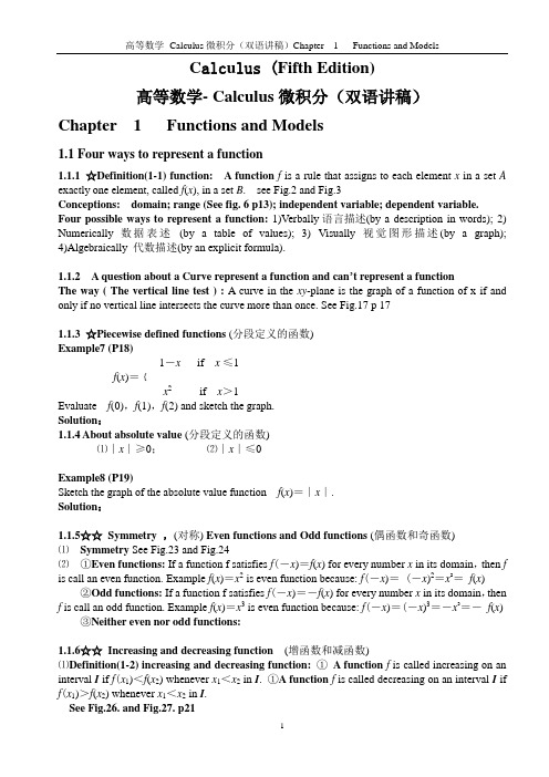
y
Q Secant line P f(x) x0 x0+∆x Tangent line
Figure 1: A function with secant and tangent lines The derivative is the slope of the line tangent to the graph of f (x). But what is a tangent line, exactly? 1
Δx→0
n times
lim
Δy = nxn−1 Δx
Therefore,
d n x = nxn−1 dx This result extends to polynomials. For example, d 2 (x + 3x10 ) = 2x + 30x9 dx
Physical Interpretation of Derivatives
Area = 1 1
(2y0 )(2x0 ) = 2x0 y0 = 2x0 ( ) = 2 (see Fig. 5) 2 x0
Curiously, the area of the triangle is always 2, no matter where on the graph we draw the tangent line.
So, the x-intercept of this tangent line is at x = 2x0 . 1 1 and x = are identical equations, x y the graph is symmetric when x and y are exchanged. By symmetry, then, the y-intercept is at y = 2y0 . If you don’t trust reasoning with symmetry, you may follow the same chain of algebraic reasoning that we used in finding the x-intercept. (Remember, the y-intercept is where x = 0.) Next we claim that the y-intercept is at y = 2y0 . Since y = Finally,
Lecture 1
18.01 Fall 2006
• It is NOT just a line that meets the graph at one point. • It is the limit of the secant line (a line drawn between two points on the graph) as the distance between the two points goes to zero.
P
Байду номын сангаас
∆x
Figure 2: Geometric definition of the derivative
Δx→0
lim
Δf Δx
= lim
Δx→0
“difference quotient”
f (x0 + Δx) − f (x0 ) Δ x � �� �
=
f � (x0 ) � �� � “derivative of f at x0 ”
Example 1. f (x) =
1 x
One thing to keep in mind when working with derivatives: it may be tempting to plug in Δx = 0 Δf 0 right away. If you do this, however, you will always end up with = . You will always need to Δx 0 do some cancellation to get at the answer. Δf = Δx
Δy (x0 + Δx)n − xn (x + Δx)n − xn 0 = = Δx Δx Δx (From here on, we replace x0 with x, so as to have less writing to do.) Since (x + Δx)n = (x + Δx)(x + Δx)...(x + Δx) We can rewrite this as � � xn + n(Δx)xn−1 + O (Δx)2 O(Δx)2 is shorthand for “all of the terms with (Δx)2 , (Δx)3 , and so on up to (Δx)n .” (This is part of what is known as the binomial theorem; see your textbook for details.) Δy (x + Δx)n − xn xn + n(Δx)(xn−1 ) + O(Δx)2 − xn = = = nxn−1 + O(Δx) Δx Δx Δx Take the limit:
MIT OpenCourseWare
18.01 Single Variable Calculus
Fall 2006
For information about citing these materials or our Terms of Use, visit: /terms.
lim
2
Lecture 1
18.01 Fall 2006
y
x0
Figure 3: Graph of Hence,
f � (x0 ) =
1 x
x
−1
x2 0
Notice that f � (x0 ) is negative — as is the slope of the tangent line on the graph above. Finding the tangent line. Write the equation for the tangent line at the point (x0 , y0 ) using the equation for a line, which you all learned in high school algebra: y − y0 = f � (x0 )(x − x0 ) Plug in y0 = f (x0 ) = 1 −1 and f � (x0 ) = 2 to get: x0 x0 y− −1 1 = 2 (x − x0 ) x0 x0
B. How to differentiate any function you know.
d � x arctan x � • For example: e . We will discuss what a derivative is today. Figuring out how to dx differentiate any function is the subject of the first two weeks of this course.
3
Lecture 1
18.01 Fall 2006
y
x0
Figure 4: Graph of
1 x
x
Just for fun, let’s compute the area of the triangle that the tangent line forms with the x- and y-axes (see the shaded region in Fig. 4). First calculate the x-intercept of this tangent line. The x-intercept is where y = 0. Plug y = 0 into the equation for this tangent line to get: 0 − 1 = x0 −1 = x0 1 x = x2 0 x = −1 (x − x0 ) x2 0 −1 1 x+ x2 x 0 0 2 x0 2 x2 ) = 2x0 0( x0
Geometric definition of the derivative:
Limit of slopes of secant lines P Q as Q → P (P fixed). The slope of P Q:
(x0+∆x, f(x0+∆x))
Q
Secant Line
∆f
(x0, f(x0))
When you use Leibniz’ notation, you have to remember where you’re evaluating the derivative — in the example above, at x = x0 . Other, equally valid notations for the derivative of a function f include df � , f , and Df dx