MATLAB作业5 作业本
MATLAB语言基础与应用(第二版)第5章 习题答案
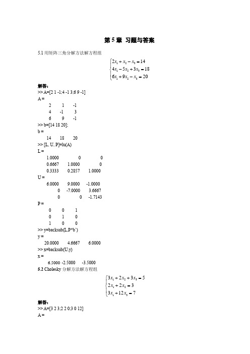
第5章习题与答案5.1用矩阵三角分解方法解方程组123123123214453186920x x x x x x x x x +-=⎧⎪-+=⎨⎪+-=⎩ 解答:>>A=[2 1 -1;4 -1 3;6 9 -1] A =2 1 -1 4 -13 6 9 -1 >>b=[14 18 20]; b =14 18 20 >> [L, U, P]=lu(A) L =1.0000 0 0 0.6667 1.0000 0 0.3333 0.2857 1.0000 U =6.0000 9.0000 -1.0000 0 -7.0000 3.6667 0 0 -1.7143 P =0 0 1 0 1 0 1 0 0 >> y=backsub(L,P*b’) y =20.0000 4.6667 6.0000 >> x=backsub(U,y) x =6.5000 -2.5000 -3.5000 5.2 Cholesky 分解方法解方程组123121332352233127x x x x x x x ++=⎧⎪+=⎨⎪+=⎩ 解答:>> A=[3 2 3;2 2 0;3 0 12] A =3 2 32 2 03 0 12>> b=[5;3;7]b =537>> L=chol(A)L =1.7321 1.1547 1.73210 0.8165 -2.44950 0 1.7321>> y=backsub(L,b)y =-11.6871 15.7986 4.0415>> x=backsub(L',y)x =-6.7475 28.8917 49.93995.3解答:观察数据点图形>> x=0:0.5:2.5x =0 0.5000 1.0000 1.5000 2.0000 2.5000 >> y=[2.0 1.1 0.9 0.6 0.4 0.3]y =2.0000 1.1000 0.9000 0.6000 0.4000 0.3000 >> plot(x,y)图5.1 离散点分布示意图从图5.1观察数据点分布,用二次曲线拟合。
MATLAB第五章作业

第五章作业1.选择题(1)if结构的开始是“if”命令,结束是C命令。
A. End ifB. endC. EndD. else(2)下面的switch结构,正确的是C。
A. >>switch a case a>1B. >>switch acase a=1C. >>switch acase 1D. >>switch acase =1(3)运行以下命令:>>a=eye(5);>>for n=a(2:end,:)则for循环的循环次数是B。
A. 5B. 4C. 3D. 1(4)运行以下命令,则for循环的循环次数是C。
>>x=0:10;>>for n=xif n==5continueendendA. 10B. 5C. 11D. 10(5)运行以下命令则B。
>>a=[1 2 3]>>keyboardK>>a=[1 2 4];K>>returnA. a=[1 2 3]B. a=[1 2 4]C. 命令窗口的提示符为“K>>”D. 出错(6)关于主函数,以下说法正确的是D。
A. 主函数名必须与文件名相同B. 主函数的工作空间与子函数的工作空间是嵌套的C. 主函数中不能定义其他函数D. 每个函数文件中都必须有主函数(7)当在命令窗口中输入“sin(a)”时,则对“a”的搜索顺序是D。
A. 是否内部函数→是否变量→是否私有函数B. 是否内部函数→是否搜索路径中函数→是否私有函数C. 是否内部函数→是否搜索路径中函数→是否当前路径中函数D. 是否变量→是否私有函数→是否当前路径中函数2.求分段函数2226,0356,0<5231x x x xy x x x x xx x⎧+-<≠-⎪=-+≠≠⎨⎪--⎩且≤且及,其他的值。
用if语句实现,分别输出x=-5.0,-3.0,1.0,2.0,2.5,3.0,5.0时的y值。
Matlab上机作业部分参考答案.ppt

[rank(A), rank([A B])]
ans =
34 由得出的结果看,A, [A;B] 两个矩阵的秩不同,故方程是
矛盾方程,没有解。
5. 试求下面齐次方程的基础解系
7. 建立如下一个元胞数组,现在要求计算第一个元胞第4行第 2列加上第二个元胞+第三个元胞里的第二个元素+最后一个元 胞的第二个元素。
a={pascal(4),'hello';17.3500,7:2:100}
解: >> a={pascal(4),'hello';17.3500,7:2:100} a=
[ 173/34, 151/34]
6. 求解方程组的通解
x1 2x2 4x3 6x4 3x5 2x6 4 2x1 4x2 4x3 5x4 x5 5x6 3
3x1 6x2 2x3 5x5 9x6 1 2x1 3x2 4x4 x6 8
4x2
5x3
2x4
x5
参考答案: (1) >> limit(sym('(tan(x) - sin(x))/(1cos(2*x))')) ans = 0 (2) >> y = sym('x^3 - 2*x^2 + sin(x)'); >> diff(y) ans = 3*x^2-4*x+cos(x) (3) >> f = x*y*log(x+y); >> fx = diff(f,x) fx = y*log(x+y)+x*y/(x+y)
学生实验作业matlab
实验报告(MATLAB课后作业练习题)学院电子信息学院班级学号姓名任课教师目录实验作业1 (3)第一题、一阶电路 (3)实验作业2 (7)第一题Waterfall Scope(瀑布显示图) (7)Chirp Signal扫频信号源 (7)Uniform Random Number信号源下 (8)Band-Limited White Noise信号源 (8)第二题:设计一个编程开关仿真系统框图 (9)仿真实验作业3 (10)第一题 (10)第二题 (13)仿真实验作业4 (14)第一题 (14)第二题 (16)仿真实验作业5 (19)仿真实验作业6 (21)仿真实验作业7 (23)仿真实验作业8 (26)实验作业1第一题、一阶电路(1)、电路图如下,R=1.4欧,L=2亨,C=0.32法,初始状态:电感电流为零,电容电压为0.5V ,t=0时刻接入1V 的电压,求0<t<15s 时,i (t),v o (t)的值,并且用Simulink 仿真画出R=1.4、R=5和 R=9的电流与电容电压的关系曲线。
还可以进一步修改信号源参数,使用三角波、正弦波等作为激励信号,观察输出信号的情况。
function xdot=funcforexl23(t,x,~,R,L,C)xdot=zeros(2,1); %矩阵初始化 xdot(1)=-R/L*x(1)-1/L*x(2)+1/L* f(t); %方程1 xdot(2)=1/C * x(1); %方程2 function in=f(t) %输入信号 in=(t>0)*1; %阶跃信号%filename ex123.mL=2; %电感值 C=0.32; %电容值for R=[1.4 5 9] %仿真电阻值分别为1.5, 3, 5欧姆的情况[t,x]=ode45('funcforexl23',[0,15],[0;0.5],[],R,L,C); %也可采用ode23, ode15s 等求解figure(1);plot(t,x(:,1));hold on ; xlabel('time sec'); text(2,0.07,'\leftarrow i_L(t)');grid;figure(2);plot(t,x(:,2));hold on ;xlabel('time sec'); text(2.1,0.75,'\leftarrow u_C(t)');grid; End输入输出的传递函数:11)()()(2++==RCs LCs s F s U s H c① R=1.4时:1448.064.01)(2++=s s s H ±Vs=1Vt=0R L C +-)(t i )(t v o② R=5时:16.164.01)(2++=s s s H③ R=9时:188.264.01)(2++=s s s H连续系统的传递函数如下:借助多项式乘法函数conv 来处理:两个向量分别用num 和den 表示。
MATLAB练习
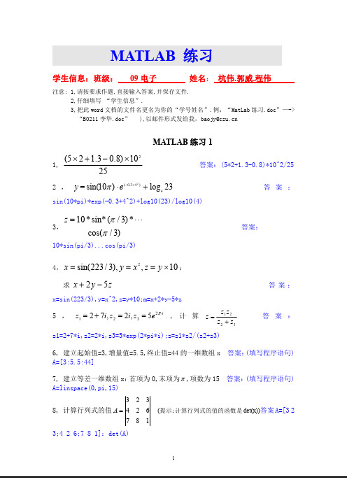
3,
z 10 * sin* ( / 3) * cos( / 3)
答案:
10*sin(pi/3)...cos(pi/3) 4, x 求
sin( 223 / 3), y x 2 , z y 10 ; x 2 y 5z
z1 2 7i, z 2 2i, z 3 5e 2 i , 计 算 z
f ( x ) e sin
3
x
的数值积分 s
f ( x )dx ,并请采用符号计算尝试复算。
fun=inline('exp((sin(x)).^3)');y1=quad(fun,0,pi); 3.绘 制 出 正 态 分 布 N(-1,1) 的 概 率 密 度 函 数 和 分 布 函 数 曲 线 x=(-5:pi/100:5);y=normpdf(x,0,1),plot(x,y)
x=1,f1=(x^3-2*x^2+x-6.3)/(x^2+0.05*x-3.14), x=2,f2=(x^3-2*x^2+x-6.3)/(x^2+0.05*x-3.14), x=3,f3=(x^3-2*x^2+x-6.3)/(x^2+0.05*x-3.14),f1*f2+f3^2
MATLAB 练习 2
1、要求在闭区间[0,2π ]上产生 50 个等距采样的一维数组。试用两种不同的指令实现。 1:A=linspace[0,2*pi,50]; 2:A=[0:2*pi/49:2*pi] 2.说出 MATLAB 指令 A(3,1,2,:)=1:4 所产生数组的维数、大小和长度;然后对 A 进行降维处 理;最后指出降维后 A 中所有非零元素的“单下标”和“全下标”的位置。 A(3,1,2,:)=1:4,ndims(A),size(A),length(A),A(:), A (6) =1=A (3,1,2,1) ; A (12) =2=A (3,1,2,2) ; A(18)=3=A(3,1,2,3) ;A(24)=4=A(3,1,2,4) 3. 写出使以下这段文字成为字符串的 MATLAB 程序。注意保持这段文字的格式。 In GB usage quotation marks are usually single:’Fire!’. S1=char('In GB usage quotation marks are usually single:’Fire!’.') 4. 请建立下列 4×3 的元胞数组 A,如表所示。 张惠妹 周华健 王杰 孙燕姿 听海 花心 一场游戏一场梦 超快感 1998 1992 1988 2000
《MATLAB及应用》实验指导书“作业”
《MATLAB及应⽤》实验指导书“作业”《MATLAB及应⽤》实验指导书班级:姓名:学号:总评成绩:汽车⼯程系电测与汽车数字应⽤中⼼⽬录实验04051001 MATLAB语⾔基础 (3)实验04051002 MATLAB科学计算及绘图 (12)实验04051001 MATLAB语⾔基础实验⽬的1)熟悉MATLAB的运⾏环境2)掌握MATLAB的矩阵和数组的运算3)掌握MATLAB符号表达式的创建4)熟悉符号⽅程的求解实验内容(任选6题)1.利⽤rand等函数产⽣下列矩阵:产⽣⼀个均匀分布在(-5,5)之间的随机阵(50×2),要求显⽰精度为精确到⼩数点后⼀位(精度控制指令为format)。
format banka=-5; b=5;r = a + (b-a).* rand(50,2)r =3.15 -2.244.06 1.80-3.73 1.554.13 -3.371.32 -3.81-4.02 -0.02-2.22 4.600.47 -1.604.58 0.854.57 0.06 -0.15 1.99 3.00 3.91 -3.58 4.59 -0.78 0.47 4.16 -3.612.92 -3.514.59 -2.42 1.56 3.41 -4.64 -2.463.49 3.144.34 -2.56 2.58 -1.502.43 -3.03-1.08 -2.49 1.55 1.16 -3.29 -0.27 2.06 -1.48 -4.68 3.31 -2.23 0.85 -4.54 0.50 -4.03 4.17 3.23 -2.141.952.57-1.83 2.54 4.50 -1.20 -4.66 0.68 -0.61 -4.24 -1.18 -4.46-0.10 -3.70-0.54 0.691.46 -0.312.09 -4.882.55 -1.632.在⼀个已知的测量矩阵T(100×100)中,删除整⾏数据全为0的⾏,删除整列数据全为0的列(判断某列元素是否为0⽅法:检查T(: , i) .* (T(: , i))是否为0)。
matlab综合大作业(附详细答案)

m a t l a b综合大作业(附详细答案)-标准化文件发布号:(9456-EUATWK-MWUB-WUNN-INNUL-DDQTY-KII《MATLAB语言及应用》期末大作业报告1.数组的创建和访问(20分,每小题2分):1)利用randn函数生成均值为1,方差为4的5*5矩阵A;实验程序:A=1+sqrt(4)*randn(5)实验结果:A =0.1349 3.3818 0.6266 1.2279 1.5888-2.3312 3.3783 2.4516 3.1335 -1.67241.2507 0.9247 -0.1766 1.11862.42861.5754 1.6546 5.3664 0.8087 4.2471-1.2929 1.3493 0.7272 -0.6647 -0.38362)将矩阵A按列拉长得到矩阵B;实验程序:B=A(:)实验结果:B =0.1349-2.33121.25071.5754-1.29293.38183.37830.92471.65461.34930.62662.4516-0.17665.36640.72721.22793.13351.11860.8087-0.66471.5888-1.67242.42864.2471-0.38363)提取矩阵A的第2行、第3行、第2列和第4列元素组成2*2的矩阵C;实验程序:C=[A(2,2),A(2,4);A(3,2),A(3,4)]实验结果:C =3.3783 3.13350.9247 1.11864)寻找矩阵A中大于0的元素;]实验程序:G=A(find(A>0))实验结果:G =0.13491.25071.57543.38183.37830.92471.65461.34930.62662.45165.36640.72721.22793.13351.11860.80871.58882.42864.24715)求矩阵A的转置矩阵D;实验程序:D=A'实验结果:D =0.1349 -2.3312 1.2507 1.5754 -1.29293.3818 3.3783 0.9247 1.6546 1.34930.6266 2.4516 -0.1766 5.3664 0.72721.2279 3.1335 1.1186 0.8087 -0.66471.5888 -1.67242.4286 4.2471 -0.38366)对矩阵A进行上下对称交换后进行左右对称交换得到矩阵E;实验程序:E=flipud(fliplr(A))实验结果:E =-0.3836 -0.6647 0.7272 1.3493 -1.29294.2471 0.80875.3664 1.6546 1.57542.4286 1.1186 -0.1766 0.9247 1.2507-1.6724 3.1335 2.4516 3.3783 -2.33121.5888 1.2279 0.6266 3.3818 0.13497)删除矩阵A的第2列和第4列得到矩阵F;实验程序:F=A;F(:,[2,4])=[]实验结果:F =0.1349 0.6266 1.5888-2.3312 2.4516 -1.67241.2507 -0.17662.42861.5754 5.3664 4.2471-1.2929 0.7272 -0.38368)求矩阵A的特征值和特征向量;实验程序:[Av,Ad]=eig(A)实验结果:特征向量Av =-0.4777 0.1090 + 0.3829i 0.1090 - 0.3829i -0.7900 -0.2579 -0.5651 -0.5944 -0.5944 -0.3439 -0.1272-0.2862 0.2779 + 0.0196i 0.2779 - 0.0196i -0.0612 -0.5682 -0.6087 0.5042 - 0.2283i 0.5042 + 0.2283i 0.0343 0.6786 0.0080 -0.1028 + 0.3059i -0.1028 - 0.3059i 0.5026 0.3660 特征值Ad =6.0481 0 0 0 00 -0.2877 + 3.4850i 0 0 00 0 -0.2877 - 3.4850i 0 00 0 0 0.5915 00 0 0 0 -2.30249)求矩阵A的每一列的和值;实验程序:lieSUM=sum(A)实验结果:lieSUM =-0.6632 10.6888 8.9951 5.6240 6.208710)求矩阵A的每一列的平均值;实验程序:average=mean(A)实验结果:average =-0.1326 2.1378 1.7990 1.1248 1.24172.符号计算(10分,每小题5分):1)求方程组20,0++=++=关于,y z的解;uy vz w y z w实验程序:S = solve('u*y^2 + v*z+w=0', 'y+z+w=0','y,z');y= S. y, z=S. z实验结果:y =[ -1/2/u*(-2*u*w-v+(4*u*w*v+v^2-4*u*w)^(1/2))-w] [ -1/2/u*(-2*u*w-v-(4*u*w*v+v^2-4*u*w)^(1/2))-w] z =[ 1/2/u*(-2*u*w-v+(4*u*w*v+v^2-4*u*w)^(1/2))] [ 1/2/u*(-2*u*w-v-(4*u*w*v+v^2-4*u*w)^(1/2))]2)利用dsolve 求解偏微分方程,dx dyy x dt dt==-的解; 实验程序:[x,y]=dsolve('Dx=y','Dy=-x')实验结果:x =-C1*cos(t)+C2*sin(t)y = C1*sin(t)+C2*cos(t)3.数据和函数的可视化(20分,每小题5分):1)二维图形绘制:绘制方程2222125x y a a +=-表示的一组椭圆,其中0.5:0.5:4.5a =;实验程序:t=0:0.01*pi:2*pi; for a=0.5:0.5:4.5; x=a*cos(t); y=sqrt(25-a^2)*sin(t); plot(x,y) hold on end实验结果:2) 利用plotyy 指令在同一张图上绘制sin y x =和10x y =在[0,4]x ∈上的曲线;实验程序:x=0:0.1:4; y1=sin(x); y2=10.^x;[ax,h1,h2]=plotyy(x,y1,x,y2); set(h1,'LineStyle','.','color','r'); set(h2,'LineStyle','-','color','g'); legend([h1,h2],{'y=sinx';'y=10^x'});实验结果:3)用曲面图表示函数22z x y =+;实验程序:x=-3:0.1:3; y=-3:0.1:3; [X,Y]=meshgrid(x,y); Z=X.^2+Y.^2; surf(X,Y,Z)实验结果:4)用stem 函数绘制对函数cos 4y t π=的采样序列;实验程序:t=-8:0.1:8;y=cos(pi.*t/4); stem(y)实验结果:4. 设采样频率为Fs = 1000 Hz ,已知原始信号为)150π2sin(2)80π2sin(t t x ⨯+⨯=,由于某一原因,原始信号被白噪声污染,实际获得的信号为))((ˆt size randn x x+=,要求设计出一个FIR 滤波器恢复出原始信号。
DSP Matlab作业(第5~10章)
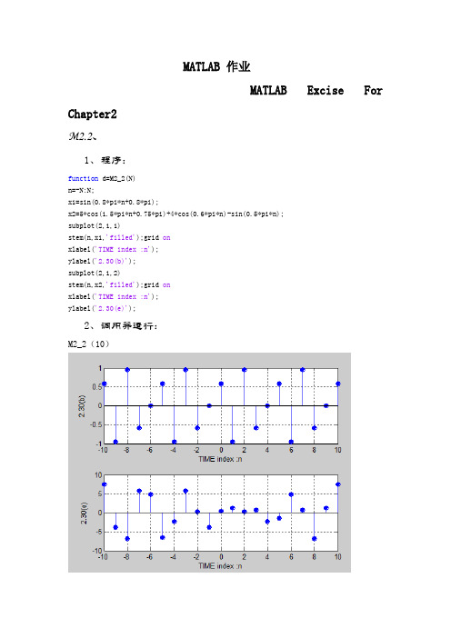
MATLAB 作业MATLAB Excise For Chapter2M2.2、1、程序:function d=M2_2(N)n=-N:N;x1=sin(0.8*pi*n+0.8*pi);x2=5*cos(1.5*pi*n+0.75*pi)+4*cos(0.6*pi*n)-sin(0.5*pi*n);subplot(2,1,1)stem(n,x1,'filled');grid onxlabel('TIME index :n');ylabel('2.30(b)');subplot(2,1,2)stem(n,x2,'filled');grid onxlabel('TIME index :n');ylabel('2.30(e)');2、调用并运行:M2_2(10)M2.3、1、程序:function s=M2_3(A,omega,fai,N)n=0:N;x=A*sin(omega*n+fai);stem(n,x,'fill');grid onaxis([0,N,-2,2]);xlabel('Time index n');ylabel('Amplitude');2、调用并运行(a)、M2_3(1.5,0,pi/2,40)、M2_3(1.5,0.1*pi,pi/2,40)、M2_3(1.5,0.2*pi,pi/2,40)、M2_3(1.5,0.8*pi,pi/2,40)、M2_3(1.5,0.9*pi,pi/2,40)、M2_3(1.5,pi,pi/2,40)、M2_3(1.5,1.1*pi,pi/2,40)、M2_3(1.5,1.2*pi,pi/2,40)(b)、(1)omega=0.6*pi周期T=10;理论上:T=10 (2)omega=0.28*pi周期T=50;;理论上:T=50;(3)omega=0.45*pi周期T=40;理论上:T=40;(4)omega=0.55*pi周期T=40;理论上:T=40;(4)omega=0.65*pi周期T=40;理论上:T=40;M2.9、MATLAB Excise For Chapter3M3.3、调用程序program 3-1运行M3_3Number of frequency points = [1000]Numerator coefficients = 0.2418*[1 0.139 -0.3519 0.139 1] Denominator coefficients = [1 0.2386 0.8258 0.1393 0.4153]The plot of the program are shown in below:运行M3_3Number of frequency points = [1000]Numerator coefficients = 0.1397*[1 -0.0911 0.0911 -1] Denominator coefficients = [1 1.1454 0.7275 0.1205]The plot of the program are shown in below:M3.7、h=input('Type in the target sequence= ');%输入要计算群延时的序列N=input('Type in the group delay frequency point=');%输入要计算的群延时点n=0:(length(h)-1);H=fft(h,N);K=fft(n.*h,N);tao=real(K./H)运行M3-7M3_7Type in the target sequence= [1 1 2 0 0 6 3]Type in the group delay frequency point=8tao =4.0769 7.7221 4.6923 4.0556 9.0000 4.05564.6923 7.7221MATLAB Excise For Chapter5 M5.11、程序function d=M5_1(N)k1=-N:N;x1=ones(1,2*N+1);omega=0:pi/500:2*pi;X1=freqz(x1,1,omega);X1dft=fft(x1);n1=0:1:2*N;figure(1),plot(omega/pi,abs(X1),2*n1/(2*N+1),abs(X1dft),'ro') xlabel('\omega/\pi'),ylabel('Amplitude');k2=0:N;x2=ones(1,N+1);X2=freqz(x2,1,omega);X2dft=fft(x2);n2=0:1:N;figure(2),plot(omega/pi,abs(X2),2*n2/(N+1),abs(X2dft),'ro') xlabel('\omega/\pi'),ylabel('Amplitude');k3=k1;x3=1-(abs(k3)/N);X3=freqz(x3,1,omega);X3dft=fft(x3);n3=n1;figure(3),plot(omega/pi,abs(X3),2*n3/(2*N+1),abs(X3dft),'ro') xlabel('\omega/\pi'),ylabel('Amplitude');x4=N+1-abs(k3);X4=freqz(x4,1,omega);X4dft=fft(x4);figure(4),plot(omega/pi,abs(X4),2*n3/(2*N+1),abs(X4dft),'ro') xlabel('\omega/\pi'),ylabel('Amplitude');x5=cos(pi*k3/(2*N));X5=freqz(x5,1,omega);X5dft=fft(x5);figure(5),plot(omega/pi,abs(X5),2*n3/(2*N+1),abs(X5dft),'ro') xlabel('\omega/\pi'),ylabel('Amplitude');实现了problem3.19中5个序列的求DTFT和DFT2、调用程序运行结果M5_1(8)The red circles denote the DFT samples.当N=8时序列y1的DTFT和DFT采样当N=8时序列y2的DTFT和DFT采样当N=8时序列y3的DTFT和DFT采样当N=8时序列y4的DTFT和DFT采样当N=8时序列y5的DTFT和DFT采样M5.21、程序x=input('the sequence one to convolution;');y=input('the sequence two to convolution;');X=fft(x);Y=fft(y);S=X.*Y;s=ifft(S)2、调用程序M5_2the sequence one to convolution;[5,-2,2,0,4,3]the sequence two to convolution;[3,1,-2,2,4,4]s =10.0000 9.0000 16.0000 44.0000 36.0000 29.0000 M5_2M5_2the sequence one to convolution;[2-j,-1-j*3,4-j*3,1+j*2,3+j*2] the sequence two to convolution;[-3,2+j*4,-1+j*4,4+j*2,-3+j]s =11.0000 +25.0000i -9.0000 +48.0000i 3.0000 +17.0000i 29.0000 + 0.0000i -10.0000 +12.0000iProgram for (c)N=4;n=0:1:N;x=cos(pi*n/2);y=3.^n;X=fft(x);Y=fft(y);S=X.*Y;s=ifft(S)s =-23.0000 -69.0000 35.0000 105.0000 73.0000M5.81、程序X=[11 8-j*2 1-j*12 6+j*3 -3+j*2 2+j 15];k=8:12;XR(k)=conj(X(mod(-k+2,12)));XC=[X XR(k)];x=ifft(XC);n=0:1:11;x1=exp(i*2*pi*n/3);y=x1.*x;output=[x(1) x(7) sum(x) sum(y)];disp(output)disp(sum(x.*x))2、调用程序M5_84.5000 -0.8333 11.0000 -3.0000 - 2.0000i 74.8333MATLAB Excise For Chapter6M6.1(a)、The output of program6_1 by input the coefficient of problem (a)Numerator factors1.00000000000000 -2.10000000000000 5.000000000000001.00000000000000 -0.40000000000000 0.90000000000000Denominator factors1.000000000000002.00000000000000 4.999999999999991.00000000000000 -0.20000000000000 0.40000000000001Gain constant0.50000000000000Then ,The pole-zero plot of is given below:There are 3 ROCs associated with :R1,|z|<;R2,<|z|<; R3,|z|>The inverse –transform corresponding to the ROC is a left-sided sequence, the inverse–transform corresponding to the ROC is a two-sided sequence, and the inverse –transform corresponding to the ROC is a right-sided sequence.(b)、The output of program6_1 by input the coefficient of problem (b)Numerator factors1.00000000000000 1.20000000000000 3.999999999999991.00000000000000 -0.50000000000000 0.90000000000001Denominator factors1.000000000000002.10000000000000 4.000000000000011.00000000000000 0.60000000000003 01.00000000000000 0.39999999999997 0Gain constant1Then ,The pole-zero plot of is given below:There are 4 ROCs associated with :R1,|z|<R2,<|z|<; R3,<|z|<; R4,|z|>The inverse –transform corresponding to the ROC is a left-sided sequence, the inverse–transform corresponding to the ROC is a two-sided sequence, and the inverse –transform corresponding to the ROC is a right-sided sequence.M6.3The output of programme6_4 by type in:(a)M6_3Type in the residues = [-0.8,-7/6]Type in the poles = [-0.2,-1/6]Type in the constants = 3The output is as following:Numerator polynomial coefficients1.0333 0.7333 0.1000Denominator polynomial coefficients1.0000 0.3667 0.0333Hence(b)Rewrite X2(z)asM6_3Type in the residues = [3,-0.7+j*0.6454972243679,-0.7-j*0.6454972243679] Type in the poles = [-0.4,j*0.774596669,-j*0.774596669]Type in the constants = -2.5The output is as following:Numerator polynomial coefficients-0.9000 -2.5600 -0.1000 -0.6000Denominator polynomial coefficients1.0000 0.4000 0.6000 0.2400Hence,(c)M6_3Type in the residues = [5,1.5,-0.25]Type in the poles = [-0.64,-0.5,-0.5]Type in the constants = 0The output is as following:Numerator polynomial coefficients6.2500 6.5500 1.7300 0Denominator polynomial coefficients1.0000 1.6400 0.8900 0.1600Hence,(d)Rewrite X4(z)asM6_3Type in the residues = [-0.75,-0.375+j*0.2905,-0.375-j*0.2905] Type in the poles = [0.5,-j*0.4303,j*0.4303]Type in the constants = -5The output is as following:Numerator polynomial coefficients-4.5000 -6.8750 -3.6375 -0.8438Denominator polynomial coefficients1.0000 1.5000 0.7875 0.1688MATLAB Excise For Chapter7M7.31、程序k = input('Number of frequency points = ');num = input('Numerator coefficients = ');den = input('Denominator coefficients = ');w = 0:pi/(k-1):pi;h = freqz(num, den, w);plot (w,20*log10(abs(h)));gridxlabel('Normalized frequency'); ylabel('Gain, dB');2、调用M7_3运行结果如下M7_3Number of frequency points = 1000Numerator coefficients = [0,1,-2,1]Denominator coefficients = [1,-1.28,0.61+0.4*0.88,-(0.4*0.61)]From the gain response of the transfer function we can get that when the frequency become high and stable then we can conclude that this has a high pass responseM7.51、程序k = input('Number of frequency points = ');num = input('Numerator coefficients = ');den = input('Denominator coefficients = ');w = 0:pi/(k-1):pi;h = freqz(num, den, w);figure(1),plot(w/pi,abs(h));grid ontitle('Magnitude Spectrum')xlabel('\omega/\pi'); ylabel('Magnitude')figure(2),plot(w/pi,angle(h));grid ontitle('Phase Spectrum')xlabel('\omega/\pi'); ylabel('Phase, radians')2、调用M7_5运行结果如下M7_5Number of frequency points = 1000Numerator coefficients = 0.2031*[1,-(1+0.2743),1+0.2743,-1]Denominator coefficients =[1,0.487+0.1532,0.8351+0.83+0.1532*0.487+0.84,0.1532*0.84+0.487*0.8352,0.84*0.8351]Fro m the magnitude response plot given above it can be seen that represents a highpass filter. The difference equation representation of is given byy[n]+0.7074y[n-1]+0.7976y[n-2]+0.2004y[n-3]=0.2031x[n]-0.2588x[n-1]+0.2588x[n-2]-0.2031x[n-3]MATLAB Excise For Chapter9M9.21、程序Fp = input('Passband edge frequency in Hz = ');Fs = input('Stopband edge frequency in Hz = ');FT = input('Sampling frequency in Hz = ');Rp = input('Passband ripple in dB = ');Rs = input('Stopband minimum attenuation in dB = ');Wp = 2*Fp/FTWs = 2*Fs/FT[N, Wn] = buttord(Wp, Ws, Rp, Rs)[b, a] = butter(N, Wn);disp('Numerator polynomial');disp(b)disp('Denominator polynomial');disp(a)[h, w] = freqz(b, a, 512);figure(1),plot(w/pi, 20*log10(abs(h))); grid axis([0 1 -60 5]);xlabel('\omega/\pi'); ylabel('Magnitude, dB'); figure(2),plot(w/pi, unwrap(angle(h))); grid axis([0 1 -8 1]);xlabel('\omega/\pi'); ylabel('Phase, radians');2、调用M9_2运行结果如下M9_2Passband edge frequency in Hz = 10000Stopband edge frequency in Hz = 30000Sampling frequency in Hz = 100000Passband ripple in dB = 0.4Stopband minimum attenuation in dB = 50Wp =0.2000Ws =0.6000N =5Wn =0.2613Numerator polynomial0.0039 0.0197 0.0394 0.0394 0.0197 0.0039Denominator polynomial1.0000 -2.3611 2.6131 -1.5486 0.4864-0.0636M9.111、(a)TF=9kHZ,1pF=1.2kHZ,2pF=2.2kHZ,1sF=650HZ,2sF=3kHZ pα=0.8dB,sα=31dBThenTpp FF112πω==0.8378,Tpp FF222πω==1.536,Tss FF112πω==0.4538,Tss FF222πω==2.094According to bilinear transformation method :)2tan(11ppω=ΩΛ=0.445,)2tan(22ppω=ΩΛ=0.996,)2tan(11ssω=ΩΛ=0.231,)2tan(22s s ω=ΩΛ=1.731. ωB =2p ΛΩ—1p ΛΩ=0.521,s Ω=3.13程序[N, Wn] = cheb1ord(1, 3.13, 0.8, 31, 's');[B, A] = cheby1(N, 0.8, Wn, 's');[BT, AT] = lp2bp(B, A, sqrt(0.43), 0.521);[num, den] = bilinear(BT, AT, 0.5);[h, omega] = freqz(num, den, 256);plot(omega/pi, 20*log10(abs(h)));grid;xlabel('\omega/\pi'); ylabel('Gain,in dB');title('Chebyshev I Bandpass Filter');axis([0 1 -60 5]);2、调用M9_11运行结果如下MATLAB Excise For Chapter10M10.11、程序M1= input('M1= ');M2= input('M2= ');n1=-M1:0.5:M1;n2=-M2:0.5:M2;num1=-0.4*sinc(0.4*n1);num2=-0.4*sinc(0.4*n2);num1(M1+1)=0.6;num2(M2+1)=0.6;w1= 0:pi/(4*M1):pi;w2= 0:pi/(4*M2):pi;h1= freqz(num1, 1, w1);h2= freqz(num2, 1, w2);plot(w1/pi,abs(h1),w2/pi,abs(h2));grid ontitle('Magnitude Spectrum')xlabel('\omega/\pi'); ylabel('Magnitude')2、调用程序运行结果M10.51、程序N = 36;fc = 0.2*pi;M = N/2;n = -M:1:M;t = fc*n;lp = fc*sinc(t);b = 2*[lp(1:M) (lp(M+1) - 0.5) lp((M+2):N+1)]; bw = b.*hamming(N+1)';[h2, w] = freqz(bw, 1, 512);plot(w/pi, abs(h2));axis([0 1 0 1.2]);xlabel('\omega/\pi');ylabel('Magnitude');title(['\omega_c = ', num2str(fc), ', N = ', num2str(N)]);grid on 2、运行结果M10.81、程序wp = 4*(2*pi)/18;ws = 6*(2*pi)/18;wc = (wp + ws)/2;dw = ws - wp;% HammingM = ceil(3.32*pi/dw);N = 2*M+1;n = -M:M;num = (6/18)*sinc(6*n/18);wh = hamming(N)';b = num.*wh;figure(1);k=0:2*M;stem(k,b);title('Impulse Response Coefficients');xlabel('Time index n'); ylabel('Amplitude');figure(2);[h, w] = freqz(b,1,512);plot(w/pi, 20*log10(abs(h))); grid;xlabel('\omega/\pi'); ylabel('Gain, in dB');title('Lowpass filter designed using Hamming window');axis([0 1 -80 10]);% HannM = ceil(3.11*pi/dw);N = 2*M+1;n = -M:M;num = (6/18)*sinc(6*n/18);wh = hann(N)';b = num.*wh;figure(3);k=0:2*M;stem(k,b);title('Impulse Response Coefficients');xlabel('Time index n'); ylabel('Amplitude');figure(4);[h, w] = freqz(b,1,512);plot(w/pi, 20*log10(abs(h)));grid;xlabel('\omega/\pi');ylabel('Gain, in dB');title('Lowpass filter designed using Hann window'); axis([0 1 -80 10]);% BlackmanM = ceil(5.56*pi/dw);N = 2*M+1;n = -M:M;num = (6/18)*sinc(6*n/18);wh = blackman(N)';b = num.*wh;figure(5);k=0:2*M;stem(k,b);title('Impulse Response Coefficients');xlabel('Time index n'); ylabel('Amplitude');figure(6);[h, w] = freqz(b,1,512);plot(w/pi, 20*log10(abs(h)));grid;xlabel('\omega/\pi');ylabel('Gain, in dB');title('Lowpass filter designed using Blackman window'); axis([0 1 -80 10]);2、运行结果M10.91、程序beta = 3.631;N = 44;n = -N/2:N/2;num = (6/18)*sinc(6*n/18);wh = kaiser(N+1,beta)';b = num.*wh;figure(1);stem(b);title('Impulse Response Coefficients');xlabel('Time index n');ylabel('Amplitude')figure(2);[h, w] = freqz(b,1,512);plot(w/pi, 20*log10(abs(h)));grid;xlabel('\omega/\pi');ylabel('Gain, in dB');title('Lowpass filter designed using Kaiser window'); axis([0 1 -80 10]);2、运行结果。
- 1、下载文档前请自行甄别文档内容的完整性,平台不提供额外的编辑、内容补充、找答案等附加服务。
- 2、"仅部分预览"的文档,不可在线预览部分如存在完整性等问题,可反馈申请退款(可完整预览的文档不适用该条件!)。
- 3、如文档侵犯您的权益,请联系客服反馈,我们会尽快为您处理(人工客服工作时间:9:00-18:30)。
MATLAB
作业5
1、 试求解下面微分方程的通解以及满足(0)1,()2,(0)0x x y π===条件下的解析解。
66()5()4()3()sin(4)2()()4()6()cos(4)
t t x t x t x t y t e t y t y t x t x t e t --⎧+++=⎨+++=⎩ 解:
>> syms t x y;
>>[x,y]=dsolve('D2x+5*Dx+4*x+3*y=exp(-6*t)*sin(4*t)',
'2*Dy+y+4*Dx+6*x=exp(-6*t)*cos(4*t)','x(0)=1','x(pi)=2','y(0)=0');vpa(x,20)
ans =
.24816266536011758942e-1*exp(-6.*t)*cos(4.*t)-.16682998530132288094e-1*exp(-6.*t)*sin(4.*t)+.85861668591377882749e-1*exp(t)-.57658489325155296910e-1*exp(-5.1374586088176874243*t)+.94698055419776565523*exp(-1.3625413911823125757*t)
>>vpa(y,20)
ans =
-.10607545320921117099*exp(-6.*t)*cos(4.*t)+.68348848603625673689e-1*exp(-6.*t)*sin(4.*t)-.28620556197125960916*exp(t)+.90450561852315609427e-1*exp(-5.1374586088176874243*t)+.30183045332815517077*exp(-1.3625413911823125757*t)
2、 Lotka-Volterra 扑食模型方程为()4()2()()()()()3()
x t x t x t y t y t x t y t y t =-⎧⎨=-⎩,且初值为(0)2,(0)3x y ==,
试求解该微分方程,并绘制相应的曲线。
解:
>>syms x y t;
>> f=inline('[4*x(1)-2*x(1)*x(2); x(1)*x(2)-3*x(2)]','t','x');
>> [t,x]=ode45(f,[0,10],[2;3]);plot(t,x)
3、 是给出求解下面微分方程的MA TLAB 命令,
(3)22,(0)2,(0)(0)0ty y tyy t yy e y y y -++====
并绘制出()y t 曲线。
试问该方程存在解析解吗?选择四阶定步长Runge-Kutta 算法求解该方程时,步长选择多少可以得出较好的精度,MATLAB 语言给出的现成函数在速度、精度上进行比较。
解:
>> f=inline('[x(2); x(3); -t^2*x(1)*x(2)-t^2*x(2)*x(1)^2+exp(-t*x(1))]','t','x');
[t,x]=ode45(f,[0,10],[2;0;0]); >> plot(t,x)
4、 试用解析解和数值解的方法求解下面的微分方程组
5()2()3(),(0)1,(0)2()2()3()4()4()sin ,(0)3,(0)4t x t x t x t e x x y t x t y t x t y t t y y -⎧=--+==⎨=----==⎩
解:
解析解:
>> syms t x y;
[x,y]=dsolve('D2x=-2*x-3*Dx+exp(-5*t)','D2y=2*x-3*y-4*Dx-4*Dy-sin(t)','x(0)=1','Dx(0)=2','y(0)=3','Dy(0)=4')
x =
1/12*exp(-5*t)-10/3*exp(-2*t)+17/4*exp(-t)
y =
-265/16*exp(-t)-71/5*exp(-3*t)+11/48*exp(-5*t)+100/3*exp(-2*t)+51/4*exp(-t)*t+1/5*cos(t)-1/10*sin(t)
数值解:
>> f=inline('[x(2); -2*x(1)-3*x(2)+exp(-5*t); x(4); 2*x(1)-3*x(3)-4*x(2)-4*x(4)-sin(t)]','t','x');
[t1,x1]=ode45(f,[0,10],[1;2;3;4]);
ezplot(x,[0,10]), line(t1,x1(:,1)) figure; ezplot(y,[0,10]), line(t1,x1(:,3))
5、 下面的方程在传统微分方程教程中经常被认为是刚性微分方程。
使用常规微分方程解法和刚性微分方程解法分别求解这个微分方程的数值解,并求出解析解,用状态变量曲线比较数值求解的精度。
11212122119245cos sin ,(0)331224519cos sin ,(0)33
y y y t t y y y y t t y ⎧=++-=⎪⎪⎨⎪=---+=⎪⎩ 解:
>> syms t y1 y2;
>>
[y1,y2]=dsolve('Dy1=9*y1+24*y2+5*cos(t)-1/3*sin(t)','Dy2=-24*y1-51*y2-9*cos(t)+1/3*sin(t)','y1(0)=1/3','y2(0)=2/3')
y1 =2/(3*exp(3*t)) - 2/(3*exp(39*t)) + cos(t)/3
y2 =4/(3*exp(39*t)) - 1/(3*exp(3*t)) - cos(t)/3
6、试用数值方法求解偏微分方程
22
22
0,00,0
1,0
0,0
x y y x
u u
x y
u u
x y
=>=≥
⎧∂∂
+=
⎪∂∂
⎪⎪
==
⎨
⎪
>>
⎪
⎪⎩
,并绘制出u函数曲面。