数理经济学lecture12
数理经济学教学大纲期末复习
数理经济学教学大纲期末复习《数理经济学》教学大纲一、课程基本信息课程代码 03323990 课程类别专业发展课程—选修课中文名称数理经济学英文名称Mathematical Economics适用专业经济学专业开课单位经济系总学时 54 (理论:48 其他:6 ) 学分 3先修课程经济数学基础,西方经济学后续课程计量经济学,数学建模,毕业设计二、课程性质、地位和任务数理经济学是经济学专业的选修课,强调运用数学方法,主要是微积分、线性代数、数理统计方法来解决经济学中的一些原理问题。
从性质上说,数理经济学是利用数学方法对经济问题进行分析演绎,因而是进行经济理论研究必备的重要工具。
因此,本课程既不能等同于纯粹的中高级西方经济学,也不能等同于一般的经济数学。
本课程通过对数学方法与经济模型结合,主要目的在使学生熟习如何应用数学模型来表述经济学,旨在提高经济学分析中的数理思维能力,培养学生运用数学工具进行经济学研究的能力,为将来的深入学习和研究打下必要的方法论基础。
三、课程基本要求本课程通过讲授、练习和阅读文献等形式,使学生掌握主要的数理经济学研究方法,了解其主要工具和概念,掌握微分、矩阵、最优化的基本原理和方法,并能运用所学数理工具分析一些理论与现实经济问题,从而对现实经济系统进行预测与决策。
四、课程内容及学时分配序号内容学时第一章导论 3第二章单变量微分法及其经济学应用 6第三章单变量最优化问题 12第四章线性模型与矩阵代数 9第五章多变量微分法及其经济学应用 12第六章多变量最优化问题 12合计 54第一章导论【教学内容】数理经济学的概念、数理经济学的起源和发展、数理经济学的研究对象、研究方法。
【教学基本要求】通过本章的学习,使学生了解数理经济学的产生和发展、数理经济学的研究方法,理解经济模型的构成及其作用。
【教学安排】课堂讲授3学时【重难点】数理经济学的研究方法、经济模型第一节数理经济学的产生和发展第二节数理经济学的研究方法第三节经济模型第二章单变量微分法及其经济学应用【教学内容】连续函数,导数和微分,经济学中的“边际”概念,反函数,经济学中的增长率【教学基本要求】复习单变量微分法基本数学原理;掌握经济学中各种函数连续性及其可微性;深刻认识边际、弹性与增长率的概念,理解它们与微分之间的关系。
数理经济学课件.docx
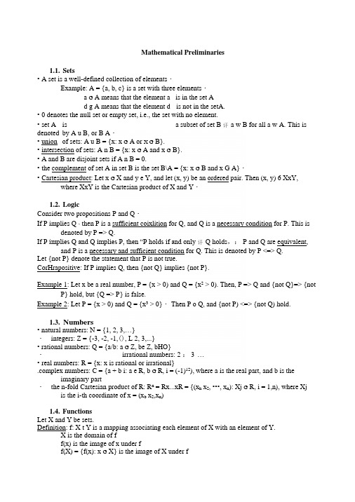
Mathematical Preliminaries1.1.Sets•A set is a well-defined collection of elements・Example: A = {a, b, c} is a set with three elements・a G A means that the element a is in the set Ad g A means that the element d is not in the setA.•0 denotes the null set or empty set, i.e., the set with no element.•set A is a subset of set B 讦a w B for all a w A. This is denoted by A u B, or B A・•union of sets: A u B = {x: x G A or X G B}.•intersection of sets: A n B = {x: x G A and x G B}.•A and B are disjoint sets if A n B = 0.•the complement of set A in set B is the set B\A = {x: x G B and x G A}・•Cartesian product: Let x G X and y e Y, and let (x, y) be an ordered pair. Then (x, y) 6 XxY, where XxY is the Cartesian product of X and Y・1.2.LogicConsider two propositions P and Q・If P implies Q、then P is a sufficient coixlition for Q, and Q is a necessary condition for P. This is denoted by P => Q.If P implies Q and Q implies P, then “P holds if and only 讦Q holds,: P and Q are equivalent, and P is a necessary and sufficient condition for Q. This is denoted by P <=> Q.Let {not P} denote the statement that P is not true.CorHrapositive: If P implies Q, then {not Q} implies {not P}.Example 1: Let x be a real number, P = {x > 0) and Q = {x2 > 0). Then, P => Q and {not Q}=> {not P} hold, but {Q => P} is false.Example 2: Let P = {x > 0) and Q = {x3 > 0}・ Then P o Q, and {not P) <=> {not Q) hold.1.3.Numbers•natural numbers: N = {1, 2, 3,…}・integers: Z = {-3, -2, -1,(), L 2, 3,...}•rational numbers: Q = {a/b: a G Z, be Z, bHO}・irrational numbers: 2 : 3 …•real numbers: R = {x: x is rational or irrational}.complex numbers: C = {a + b i: a e R, b G R, i = (-1)12), where a is the real part, and b is the imaginary part・the n-fold Cartesian product of R: R n = Rx...xR = {(x h x2, •••, x n): Xj G R, i = 1,n), where Xj is the i-th coordinate of x = (x b x2,x n)1.4.FunctionsLet X and Y be sets.Definition: f: X t Y is a mapping associating each element of X with an element of Y.X is the domain of ff(x) is the image of x under ff(X) = {f(x): x G X} is the image of X under f•a function: if only one point in Y is associated with each point in X・ a coirespondence: if more than one point in Y can be associated with each point in X •inverse function: x = f *(y) if and only if y = f(x).a function f: X T Y is onto 讦f(X) = Y.It means that the equation f(x) = y has at least one solution for each y.•if f(x) and f ly) are both single・valued, then f is on—to-one.It means that the equation f(x) = y has at most one solution for each y.•composite function: h = g(f(x)) = g • f is the composition of f with g satisfying f: A t B u C, g:C t D, g • f: A t D.L5e BoundsLet S c R.•S is bounded from above (from below)讦there exists a G R (b G R) such that x < a (x > b) for all x G S. Then, a is an upper bound of S, and b is a lower bound of S・•The least upper bound (lub) or suDremum (sup) of S is the upperbound of S such that there does not exist a smaller upper bound. It is denoted by sup(S).•The supremum of S is called a maximum (max) of S if sup(S) G S. It is denoted by max(S). •The greatest lower bound (gib) or infimum (inf) of S is the lower bound of S such that there does not exist a larger lower bound. 1( is denoted by inf(S).•The infimum of S is called a minimum (min) of S if inf(S) e S. It is denoted by min(S).• Property:If S c R and S has an upperbound, then S has a supremum.If S u R and S has a lowerbound, then S has an infimum.16 Vector SpaceConsider a set V.LI- associative law: x + (y + z) = (x + y) + z, for all x, y, z, w VL2- identity: there exists O G V such that x + 0 = x for all x G VL3- inverse: there exists (-x) e V such that x + (-x) = 0 for all x e VL4- commutative law: x + y = y + x for all x, y G VL5- associative law: a・([3・x) = (a-p) x for all a, p e R, and for all x G VL6- identity: there exists 1 G V such that l x = x for all x e VL7- distributive law: a・(x + y) = a x + a y for all ae R, and for all x, y w VL8- distributive law: (a + p)-x = a x + p x for all a,卩G R, and for all x G V L9- closure: x e V and y G V implies that (x + y) G V LIO- closure: x G V and ae R implies that (a・x) e V. Definition: A set V is vector space (or linear space) if it satisfies Ll-Ll0. Then x G V is called a vector. Examples: R l\ or C n is each a vector space.1.7. Norms and distancesConsider a function d(x, y) satisfying:M1: d(x, y) = 0 if and only if x = y M2: d(x, y) + d(y, z) > d(z, x) M3: d(x, y) > 0 for all x, y M4: d(x, y) = d(y, x).Definition: For a given set X,讦a function d: XxX —> R satisfies M1-M4, then: X is a metric space, denoted by (X, d)d is a metricd(x, y) is the distance between points x and y.Examples:di(x,y) = [Zi (xj - yi)2!12 = Euclidian distance,denoted by ||x - y||d2(x, y) = maxi 风-y s|d3(x, y) = Zi lx, - y.lNote: Topology consists in studying the properties of sets that are independent of the distance measure chosen.Definition: Let V be a vector space・ A real value function N: V t R is called a norm on V if: N(x) > 0 for all x G V N(x) = 0 if and only if x = 0N(r x) = |r| N(x) for all re R and x e V, andN(x + y) < N(x) + N(y) for all x, y G V.Example: N(x) = d|(x, 0) = [Xi (xj)2]12 = ||x|| is the Euclidian noim of x in R.R n, with Euclidian norm and Euclidian metric, is a normed vector space.Every normed vector space is a metric space with respect to the induced metric defined by d](x, y) = llx - yll.Convex SetsLet X be a vector space (e.g・,X = R n).Definition: A set S c: X is convex if any x, y G S implies that(0x + (1-0) y) e S, for all 0 e R, 0 < 0 < 1.Note: (0 x + (1-0) y) is called a linear combination of x and y.Properties:・Any intersection of convex sets is convex.•Let Si, i = 1,m, be convex sets in vector space X. Then:•(Ejei (Xj Si) = {x: x = Z i=i■•…m oti Xi, XjG Sj, otf R, i = 1,…,Hi} is a convexset.•(SixS2x...xS m) = x i=1■•…m (Si) is a convex set.L9. Compact SetsLet S u R n.Definition: An open ball about x0 e R n with radius r e R, r > 0, is defined as:B r(x0) = {x: x G S, d(x, x0) < r}, where d(x, x0) is the Euclidian distance betweenpoints x and x0.Definition: An open set S u R n is a set S such that, for each x e S, there exists an open ball B r(x) completely contained in S.• The union of open sets is open..A finite intersection of open sets is open.Definition: The inierior of a set S, denoted by int(S), is the union of all open sets contained in S..A set S is open 讦and only 讦S 二int(S).Definition: A set S c R n is closed 讦the set (R n\S) is open.・The intersection of closed sets is closed・.A finite union of closed sets is closed・Definition: The closure of a set S, denoted by cl(S), is the intersection of all closed sets containing S..A set S is closed if and only if S = cl(S).Definition: The boundary of a set S u R" is the set cl(S)ncl(R n/S).Definition: A set S is bounded if there exists an open ball with a finite radius which contains S・Definition: A collection of open sets (S a)a€A in a metric space X is said to be an open cover of a given set S u R n if S u 低入 S a.The open cover (S a)ae A of S is said to admit a finite subcover if there exists a finitesubcollection (SQ^F such that S u S®Definition 1: A set S c R n is compact if and only if it is closed and bounded・Definition 2: A subset S of a metric space X is compact if and only if every open cover of S has a finite subcover.Note: The definition 2 of compactness applies to sets in any metric space, while definition 1 applies only to sets in R n.LIO. SequencesLet (X, d) be a metric space (e.g., X = R n), and let S c X.Definition: A sequence {xj: j = 1,g} in S converges to y if, for any e > 0, there exists a positive integer j" such that j hj,implies d(y, xj) < e.This is denoted by y = limj* {xj, where y is the limit of {Xj}.Note: It does not follow that y = lirOjT® {xj} G S・Definition: A sequenee {Xj: j = 1,…,g} in S is a Cauchy sequence if for any e > 0, there exists a positive integer such that, for any ij > j\ d(x i9 Xj) < £.Definition: If every Cauchy sequence in a metric space is also a convergent sequence, then the* A sequence {xp j = 1,…严} in R" is a Cauchy sequence if and only if it is a convergent sequence, i.e. if and only if there is y G R n such that linij》{Xj} —> y.metric space is said to be complete.By the above definition, this implies that R n is complete (although not all metric spaces are complete)・Definition: Let m(j) be an increasing function: m: {12 3,…} T {1, 2, 3,such that m(k+l) > m(k).Given a sequence {xj: j = 1, 2,…,g}, {m = 1,…,g} is a subsequence of {xj: j =1,2,…,oo}..A set S c R n is closed if and only if every convergent sequenee of points in S converges to a point in S・・ A set S e R n is compact if and only if every sequence in S has a convergent subsequence whoselimit is in S.・ A sequence {xj: j = 1, 2,…,g} in R n converges to y if and only if every subsequence of {xj: j =1,…,g} converges to y.・Every bounded sequence contains a convergent subsequence・Definition: A sequence {xj: j = 1,2,…,oo} is (strictly) increasing if, for all m > n, x m > (>) x n for all n.A sequence {xj: j = 1,2,…,<»} is (strictly) decreasing if, for all m > n, x m < (<) x n forall n・Let X u R, X H 0. If X is bounded from above (below), there exists an increasing (decreasing) sequence in X converging to sup(X) (inf(X)).Definition: Assume that ±oo are allowed as limits of a sequence.The lim sup of the sequence {xj: j = 1,in R is defined as limj^oo {可:j =1,2 •••}, where aj = sup{xj, Xj+b Xj+2. ...}・ It is denoted by linij^oo supk>j x k, or simply by lim SUpjTco Xj・The lim inf of the sequence {Xj: j = 1,in R is defined as limj^ {bj: j = 1,2 …}, where bj = inf{x jt Xj+i, x i+2, ...}. It is denoted by inf k>j x k, or simply by lim infj†Xj・† A sequence xj in R converges to a limit y G R if and only if y = lim supj* Xj = lim in与* Xj.。
数理经济学精要

约束为资本的储蓄方程式:
K = I − δ K
§3 变分法
14
例3.1.2 最优资本存量问题
由此问题的 Euler 方程可推导出:
FK
=
⎛ ⎜
r
⎝
+δ
−
p p
⎞ ⎟ ⎠
p
该方程左边表示资本的边际收益,右边表示资本的
实际成本,它等于用投资品价格衡量的利息和折旧
与因资本价格变动带来的收益(购入后资本价格升
§3 变分法
22
可变端点变分问题的Euler方程
【定理 3.2.3】(可变端点变分问题的 Euler 方程和横 截性条件)
设 f ,ψ 为二阶连续可微函数, x∗,t1*为变分法 问题(CVP-4)的最优解,则 Euler 方程(3.1.2)成立,且 满足下述边界条件
⎡⎣ f (t, x∗, x∗ ) + (ψ − x∗ ) fx (t, x∗, x∗ )⎤⎦t=t1* = 0 (3.1.7)
(3.1.4)
L(t, x(t), x(t)) = f (t, x(t), x(t)) + μT g(t, x(t), x(t))。
§3 变分法
17
例3.2.1:等周问题
如下图,考虑连接两点 A、B 的长度为一定的, 与线段 AB 围成的面积最大的曲线。
y
A
B
x0 图 3.2.1 等周问题 x1 x
厦门大学经济系 邵宜航
数理经济学精要
——经济学中的最优化数学分析
变分法原理与应用 (讲义要点)
第三章 变分法
§3.1 最简变分问题 §3.2 条件变分和可 动边界变分
3.1.1. 最简泛函的第一 变分与第二变分
《数理经济学》课件

数学符号在数理经济学中具有特定的意义,它们代表了经济变量、参数和函数等。理解这些符号的意义 是理解数理经济学理论的关键。
数学模型与方程
01
模型构建
数理经济学家使用数学模型来描述经济系统。这些模型通常由一组方程
式构成,用来表示不同经济变量之间的关系。
02
方程类型
在数理经济学中,常见的方程类型包括线性方程、非线性方程、微分方
数理经济学的发展历程
总结词
数理经济学的发展历程可以追溯到19世纪,其发展经 历了多个阶段,包括古典数理经济学、新古典数理经 济学和现代数理经济学等。
详细描述
数理经济学的发展历程可以追溯到19世纪,当时一些 经济学家开始尝试运用数学方法来描述和预测经济现 象。古典数理经济学阶段主要关注生产、分配和交换 等经济活动的均衡问题。新古典数理经济学阶段则强 调个体行为和市场均衡的研究,并引入了边际分析和 效用函数等概念。现代数理经济学则更加注重数学模 型的复杂性和精确性,并广泛应用于宏观和微观经济 学等领域。
在数理经济学中,证明方法多种多样 ,包括直接证明、反证法、归纳法和 演绎法等。这些方法用于证明经济定 理和推导经济关系,确保经济理论的 严谨性和准确性。
在数理经济学中,必须遵循一定的推 理原则,如公理化原则、一致性原则 和完备性原则等。这些原则确保了经 济理论的逻辑严密性和科学性。
03
数理经济学的应用
宏观经济学中的应用
经济增长与经济发展
数理经济学在研究经济增长、经济发展等方面发挥了重要作用,通 过建立数学模型来解释国家或地区的经济增长和发展趋势。
财政政策与货币政策
利用数理经济学方法分析财政政策和货币政策的效果,为政府制定 经济政策提供科学依据。
厦大《数理经济学》参考文献

《数理经济学》课程参考文献(著作、教材类)注:以下所列文献难度各异,如需阅读建议请联系任课老师。
[1]Avriel, M., Nonlinear Programming: Analysis and Methods, EnglewoodCliffs: Prentice-Hall, 1976.[2]Barro, R. J. and X. Sala-I-Martin, Economic Growth, New YorK:McGraw-Hill, 1995.[3]Bazaraa, M. S., H. D. Sherali, and C. M. Shetty. Nonlinear Programming:Theory and Algorithms. New York: John Wiley & Sons, 1979.[4]Blanchard, M. and S. Fischer, Lecture on Macroeconomics, Cambridge:MIT Press, 1989.[5]Carlson, D. A. A. B. Haurie, A. Leizarowitz, Infinite Horizon OptimalContral, Berlin: Springer-Verlag, 1991.[6]Dixit, A. K. Optimization in Economic Theory, Oxford: OxfordUniversity Press, 1990.[7]Girsanov, I. V., Lecture on Mathematical Theory of Extremum Problems,Berlin: Springer-Verlag, 1972.[8]Hestenes, M. R., Calculus of Variations and Optimal Control Theory, NewYork: John Wiley & Sons, 1966.[9]Intriligator, M. D. Mathematical Optimization and Economic Theory,Englewood Cliffs: Prentice-Hall, 1971.[10]Ioffe, A. D. and V. M. Tihomirov, Theory of Extremal Problems,Amsterdam: North-Holland, 1979.[11]Jehle, G. A. and P. J. Reny, Advanced Microeconomic Theory, 2nd ed., 上海财经大学出版社,影印本。
数理经济学

2011-4-30
IV.12.2
GuoSipei@CCNUMATH
求稳定值
• 拉格朗日乘数法
其实质是将约束极值问题转化为另一种等价形式, 从而使得自由极值问题的一阶条件仍然可以应用. 问题:给定U=x1x2+2x1,约束条件4x1+2x2=60, 求U的极大值.
先写出拉格朗日函数,它是容纳了约束条件的目标函数的 变形:Z=x1x2+2x1+λ(60-4x1-2x2) 如果约束条件得到满足(上式括号中的部分等于0),则无 论λ(拉格朗日乘数)取何值Z=U,于是,问题转化为加入变 量λ后的,Z的自由极值问题
第四篇 最优化问题
• 第12章 具有约束方程的最优化
约束的影响 求稳定值 二阶条件 拟凹性和拟凸性 效用最大化与消费需求 齐次函数 投入的最小成本组合
2011-4-30
IV.12.1
GuoSipei@CCNUMATH
约束的影响
• 约束
一个约束确立了两个变量在充当选择变量时的关系, 但这种关系与其他类型的将两个变量联系在一起的 关系是不同的. 施加约束的基本目的是对在所讨论的最优化问题中 存在的某些限制因素给出合理的认识 生产配额问题是典型的约束最优化问题 约束的作用在于缩小定义域,从而缩小目标函数的 值域
2011-4-30
IV.12.15
GuoSipei@CCNUMATH
2011-4-30
IV.12.16
GuoSipei@CCNUMATH
• 代数定义
三个相关定理:
2011-4-30
IV.12.17
GuoSipei@CCNUMATH
有用的说明:
两个拟凹函数的和不一定是拟凹函数 检验拟凹性和拟凸性的简便方法:
数理经济学lecture11
function can be written as ln f =
the sum is concave. But f is then a monotonic transformation of a concave function and hence quasi-concave.
3
3.1
Economic Applications I - Consumer Theory
2
Concave Programing
With concave functions, we can conclude from the FOC that we have a global maximum.
Theorem 3 Let U ⊂ Rn be convex and open. Let f : U → R be C 1 and concave. Suppose that g1 , .., gm are convex functions U → R. max f (x) st g (x) ≤ 0. (note that constrained set is convex). ¯ st: Suppose you can find x ¯ ∈ U and λ ∇f (¯ x) =
Lecture XII: Concave Programming
Markus M. Mobius November 5, 2002
1
Second Order Conditions
We ask two further questions: (1)( How can we know if a local extremum is a maximizer or minimizer? This raises the question of second order conditions. (2) How can we ensure that a local maximizer/ minimizer is a global maximizer/ minimizer? • In the unconstrained case, we simply look at the Hessian matrix of the objective function. • In the constrained case, we can only move along the constrained surface. As a result, the SOC only has to be true along the tangent subspace. The tangent subspace is the set of points orthogonal to the vectors ∇gk (¯ x), k = 1, .., m. We say that a matrix A is negative definite on a subspace V of Rn iff v Av ≤ 0 for all v ∈ V.
数理经济学
2011-4-30
I.25
GuoSipei@CCNUMATH
2.4 关系与函数
2011-4-30 I.15 GuoSipei@CCNUMATH
数学方法具有如下优点:
运用的“语言”更为简练、精确 有大量的数学定理可为我所用 迫使我们明确陈述所有假设,作为运用数学定理的 先决条件,这能使我们戒除不自觉地采用不明确假 设的缺点 使我们能够处理n个变量的一般情况
本课程的目的就是将经济学文献中相关的数学 方法汇聚到一处,按逻辑顺序组织,完整地解 释,并阐述其在经济学中的应用
第一篇 导 论
第1章 数理经济学的实质
1.1 数理经济学与非数理经济学 1.2 数理经济学与经济计量学
第2章 经济模型
2.1 2.2 2.3 2.4 2.5 2.6 2.7
2011-4-30
数学模型的构成 实数系 集合 关系与函数 函数的类型 两个或两个以上自变量的函数 一般性水平
I.1 GuoSipei@CCNUMATH
注:当未特别设定时,我们将定义域和值域理解为 仅包括使函数具有经济意义的那些数值.
2011-4-30
I.27
GuoSipei@CCNUMATH
2.5 函数的类型
常值函数
在平面直角坐标系中这样的函数表现为一条水平线 在国民收入模型中,当投资(I)为外生决定的,可以有下 述形式的投资函数:I=1亿美元,或I=I0
数学定理按照“如果-那么”的形式陈述,为导出“那么”,分析者 必须保证每个分析阶段中“如果”与其采纳的假设相一致 超越几何学分析方法是完全有必要的:方程工具打破维数限制,分 析更一般的情况,如无差异曲线的一般图形讨论时,标准假设是消 费者只能得到2种商品,因为要绘出3维或更多维的图形是基本不现 实的
数理经济学
数理经济学
数理经济学是一门研究数量和经济行为的综合学科,它对数学、统计学和经济学的应用相结合。
它的出现开拓了经济学的发展范围,深入剖析经济存在的问题,提供有效的解决解决方案,并实施经济政策。
数理经济学主要通过定量分析及模型去研究社会经济现象和政策,比如微观经济,宏观经济,货币市场,国际经济等等。
数理经济学运用了数学、统计、技术分析和实验方法来建模经济各类问题和政策,推导出有效的经济分析结果以及经济政策可行性分析。
数理经济学还有助于更好地理解复杂的经济系统,比如,金融市场中各类金融资产价格的变化,这些价格变化受多种因素共同影响,既有宏观因素也有微观因素,数理经济学使分析师们能够深入分析相关问题,并利用概率模型来研究当前的经济形势和走势。
总而言之,数理经济学运用了数学、统计、技术分析和经济学的原理,以及实验和模型等,来研究经济现象。
它为经济研究和经济政策制定提供了有效的方法,这极大地推动了经济发展和改善了现实经济环境。
Economics(数理经济学基础)
Syllabus of『Fundamental Methods of Mathematical Economics』(数理经济学基础)Course DetailsSemester: 2005-2006学年,第2学期Lecturer 张明恒PhD., Associate ProfessorOffice: (教学行政大楼) Teachers Official Buildings 512RoomOffice Time: P.M.6:30 – 8:30, TuesdayTelephone: +86 21 6590 2567E-Mail: mingheng@Coordinator:Date: 3/4,Wed;1/2,FridayRoom: 1405Rm, No.1 Teaching Buildings(1405,国定路一教) Website: /~mingheng/MathEcon.htmlStudent Background(i)the pre-session mathematics course(ii)the background mathematical material(iii)the fundamental of EconomicsGeneral AdviceThe key to success in a course like mathematical economics is to work carefully and consistently on the course material as the semester progresses. Falling behind with the course material is a recipe for disaster. Therefore students are strongly urged to attempt to complete the exercise sheets prior to attending the examples class and to read the appropriate chapters in the course text in conjunction with their lecture notes.The learning resources(i)the office hours of the lecturer when he will be available to see students;or make appointment by email or phone to meet the lecturer at anothertime(ii)the textbooks (incl. the materials on the classroom)(iii)the materials on the course web page(iv)the discussion with (the advice from) colleagues and friends on the course AimsThe aims of this course are to(i)Provide an introduction to mathematical methods for economics that willassist students in understanding mathematical research in their field;(ii)Enable students to apply these mathematical methods in their own research.ObjectivesAt the end of the course students should be able to(i) Demonstrate their understanding of the mathematical methods foreconomics;(ii)Understand and study Equilibrium Analysis, Comparative Statics Analysis, Optimization (multivariate), Dynamic Economic, Simultaneous Equations andLinear Programming etc.;(iii)Ready to advanced microeconomics, macroeconomics and econometrics.List of Readings1)Chuang,A.C., Fundamental Methods of Mathematical Economics,McGraw-Hill Publishing Company, 1984, 3rd Ed. (刘学译, 数理经济学的基本方法, 商务印书馆,2003年)(Text Book).2)Silbergerg, E., The Structure of Economics – A Mathematical Analysis,McGraw-Hill Education - Europe, 1990, 2nd ed, paperback.3)Klein,M.W., Mathematical methods for Economics, Addison-Wesley, 1998.4)Dowling,E.,T., Theory and Problems of Introduction to Mathematical Economics, 3nd5)Handbook of Mathematical Economics Vol.1-6,6)International Journal on Mathematical Economics such asi.Journal of Mathematical Economicsii.Journal of Economics Theoryiii.Journal of Economics and Businessiv.Journal of Mathematical Financev.Journal of Econometricsvi.Mathematical Social Sciencesvii.Economics Modellingviii.Economics Lettersix.Economics Theoryx.Game TheoryLecturesChapter 1 Nature of Mathematical Economics/数理经济学的实质Chapter 2 Economic Models/经济模型Chapter 3 Equilibrium Analysis in Economics/静态均衡分析,市场均衡模型,国民收入均衡模型Chapter 4 Linear Models and Matrix Algebra/线性模型与矩阵代数Chapter 5 Linear Models and Matrix Algebra/线性模型与矩阵代数,市场模型,国民收入模型,Leontief投入产出模型Chapter 6 Comparative Statics and the Derivative/比较静态分析,变化率/导数/曲率,极限定理,函数的连续性与可微性Chapter 7 Rules of Differentiation and Comparative Statics,微分法则,偏微分,Jacobi行列式Chapter 8 Comparative Statics of General Function Models,全微分/全导数,隐函数存在定理,一般函数模型的比较静态分析Chapter 9 Optimization (univariate),最优值与级值,导数检验,Maclaurin/Taylor 级数Chapter 10 Exponential and Logarithmic Functions/指数函数与对数函数,自然指数与增长问题,最优时间安排Chapter 11 Optimization (multivariate)/多变量的最优化,最优化条件的微分形式,二次型,目标函数,Hessian矩阵检验,函数的凹/凸性与极值问题,多产品厂商问题,价格歧视,投入决策Chapter 12 Optimization with Equality Constraints/具有约束方程的最优化,Lagrange Multiplier, Bordered Hessian Matrix检验,二阶条件效用最大化与消费需求,齐次函数/生产函数,投入最小成本组合Chapter 13 Economic Dynamics and Integral Calculus/动态经济学与积分学,动态与积分,定积分/不定积分/广义积分,Domar增长模型Chapter 14 First Order Differential Equations/连续时间的一阶微分方程,市场价格的动态过程,恰当微分方程,非线性微分方程Solow增长模型Chapter 15 Higher Order Differential Equations/高阶微分方程,复数,三角函数,复数根,具有价格预期的市场模型、通货膨胀与失业模型Chapter 16 First Order Difference Equations/离散时间的一阶差分方程,均衡的动态性,蛛网模型,具有存货的市场模型,非线性差分方程Chapter 17 Higher Order Difference Equations/高阶差分方程,Samuelson数乘加速模型,通货膨胀与失业模型Chapter 18 Simultaneous Differential and Difference Equations/联立微分和差分方程动态投入产出模型Chapter 19 Linear Programming/线性规划,单纯形SimplexChapter 20 Linear programming - cont./线性规划(续),对偶定理,活动的微观和宏观水平Chapter 21 Non-Linear Programming/非线性规划,Kuhn-Tucker定理,约束规范,Arrow-Enthoven定理Chapter 22 Game Theory / 搏弈论Chapter 23 1st Seminarspetitive Equilibrium Hyperinflation under Rational Expectations, Also see epge.fgv.br/portal/arquivo/1792.pdf2.Multiple Equilibria with Externalities,Also see/depts/econ/dp/0409.pdfChapter 23 2nd Seminars1.Dynamic Analysis of a Solow-Romer model of endgenous Economical GrowthAlso see .au/policy/ftp/workpapr/ip-68.pdf2.Seignorage, Productive Government Spending and Growth in a Lucasian General Equilibrium Model Also see /economics/staff/hmk/paper/HMKAW96.PDFSupplemental Materials for a ChoiceChapter 51)Leontief, Wassily W. “Input-Output Economics.” Scientific American, October1951, pp.15-21.2)Iris Jensen ,The Leontief Open Production Model or Input-Output Analysis3)Internet Resources for the Leontief Model/mathews/n2003/leontiefmodel/LeontiefModelBib/Links/LeontiefMo delBib_lnk_1.htmlChapter 71)The Financial Returns to Education2)Why Does’t Capital Flow to Poor Counters?, See Robert E. Lucas,Jr., American EconomicView, V ol.80,No.2,pp.92 – 96, 1990(May)Chapter 81)Growth Accounting,Cobb-Douglas Production Function2)The Division of national IncomeChapter 111)Properties of a Valid Cost Function2)Government Revenue3)Isabel Correia and Pedro Teles,The Optimal Inflation Tax4)Jens Suedekum, Profit maximization and firm supply under perfect competition,University of Konstanz,Chapter 121)Dan Segal, A Multi-Product Cost Study of the U.S. Life Insurance Industry, RotmanSchool of Management,University of Toronto2)Martin Feldstein, “College Scholarship Rules and Private Savings”, American EconomicReview, Vol.85, No. 3,pp. 552 –566(June, 1995)Chapter 131)Economics Growth modelChapter 141)Charles I. Jones, A Note on the Closed-Form Solution of the Solow Model2)Fadhel Kaboub, Long-run Keynesian Growth Theory: Harrod and Domar vs.Solow Chapter 151)Tor Jacobson, Johan Lyhagen†, Rolf Larsson and MarianneNessén,Inflation, Exchange Rates and PPP in a Multivariate Panel Cointegration Model, Sveriges Riksbank Working Paper Series No. 145,December 20022)Pierre L. Siklos, INFLATION AND HYPERINFLATION, Department of EconomicsWilfrid Laurier UniversityChapter 161)Money and Prices Model2)Philip Cagan “The monetary Dynamics of Hyperinflation”, Studies in the Quanlity Theory ofMoney, ed., Milton Friedman (Univ. of Chicago Press, 1956)Chapter 171)Nicholas Rau,Introduction to Growth Theory, University College London2)Economic Problems of Developing AreasChapter 181)The Dynamic Variable Input-Output Model: An Advancement From The Leontief DynamicInput-Output Model,Annals of Regional Science, Vol. 34, No. 4, January 20012)Obst,N.M., “Stabilization Policy with an Inflation Adjustment Mechanism,” The Quarterly,Journal of Economics, 92 (May 1978), pp.355-359Chapter 191)Linear programming2)/otc/Guide/OptWeb/3)Global Optimization4)http://www.fi.uib.no/~antonych/glob.html5)Tom Cavalier's Optimization Links/faculty/t/m/tmc7/tmclinks.html6)Optimization Center at Northwestern Univ.7)/OTC/8)Yinyu ye at Stanfod9)/~yyye/Chapter 201)J. J. H. Forrest and J. A. Tomlin,Implementing the simplex method for the OptimizationSubroutine Library, IBM SYSTEMS JOURNAL, VOL 31,NO 1, 1992ATTENDANCESince exams will test your knowledge of materials covered in class, you are expected to attend class. You are responsible for material covered in class (including changes in assignment or rescheduling the test) even if you are unavoidably absent.GRADING POLICYYour final grade will be based on your performance on two exams and homework and it will be determined as follows:Mid exam 15%Final exam 60%Homework 15%Class participation 10%Total 100%Your total will be converted into final course grade and plus and minus grading will be used in this course.。
- 1、下载文档前请自行甄别文档内容的完整性,平台不提供额外的编辑、内容补充、找答案等附加服务。
- 2、"仅部分预览"的文档,不可在线预览部分如存在完整性等问题,可反馈申请退款(可完整预览的文档不适用该条件!)。
- 3、如文档侵犯您的权益,请联系客服反馈,我们会尽快为您处理(人工客服工作时间:9:00-18:30)。
1.1
Proof of Second Welfare Theorem
Assume that there are n consumers. Consumers have convex, continuous and monotonic preferences (i.e. there is a strictly quasi-concave continuous utility function representing their preferences) and initial endowments ei such that the ’social endowment’ is e =
Proof: Consider f (b) = ||b − x||2 for b ∈ B . The function f : B → R is continuous thus reaches its minimum at some point b∗ ∈ B . In fact, graphically, b∗ is the orthogonal projection of x on B . I take p = x − b∗ and c = p · b∗ . p · x − c = p · (x − b∗ ) = ||x − b∗ ||2 > 0 For any b ∈ B , p · b − c = p · (b − b∗ ) = (x − b∗ ) · (b − x + x − b∗ ) = ||x − b∗ ||2 − (x − b∗ ) · (x − b) ≤ 0. The last inequality follows from Cauchy-Schwartz. To get the strict inequality we desire take c = c + where = ||x − b∗ ||/2. QED Theorem 3 Supporting hyperplane theorem Let B be a convex subset of R n and x∈ / intB . Then there is p ∈ Rn non zero such that p · x ≥ p · b for any b ∈ B . ¯ convex To prove this result we would like to apply the separating hyperplane theorem to B ¯ (i.e. in the boundary of B ). In that case take and closed. A problem arises when x ∈ B ¯ . We get a sequence of pm - normalize them and extract a converging xm → x and xm ∈ /B subsequence does the trick. A final version of the separating hyperplane theorem is given without proof. Theorem 4 Let A and B be convex sets in Rn that do not intersect. Then there is a vector p ∈ Rn , not identically zero, and a scalar c such that p · a ≤ c ≤ p · b for all a ∈ A and b ∈ B .
1
The second welfare theorem is closely related to the the debate about ’equality of outcomes’ versus
’equality of opportunities’. Basically, a social dictator can always redistribute endowments to achieve any desired outcome without suspending the functioning of markets. The latter approach has the advantage of ’static efficiency’: it does not disconnect effort and rewards in the economy and hence avoids moral hazard problems. However, it is generally dynamically inefficient, because it affects the incentives to accumulate endowments.
3
2. The vector e ˆ is on the boundary of X ∗ as well as on the boundary of X ∗ by continuity of preferences. Therefore, we have e ˆ · p = c as well as e · p = c. We can always redistribute endowments to consumers such that p · ei = p · xi . The claim is that under this new division of endowments (p, (xi )) is a Walrasian equilibrium. Suppose not: then we distinguish between consumers for whom xi is the best they can afford and those who can afford something better at prices p. For consumers in this second set there is some strictly more preferred bundle x ˆi such that px ˆi ≤ pei . By continuity for some α < 1 we have that αx ˆi is still strictly preferred to xi and p · αx ˆi < pei . Define x ˜ i = αx ˆi . The social planner can now use the resulting ’budget surplus’ to purchase more goods for consumers in group I such that there is a strictly Pareto dominating allocation x ˜ such that x ˜ ∈ X ∗ and p · x ˜ < c which is a contradiction. QED
o strictly positive (xi k > 0 for each good k ). Then (x ) is the allocation part of a Walrasian
equilibrium, if we first redistribute endowments among the consumers.1 Proof: We know that X∗ = x ∈ X| xi = e ˆ ≤ e. Define
This is also a convex set. It can be interpreted as the set of feasible social allocations. ˆ and X ∗ do not intersect. Pareto efficiency implies that X Hence by the separating hyperplane theorem there exists a vector p such that p·x ≤ c ˆ and p · x ≥ c for all x ∈ X ∗ . This can be interpreted as the social for all x ∈ X budget constraint of the planner: given income c and prices p the social planner would choose the allocation e ˆ. The price vector p satisfies several properties: ˆ which is a ’box’. 1. p ≥ 0. This follows immediately by looking at the shape of X
x can be allocated among the n consumers in a way that strictly Pareto dominates (xi ) (3)
It is easy to see that X ∗ has to be convex. We can interpret X ∗ as the social ’better-than’ set of the planner. Also consider ˆ = x ∈ R K |x ≤ e X (4)
We can also define the half space above and below the hyperplane: the half space above is the set of z such that p · z ≥ c, and the half space below is the set of z such that p · z ≤ c. Theorem 2 Separating hyperplane Let B be a convex and closed subset of R n and x∈ / B . Then there is p ∈ Rn non zero and c ∈ R such that p · x > c > p · b for any b ∈ B . 1