工程电磁场第三章
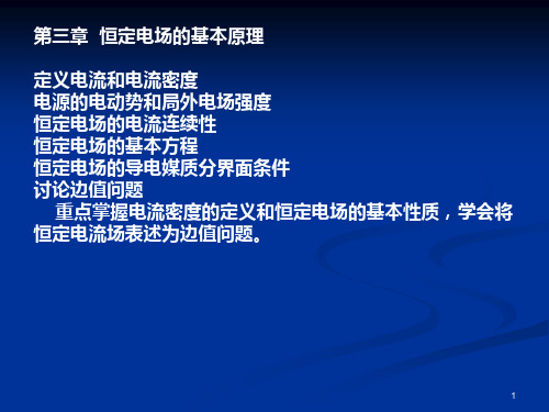
工程电磁场--第3章--恒定电场的基本原理

fe Ee lim qt 0 q t
q t 为试验电荷的电荷量。
19
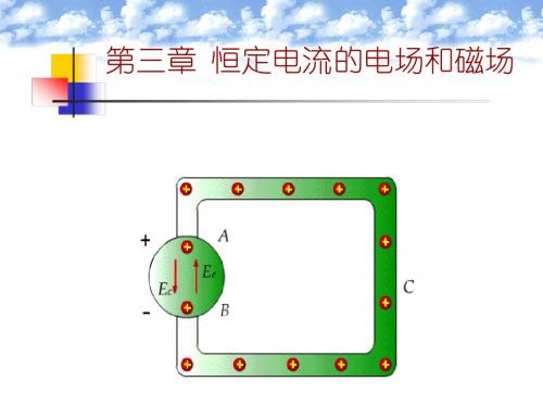
提供局外力的装置就是电源。 在电源中,其他形式的能量转换为电能。 在整个闭合回路中,电能又转换为别的 形式的能量。
20
2.电动势
下图是一个典型的导电回路, 蓝色部分为导 电媒质,黄色部分为电源。 电源中除库仑电场 外,还存在局外电场。 电源之外的导电媒 质中只有库伦电场。
0 1 E ex , D ex 1 x 1 x
自由电荷体密度
0 0 D ( )=2 x 1 x (1 x)
32
D E E E
E
E
E E E 2 E J 上式说明积累自由电荷的体密度与 的空间 变化有关。 对于均匀导电媒质,介电常数 和电导率 都
5
如果体积的厚度可以忽略, 可以认为电荷在面上运动,形成面电流。 密度为 的面电荷 以速度 v 运动, 形成面电流密度 K , 定义 K v 。 如图所示, db0 是垂直于 v 方向的线段元。
6
dl db0 dl dS dq dI K v dt dtdb0 dtdb0 dtdb0 db0
4
7
7
7
3
7
10 5
1.03× 10
7
10 15
16
3.2 恒定电场的基本方程
1.局外场
要维持导电媒质中的恒定电流,就必须有恒定 的电场强度。 (作用:克服运动中的阻力) 在电场的作用下,正自由电荷沿电场强度方向 运动, 负自由电荷沿相反方向运动。 对于金属导体, 主要是自由电子沿电场相反方向运动。
工程电磁场理论与应用讲义-3
第3章 电磁场分析的数学模型3.1 电磁场控制方程的表述电磁场数值分析的具体任务,就是要求解一个与特定问题相联系的偏微分方程定解问题。
根据数学物理方程的理论,所谓定解问题指的是在某一确定区域内成立的微分方程加上定解条件。
对于静态电磁场问题,或者可化为复数计算的正弦稳态电磁场问题,定解条件就是微分方程中的未知函数在该区域边界上所满足的条件,亦即边界条件;对于时变电磁场问题,则定解条件除了边界条件以外,还包括整个区域未知函数在初始时刻的值,亦即初始条件。
针对这一定解问题的求解,发展了如上节所述的各种解算方法。
因此,为了得到正确的解答,第一步工作就是要写出定解问题的表达式,也就是建立特定电磁场问题的恰当的数学模型。
定解问题中的偏微分方程通常称为控制方程。
选择哪种物理量作为控制方程中的未知函数,建立什么形式的微分方程,将影响问题求解的难易程度。
本节将从麦克斯韦方程组出发,介绍各种情况下电磁场控制方程的表述方式。
3.1.1 麦克斯韦方程组[54] 100多年前,麦克斯韦对前人在实验中得出的电磁场的基本定律进行了数学上的总结和提升,引入了位移电流的概念,创立了后来以其命名的方程组,完善了电磁场理论。
其著作《Treatise on Electricity and Magnetism 》成书于1873年。
从理论框架上看,麦克斯韦方程组加上洛仑兹力的计算公式,合起来构成了静止及运动媒质中电动力学的基础,概括了发电机、电动机和其它电磁装置的工作原理,也概括了电磁波的发射、传播和接收的原理。
科学技术发展的实践证明,描述电磁场宏观性质的麦克斯韦方程组正确反映了电磁场中各物理量之间的相互关系,是电磁场的基本方程。
在大学普通物理和电类专业的电工原理课程中,都对麦克斯韦方程组作了基本的介绍。
本节主要从电磁场数值计算的需要出发来加以说明。
麦克斯韦方程组的微分形式可以表述为:t∂∂+=⨯∇D J H (3-1) t∂∂-=⨯∇B E (3-2) 0=⋅∇B (3-3)ρ=⋅∇D (3-4)式中,H 、B 、D 、E 、J 、ρ 分别为磁场强度(A/m )、磁感应强度(或称磁通密度,T )、电位移(或称电通密度,C/m 2)、电场强度(V/m )、电流密度(A/ m 2)和电荷密度(C/ m 3)。
工程电磁场3

B
(a) 长直圆柱形铜导体截面
B
o
a
(b) 导体内、外|B|的变化曲线
图 无限长直圆柱形载流导体的磁场
0 I
2a
2
e
( a)
(2)导体外部( >a)
B dl 2B I
0 l
0 I B e 2
4.毕奥-萨伐尔定律
B(r ) (r ) A(r )
1 Br (r ) dV 0 4 V r r
0 J c 1 Br Ar dV dV 4 V r r 4 V R
2L
0 A ln ez ln ez ln e z 2 2 0 2
2L
Az B A 0 I e 2 e
0 I
例3-10:图示无限长直平行输电线,半径为a、线间距离为2b 且远大于a。试计算的矢量磁位和穿过输电线间单位长的磁通 量。 z
( a)
3.4.2 场分布:基于矢量磁位A
磁矢位 A 的引入 由
B 0 A 0 B A
A 称矢量磁位,单位: wb/m(韦伯/米)。
B 0 4
得
JdV eR 0 V R2 4
0 1 J dV= V 4 R
Q P1
M
B A
1 1 (sin A )er (rA )e r sin r r 0 a 2 I 0 a 2 I 2cos er sin e 3 3 4 r 4 r 0 m (2cos er sin e ) 3 4 r
3
工程电磁场知识点总结

工程电磁场知识点总结第一章矢量分析与场论1 源点是指。
2 场点是指。
3 距离矢量是,表示其方向的单位矢量用表示。
4 标量场的等值面方程表示为,矢量线方程可表示成坐标形式,也可表示成矢量形式。
5 梯度是研究标量场的工具,梯度的模表示梯度的方向表示。
6 方向导数与梯度的关系为7 梯度在直角坐标系中的表示为?u?。
8 矢量A在曲面S上的通量表示为?? 9 散度的物理含义是 10 散度在直角坐标系中的表示为??A?。
11 高斯散度定理。
12 矢量A沿一闭合路径l的环量表示为。
13 旋度的物理含义是 14 旋度在直角坐标系中的表示为??A?。
15 矢量场A在一点沿el方向的环量面密度与该点处的旋度之间的关系为。
16 斯托克斯定理17 柱坐标系中沿三坐标方向er,e?,ez的线元分别为,18 柱坐标系中沿三坐标方向er,e?,e?的线元分别为,19 ?1111???'??2eR?2e'R RRRR???20 ??????'??'???????4??(R)?R??R??11?0(R?0)( R?0)第二章静电场1 点电荷q在空间产生的电场强度计算公式为。
2 点电荷q 在空间产生的电位计算公式为。
3 已知空间电位分布?,则空间电场强度E。
4 已知空间电场强度分布E,电位参考点取在无穷远处,则空间一点P处的电位?P。
5 一球面半径为R,球心在坐标原点处,电量Q均匀分布在球面上,?则点?,,??处的电位等于。
222??RRR6 处于静电平衡状态的导体,导体表面电场强度的方向沿7 处于静电平衡状态的导体,导体内部电场强度等于 8处于静电平衡状态的导体,其内部电位和外部电位关系为 9 处于静电平衡状态的导体,其内部电荷体密度为 10处于静电平衡状态的导体,电荷分布在导体的。
11 无限长直导线,电荷线密度为?,则空间电场E。
12 无限大导电平面,电荷面密度为?,则空间电场E。
13 静电场中电场强度线与等位面14 两等量异号电荷q,相距一小距离d,形成一电偶极子,电偶极子的电偶极矩p= 。
工程电磁场-恒定磁场

例2 分析铁磁媒质与空气分界面情况。
μ0 α2
α1
μfe
铁磁媒质与空 气分界面
解:
tan 2
2 1
tan 1
0 fe
tan 1
0
2 0
表明 只要 1 90 ,空气侧的B
与分界面近似垂直,铁磁媒质表面
近似为等磁面。
2023/10/27
34/119
例 3 在两种媒质分界面两侧,
1 50,2 30
即 H2 H2yey H2xex 10ex 4ey A/m
B2 2H2 0(30ex 12ey ) T
M1 ∆l2
磁化电流是一种等效电流,是大量分子电流磁效应的表示。 有磁介质存在时,场中的 B 是传导电流和磁化电流共同 作用在真空中产生的磁场。
2023/10/27
20/119
4) 磁偶极子与电偶极子对比
模型
电量
电
偶
极
子
p qd
ρp - P p P en
电场与磁场
磁 偶
Jm M
极 子
Bx
0Ky 2
dx (x2 y2)
B
0K
2
ex
0K
2
e
x
y0 y0
2023/10/27
7/119
3.2 安培环路定律 Ampere’s Circuital Law 1. 真空中的安培环路定律
B dl l
l
0 I 2
e
dl
0I d l 2
0I
2
2
0 d 0 I
α
I dΦ
Bdl
解: 平行平面磁场,且轴对称,故
图3.2.19 磁场分布
工程电磁场第三章解读

3.1 Electric Flux Density
9. Example 3.1: find D in the region about a uniform line charge of 8nC/m lying along the z axis in free space. 10. Exercise: D3.1, D3.2
3. Electric Flux Density D (coulombs/square meter):direction (the
direction of the flux lines at that point) and magnitude (the number of flux lines crossing a surface normal to the lines divided by the S. area).
Ds S
The total flux passing through the closed surface is d closed Ds dS
surface
3.2 Gauss’s Law 4.To a gaussian surface, the mathematical formulation of Gauss’s law DS dS charge closed Q( Qn L dL S dS d )
4. Shown in the right figure
Q D r a a (inner ) 2 r 4a Q D r b a (outer ) 2 r 4b Q D a ( a r b) 2 r 4r
3.1 Electric Flux Density
工程电磁场第三章剖析
简单证明: 对J E 两边取面积分
左边 J dS I S
右边 E dS U dS S U GU
S
Sl
l
所以 U RI
7
3. 2恒定电场的基本方程 1. 局外场
要维持导电媒质中的恒定电流。就必须有恒定的电场强度。 在一个闭合回路中库仑电场的电场强度E闭合线积分为零。要维持恒定电流,电荷 在沿闭合回路运动时,还必须受到局外力的作用。
在电源中,除局外电场外,也存在库仑电场,故总的电场强度为 在电源以外的其他区域,只存在库仑电场,故总的电场强度
如果积分路径经过电源,则电场强度的闭合线积分等于电源的电动势
9
考虑电源以外的空间 电源以外的恒定电场是无旋场
10
3.电流连续性 根据电荷守恒原理,自然界中电荷量是守恒的。给定任意闭合面,设闭合面内的
密度为ρ的体电荷以速度v运动形成体电流密度J
穿过面积S的电流就是电流密度J在该面积上的通量
4
如果体积的厚度可以忽略,则可以认为电荷在面上运动,形成面电流,有面电流密度 如果面的宽度可以忽略,则可以认为电流在线上运动,形成线电流。
5
2.电流密度与电场强度的关系 要维持恒定电流,导电媒质中必须有电场强度。 电场强度也是恒定电场的基本场矢量。
积累自由电荷的体密度与 的空间变化有关。
14
• D • E • E • E • E • E
•
E
2
•
E
•
J
积累自由电荷的体密度与 的空间变化有关。
例 在均匀恒定电流场中,电流密度为1,沿 x 方向。 在 x 从 0 到 1 的区域,媒质电导率从1均匀增加到 2 , 介电常数保持 0 不变,试求自由电荷体密度。 解 据电流连续性,整个区域电流密度不随 x 变化,
工程磁场学第三章(2)
21
21
与 I 1 成正比。
M
I 21 1
M
21
21
I1
式中,M21 为互感,单位:H(亨利)
同理,回路2对回路1的互感可表示为
M
12
12
I2
可以证明
M
12
M
图3.7.5 电流I1 产生与回路2交链的磁链
21
互感是研究一个回路电流在另一个回路所产生的磁效应,它不仅与两个回路的
由 由
H 1t H
2t
,
得 得
1
I 2 r
I 2 r
sin
I 2 r
I
sin
I 2 r
sin
I cos
21 I
I I I
B1n B 2 n
cos 1
2 1 2 1
I
2 r
cos 2
dρ
外磁链
o
d
o
d
o
a
0I
2
ld ρ
0 Il
2
ln
b a
缆芯中的内磁链 i :
在距轴线为 的场点上的磁场强度为
H
i
1
2
2 a
2
I 2a
2
2
通过长度为1,宽为d’ 的面积元dS’ 与部分电流 链的元磁通
d
i
I
a
2
I
交
a
2
2
d
i
a
3
2
- 1、下载文档前请自行甄别文档内容的完整性,平台不提供额外的编辑、内容补充、找答案等附加服务。
- 2、"仅部分预览"的文档,不可在线预览部分如存在完整性等问题,可反馈申请退款(可完整预览的文档不适用该条件!)。
- 3、如文档侵犯您的权益,请联系客服反馈,我们会尽快为您处理(人工客服工作时间:9:00-18:30)。
The solution is easy if we can choose a surface, S, over which to integrate (Gaussian surface) that satisfies the following two conditions:
The integral now simplfies:
Engineering Electromagnetics
W.H. Hayt Jr. and J. A. Buck
Chapter 3:
Electric Flux Density, Gauss’ Law, and Divergence
Faraday Experiment
He started with a pair of metal spheres of different sizes; the larger one consisted of two hemispheres that cler sphere
q=0
A vector field is established which points in the direction of the “flow” or displacement. In this case, the direction is the outward radial direction in spherical coordinates. At each surface, we would have:
ground attached
Interpretation of the Faraday Experiment
q=0
Faraday concluded that there occurred a charge “displacement” from the inner sphere to the outer sphere. Displacement involves a flow or flux, existing within the dielectric, and whose magnitude is equivalent to the amount of “displaced” charge. Specifically:
Now, by a similar process, we find that:
and
All results are assembled to yield:
We know from symmetry that the field will be radially-directed (normal to the z axis) in cylindrical coordinates:
and that the field will vary with radius only:
We learned in Chapter 2 that:
It now follows that:
Gauss’ Law
The electric flux passing through any closed surface is equal to the total charge enclosed by that surface
Coaxial Transmission Line: Exterior Field
If a Gaussian cylindrical surface is drawn outside (b), a total charge of zero is enclosed, leading to the conclusion that
We now have:
and in a similar manner:
minus sign because Dx0 is inward flux through the back surface.
Therefore:
Charge Within a Differential Volume Element
Faraday Apparatus, Before Grounding
+Q
The inner charge, Q, induces an equal and opposite charge, -Q, on the inside surface of the outer sphere, by attracting free electrons in the outer material toward the positive charge. This means that before the outer sphere is grounded, charge +Q resides on the outside surface of the outer conductor.
…and the right hand side becomes:
Coaxial Transmission Line (continued)
We may now solve for the flux density:
and the electric field intensity becomes:
and the integral is set up as:
=
=
Another Example: Line Charge Field
Consider a line charge of uniform charge density L on the z axis that extends over the range z We need to choose an appropriate Gaussian surface, being mindful of these considerations:
C/m2
(0 < r <∞ )
We compare this to the electric field intensity in free space:
V/m (0 < r <∞ )
..and we see that:
Finding E and D from Charge Distributions
Faraday Apparatus, After Grounding
q=0
Attaching the ground connects the outer surface to an unlimited supply of free electrons, which then neutralize the positive charge layer. The net charge on the outer sphere is then the charge on the inner layer, or -Q.
So we choose a cylindrical surface of radius , and of length L.
Line Charge Field (continued)
Giving:
So that finally:
Another Example: Coaxial Transmission Line
So that:
Example: Point Charge Field
Begin with the radial flux density:
and consider a spherical surface of radius a that surrounds the charge, on which:
Mathematical Statement of Gauss’ Law
in which the charge can exist in the form of point charges: or a continuous charge distribution: Line charge:
Surface charge:
On the surface, the differential area is:
and this, combined with the outward unit normal vector is:
Point Charge Application (continued)
Now, the integrand becomes:
Point Charge Fields
If we now let the inner sphere radius reduce to a point, while maintaining the same charge, and let the outer sphere radius approach infinity, we have a point charge. The electric flux density is unchanged, but is defined over all space: