KISSsoft全实例中文教程1
KISSsoft全部课程(2024)

7
软件安装与启动
01
安装步骤详解
02
启动方法介绍
从下载软件安装包开始,逐步讲解安装过程中的各个步骤,包括选择 安装路径、配置系统环境等。
2024/1/29
介绍如何通过桌面快捷方式、开始菜单或命令行等方式启动KISSsoft 软件。
8
界面布局与功能介绍
2024/1/29
主界面构成
详细介绍KISSsoft软件的主界面 ,包括菜单栏、工具栏、项目树 、属性窗口等各个部分的功能和 作用。
操作项目。
详细讲解软件的系统设置,包 括语言设置、单位设置、精度 设置等,以满足不同用户的需
求和习惯。
10
03
齿轮设计课程
2024/1/29
11
齿轮类型与参数设置
03
齿轮类型
参数设置
齿轮材料选择
包括直齿轮、斜齿轮、锥齿轮、蜗轮蜗杆 等常见齿轮类型。
详细讲解模数、齿数、压力角、齿宽等齿 轮基本参数的设定原则和方法。
利用高级建模工具创建复杂的齿轮、轴承、轴等零部 件,并实现精确的装配。
参数化设计
通过参数化建模技术,快速生成系列化产品,提高设 计效率。
高级曲面造型
掌握高级曲面造型技术,创建复杂的曲面形状,实现 产品的流线型设计。
2024/1/29
32
高级仿真分析技术与方法
01
动力学仿真
利用高级仿真工具进行机构动力 学分析,研究机构的运动规律和 动态特性。
2024/1/29
响应面法优化
利用响应面法构建设计变量与目标函数之间的近似模型,实现高效优化。
34
THANKS
2024/1/29
35
传动系统的分类
验证圆柱齿轮的KISSsoft中文基础教程
验证圆柱齿轮的KISSsoft中文基础教程KISSsoft教程系列圆柱齿轮的计算 1. 设计任务本系列教程将介绍如何对已知数据的齿轮通过KISSsoft软件进行详细的分析和计算从而得出一系列的结果。
因此圆柱齿轮完整计算需要规定以下几个方面 1 所需原始的数据输入KISSsoft重新计算 2 按照DIN3990标准规范 3 根据实际要求创建文档的级别标准。
1.1 输入原始数据对于随后进行的数据输入说明请参阅本教程系列的第二章内容 1.1.1 载荷参数性能功率P 3.5 kw 驱主动速度n 2500 1/min 小齿轮 1 应用系数KA 1.35 寿命周期 750 h 1.1.2 几何法面模数mn 1.5 mm 斜齿螺旋角β 25 ? 度法面压力角 20 ? 度齿数 16/43 中心距a 48.9 mm 变位系数x 小齿轮1 0.3215 齿宽b 齿1/齿2 14/14.5 mm 1.1.3分度齿廓齿根高系数hfP 齿根半径系数齿顶高系数haP 齿1 主动轮 1.25 0.3 1.0 齿2 1.25 0.3 1.0 1.1.4附加数据材料 ? 材料硬度弯曲疲劳强度极限齿面接触疲劳极限齿1 主动轮 15 CrNi 6表面硬化 HRC 60 430N/mm2 1500N/mm2 齿2 15 CrNi 6 表面硬化 HRC 60430N/mm2 1500N/mm2 润滑脂润滑微量润滑油 GB00 80?C 基圆正切长度公差范围: 齿1 小齿轮 3 数最大基圆正切长度 Wkmax 最小基圆正切长度 Wkmin 齿11.782mm 11.758mm 齿2 6 25.214mm 25.183mm 质量Q DIN3961 8/8 2主要轮齿修形方法轮齿齿面轮廓修形线性和抛物线形接触方式正常不发生改变或不正确啮合小齿轮轴的性质图1.1 小齿轮轴的应变图 ISO 6336 图片13a I53mmS5.9mm dsh14mm 2. 解决方式 2.1 启动程序通常在注册以及安装之后通常的步骤有开始gt程序gtKISSsoft 04-2010gtKISSsoft才可以启动KISSsoft软件以下为整个操作的截图2.1 2.2 计算方式的选择在树型窗口下有一个活动的Module模块选择双圆柱齿轮副这样一个命令。
KISSsoft 渐开线花键强度计算【可用于车桥的制动凸轮轴、半轴、贯通轴花键的校核计算】
KISSsoft 渐开线花键强度计算
渐开线花键的计算,《机械设计》书中有简化的算法,有兴趣可以翻看下。
本例使用KISSsoft软件进行计算。
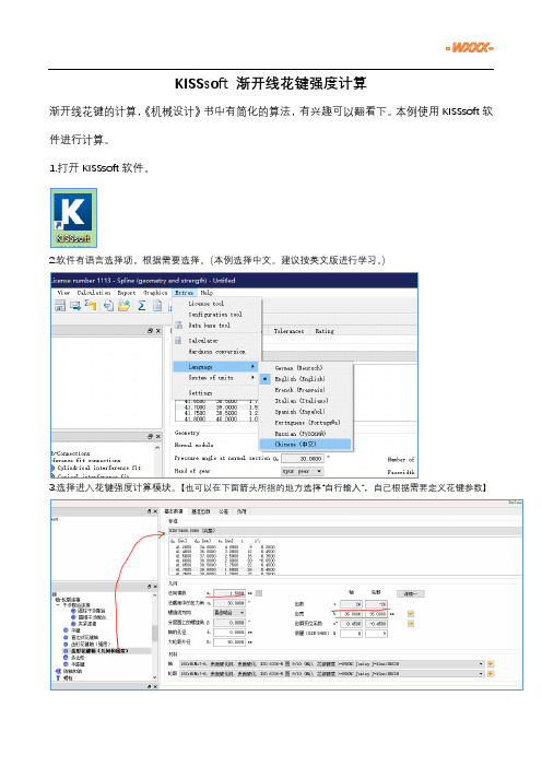
1.打开KISSsoft软件。
2.软件有语言选择项,根据需要选择。
(本例选择中文。
建议按英文版进行学习。
)
3.选择进入花键强度计算模块。
【也可以在下面箭头所指的地方选择“自行输入”,自己根据需要定义花键参数】
4.进入“负荷”标签栏,选择计算方法(默认是仅计算几何,需要根据需要选择强度计算的方法。
),填写载荷信息。
5.点击计算按钮,完成计算。
此时下边栏会出现计算结果概要。
6.点击“创建报告”按钮获得计算报告。
可以参考详细的计算结果。
【包含有应力信息和安全系数信息】
至此,简单的渐开线花键的强度校核流程就完成了。
【过程仅供参考,请自行购买专业的软件教程进行学习。
】。
KISSsoft全实例中文教程1

1.2 KISSsoft界面介绍在KISSsoft 03-2012程序内有4个的图标,具体的描述如图1-5所示。
选择启动应用程序图标,或者单击Windos任务栏【开始】→【程序】→【KISSsoft 03-2012】→【KISsoft】命令,启动KISsoft主程序,经过3秒钟左右进入界面。
图 1.5KISSsoft是一个windows兼容的软件应用程序。
普通Windows用户将认识到用户界面的元素,如菜单和上下文菜单、对话框、工具提示对接窗口、和状态栏、从其他应用程序。
因为在国际上有效的Windows风格指南是应用在开发期间,Windows用户会很快熟悉如何使用KISSsoft如图1-6所示:图 1.6经过中文翻译后如图1-7所示:图 1.71.3 材料KISSsoft自带材料库(Material Library),而且材料的种类比较多。
软件中材料库是根据计算单元分类。
比如轴计算是使用轴的材料库、螺丝计算是螺丝的材料库。
如果设计出现的材料KISSsoft库中没有,可自定义材料,一种是快速模块输入(不可重复利用),另一种是建立材料到材料库(可重复利用)。
在KISSsoft选择材料时要注意事项如下:1.同一种材料各国代号有所不同,比如45号中碳钢我国:45#、JIS:S45C、ASTM:1045、080M46,DIN:C45。
40Cr钢对应国外标准:JIS: SCr440、ASTM: 5140、ISO: 41Cr4。
2.同一种材料有KISSsoft多种热处理方式,选择时不要注意。
比如C45有C45(1)、C45(2)、C45(3),如图1.8所示。
都进行过热处理调质,但是最后C45(2)表面淬火、C45(3)表面氮化。
虽然抗拉强度一样,表面处理的不同会影响产品的抗疲劳与耐磨性能。
3. KISSsoft提供多种计算方法,因此同一种材料,在不同是计算标准下的性能可能有不同,比如:FKM、DIN、Hanchen等,根据实际情况提供一种计算标准所需的材料性能即可。
kisssys入门实例教程1
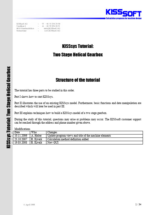
KISSsys Tutorial:Two Stage Helical GearboxStructure of the tutorial The tutorial has three parts to be studied in this order. Part I shows how to start KISSsys. Part II illustrates the use of an existing KISSsys model. Furthermore, basic functions and data manipulation are described which will later be used in part III. Part III explains techniques how to build a KISSsys model of a two stage gearbox. During the study of this tutorial, questions may arise or problems may occur. The KISSsoft customer support can be reached through the address and phone number given above. Modifications Date Who Changes 10.11.2006 A. Halter Update program views and title of the machine elements 23.10.2007 R. Kivelä Calculation method definition added 19.03.2008 R. Kivelä New GUIK I S S s y s T u t o r i a l : T w o S t a g e H e l i c a l G e a r b o xTable of content1Start KISSsys (3)1.1Start program (3)1.2Definition of project folder (3)1.3Opening a KISSsys model (3)2Toolbars and views (5)2.1Views in KISSsys (5)2.1.1Views and windows (5)2.1.2Arranging elements in the schematic (6)2.1.3Connection between 3D view, schematic and tree structure (6)2.1.4Using the 3D view (6)2.1.5Refresh All (6)2.2In- and output of data (7)2.3Starting KISSsoft analysis (7)3Using the model ...001-KISSsys-Tutorial“.. (8)3.1Calculate kinematics (8)3.2Analysis of root and flank safety factors (8)3.3Changing gear data, bearing data and shaft geometry (9)4Task (10)5Structure of the system (10)5.1Start KISSsys (10)5.2Loading the templates (10)5.3Principles (11)5.3.1Elements, templates (11)5.3.2Drag/Drop, Copy/paste, rename, delete (12)5.4Insert machine elements (12)5.5Definition of the kinematics (14)5.6Adding KISSsoft analysis modules (16)5.6.1KISSsoft shaft analysis (16)5.6.2Add KISSsoft gear analysis (17)5.6.3Adding bearing analysis (19)5.7Positioning the elements (19)5.7.1Preliminary positioning (19)5.7.2Positioning of the shafts (20)5.7.33D View (21)5.8Definition of the shaft geometry (22)5.9Definition of bearings (24)6User Interfaces (25)6.1Table with information on gear and bearing data (25)6.2User Interfaces (26)6.2.1Introducing an user interface (26)6.2.2Adding text (26)6.2.3Display of results (26)6.2.4Changing values using the “UserInterface” (29)6.2.5Changing calculation method from the “UserInterface” (29)6.2.6Further settings (30)6.2.7Execution of functions (31)7Completing the model (33)7.1Display of the coupling (33)7.2Definition of fixed and free bearings (33)7.3Definition of the force acting on the output shaft (34)PART I, Start KISSsys1Start KISSsys1.1Start programStart KISSsys through Windows-Start/Programs/KISSsoft 03-2008/KISSsys.1.2Definition of project folderKISSsys uses projects to manage the files. Project folder simply defines where KISSsys models and the respective KISSsoft files are saved. Before a KISSsys model can be opened or created, the project / folder where the model will be saved is to be defined.Using the button shown in the following figure, the project / folder selection is displayed, here “C:\Programs\KISSsoft 03-2008\KISSsys\Tutorial”. After having selected the project / folder, the selection is to be confirmed, press “Open” and KISSsys is launched.Figure1.2-1 Selection of project / folder1.3Opening a KISSsys modelAfter having selected the project, the KISSsys models available in this project can be opened through the menu using File/Open. The message whether the current file should be saved or not can be answered negatively since KISSsys starts with an empty file. Now, the KISSsys model KISSsys-Tutorial-001.ks is opened, and KISSsys should look as follows:Figure1.3-1 KISSsys after opening the model KISSsys-Tutorial-001.ksNote that models should be opened only from the current project.PART II, Using the Existing Model2Toolbars and views2.1Views in KISSsys2.1.1Views and windowsKISSsys features the following views:Tree structure Messages 3D View User Interface Tables SchematicFigure2.1-1 Views available in KISSsysThe tree structure, the schematic and the messages can be shown/hidden using the following buttons:Figure2.1-2 Show/hide tree structure, messages and schematicThe tables, user interfaces and 3D view can be minimised, restored and closed. Using the menu …Window“, navigating between the windows is possible. A closed window can be shown by a right mouse click on its corresponding element in the tree structure and then selecting “Show”.2.1.2Arranging elements in the schematicThe elements shown in the schematic can be arranged with the left mouse button.2.1.3Connection between 3D view, schematic and tree structureIf an element in the tree structure is selected (left mouse click), it is highlighted blue. Also, in the 3D view, a local co-ordinates system is shown in the centre of the element.Figure2.1-3 Selecting an element in the tree structure highlights it in the 3D viewIf an element is selected in the schematic, it is highlighted in the tree structure and in the 3D view.When moving the cursor over the elements of the schematic, the name of the respective element is shown. With a right mouse click, the element can be modified.Figure2.1-4 Information about the element in the schematic2.1.4Using the 3D viewIn the 3D view, the gearbox can be rotated, moved and zoomed (left, centre, right mouse buttons respectively).2.1.5Refresh AllData and graphics are updated when the …Refresh All“ button is pressed.Figure2.1-5 Refresh AllThis command results in an update of for example the 3D view after having changed some parameters such as the tip diameter of a gear or that the power flow is highlighted in the schematic after the calculation of the kinematics.2.2In- and output of dataIn the user interfaces and the tables, the following text elements are usedFeature Type UseBlack Output / text Using black, results are shown that change with theanalysis. Comments are also in black.Red Input In these fields, values can be entered directly or they canbe chosen from an underlying list (double click). Thevalues entered or chosen are then stored in the respectivevariables.Grey background Functions Functions are executed through double-click (left mousebutton)2.3Starting KISSsoft analysisThrough the tree structure, the KISSsoft analysis can be started by a double click on the respective symbols as shown below:KISSsoft bearing analysisKISSsoft bevel gear analysisKISSsoft chain drive analysisKISSsoft crossed helical gear analysisKISSsoft feather key analysisKISSsoft helical gear analysisKISSsoft interference fit analysisKISSsoft journal bearing analysisKISSsoft planetary gear analysisKISSsoft polygon analysisKISSsoft shaft analysis / graphical editorKISSsoft spline analysisKISSsoft splined shaft analysisKISSsoft toothed belt analysisKISSsoft v belt analysisKISSsoft woodruff key analysisKISSsoft worm gear analysisFigure2.3-1 KISSsoft analysis3Using the model …001-KISSsys-Tutorial“3.1Calculate kinematicsThe kinematic analysis is started through double click on the function …Kinematic“. All speeds, torques and bearing forces are calculated. Based on the input speed, the gear data and the output torque, the resulting reduction …i tot“, the input torque and the output speed are calculated and shown:Figure3.1-1 Results in the User Interface after execution of kinematics analysisThe speed at the input and the torque at the output can be defined directly. Note that the sign of the torque defines the direction of the power flow.After having changed the values for input speed and output torque, the kinematics should be analyzed again by executing the function …Kinematic“ in order to get the corresponding results.3.2Analysis of root and flank safety factorsOn execution of the function …Strength“ (double click) the kinematics are calculated again, followed by the strength analysis of the gears, bearings and shafts. The resulting safety factors for the root and flank are shown in the user interface (based on a lifetime of 20’000h):Figure3.2-1 Output of resulting safeties for root and flankIf the analysis is to be performed for a different lifetime, the required lifetime should be changed in KISSsoft. Using the function …GP1“, access to KISSsoft is available where the lifetime can be changed from 20 000h to e.g. 30 000h (repeat for second stage). In order to have the new value accepted, …Calculate F5” has to be pressed, then exit KISSsoft.:Figure3.2-2 Changing the required lifetimeAfter that, the calculation of the safety factors can be repeated by double click on …Strength“3.3Changing gear data, bearing data and shaft geometryThe gears, shafts and bearings can be changed in KISSsoft in the usual manner. For this, double click on a KISSsoft symbol in the tree structure in order to get into the KISSsoft analysis of the desired element. Here, for example fine sizing of gears can be executed or the type of bearing may be changed in the bearing analysis.In order to make the changes permanent, “Calculate F5” has to be pressed before exiting KISSsoft.Note that elements (gears, bearings, couplings, …) shown in the graphical shaft editor must not be removed or added since the number of elements on a shaft is defined in the tree structure within KISSsys.The number of elements to be arranged on a shaft may only be changed in KISSsys directly.PART III, Building a model4TaskIn KISSsys, a model of for the strength analysis of a two stage helical gearbox with analysis of the gears, bearings and shafts is to be built. This model is to be used for analysis or dimensioning such systems.In the end, the model built will correspond to the model …KISSsys-Tutorial-001”.5Structure of the systemThe new system will be built from elements like gears, shafts and couplings and the respective KISSsoft analysis modules. These elements and analysis modules will be imported from a library, called …Templates“.5.1Start KISSsysFirst a new project / folder is defined, e.g. C:\MyTutorial. Then, start KISSsys with this folder as project. KISSsys is then opened with an empty model. Using File/Save from the menu, this file is given a name, e.g. …KISSsys-Tutorial-001“.In order to be able to build a new model, KISSsys should be used in the administrator mode, which is activated in the Options - menu:Figure5.1-1 Change to Administrator modeIf the option …Administrator“ is not available, the respective license is missing. Contact KISSsoft AG.5.2Loading the templatesAs a first step when creating a new model, the templates are to be imported through the menu “File”, “Open templates…”, “templates.ks”.In the …Templates“, all elements available in KISSsys are now listed:Figure5.2-1 Element library …Templates“After having imported the templates, the model can now be assembled5.3Principles5.3.1Elements, templatesIn KISSsys, a model is assembled from different elements. These elements are arranged in a tree structure. The following types of elements are available:-Machine elements (red symbols)-Analysis modules for the respective machine element (light blue)-Connections (grey)-Tables-GraphicsThey are available from a library, called the templates. The templates may be modified by the user (recommended for experienced users only).The user can switch between the elements arranged in the tree structure and the template using the tabs asshown below or for easier use tabs can be arranged to be seen simultaneously:Figure5.3-1 Elements and templatesThe model is arranged in the …Model“ - section.5.3.2Drag/Drop, Copy/paste, rename, deleteUser can select how to copy elements from templates to the model. You may drag and drop elements or you can copy and paste elements from the templates to the tree structure using …Ctrl+C“ / …Ctrl+V“ or, with right mouse click, …copy“ / …paste“. Delete elements by selecting them and press “Del” or right mouse click and “Delete element”. Renaming an element is performed by right mouse click and selection of “Rename”.Note: Renaming an element will result in the connections to this element being invalid. Renaming elements is hence not recommended.5.4Insert machine elementsAll machine elements are arranged in a group. For this, the element …kSysGroup“ is imported from the “Templates” into the “Element” section. The name is changed to …GB“ for this example.The gearbox features three shafts. They are added by copying from the templates (element “kSysShaft”) and inserted in the group “GB”. They are called …s1“, …s2“ and …s3“. In the schematic, the shafts can be arranged using the left mouse. The model should look as follows:Figure5.4-1 View of the model after the first stepsNow, the other machine elements are integrated. They are arranged in the tree structure below their respective parent element (the respective shaft). First, the element …kSysCoupling“ is copied from the templates and pasted below …s1“ and below …s3“. Use the names …cIn“ for the coupling on shaft 1 (power input) and …cOut“ for the coupling on shaft 3 (power output). Similarly, on shaft 1 and 3, a single gear and on shaft 2 two gears are placed. They are copied from the templates, element …kSysHelicalGear“, and pasted below …s1“, …s2“ and …s3“. Use the names …z1“, …z2“, …z3“ and …z4“. The model should look as follows:Figure5.4-2 Couplings and gears addedNow, two roller bearings are included for each shaft. From the templates, the element …kSysRollerBearing“ is copied and pasted twice below each shaft. Use the names …b1“, and …b2“ in this example.On the output shaft (“s3”), a centric load is added. For this, the element …kSysCentricalLoad“ is copied from the templates and pasted below …s3“ and named as “f1”.The model should look as follows:Figure5.4-3 KISSsys model with all elements used5.5Definition of the kinematicsIn the next step, the kinematics and the power flow of the system is defined. For this, connections between the gears are introduced. For this the element …kSysGearPairConstraint“ is copied form the templates and pasted into the group …GB“ twice (names: …gp1“ and …gp2“). When inserting these connections a dialog appears where the two elements to be connected are selected:Choose first element of connectionChoose second element of connectionEfficiency (leave at 1.00)Figure5.5-1 Dialog for the definition of a gear-gear connection, left for the first connection called …gp1“, right forthe second connection called …gp2“In this example, the efficiency is to be left at 1.00.The definition of the power input is thorough the element …kSysSpeedOrForce“. For the input, paste the element on the same level as …GB“, using the name “Input”. Again, a dialog appears, where the connection to the coupling of the input shaft is defined. The input speed is defined as well by setting …Speed constrained“ to …yes“ and giving a value for the input speed:The Kinematics of the gearbox is defined by twoparameters, a speed and a torque.In this example, the speed on the input and the torque onthe output are defined. To set the speed on the input,choose …Speed constrained, yes“.Set …Torque constrained, no“ since the torque is definedfor the output, not for the input.The power is defined by the speed and the torque and isshown here for information.Figure5.5-2 Definition of the power inputFor the output, a second element …kSysSpeedOrForce“ is added, to be called …Output“. In the dialog, the coupling on the output shaft is to be selected as the connecting element. Here, the torque is to be given with e.g. -20Nm (…Torque constrained, yes“). Set a negative value for the torque to get a negative power.On the output, only the torque (with sign) is defined,…Torque constrained, yes“.The speed is not defined here, it is calculated based onthe gearbox kinematics and the speed on the input, hence…Speed constrained, no“.If a torque of +20Nm instead of -20Nm is used, thedirection of the powerflow in the gearbox is reversed.Figure5.5-3 Definition of the power outputThe symbols for the power input and output should be rearranged in the schematic.The KISSsys model should now look as follows:Figure5.5-4 KISSsys model with power flowDouble click on menu “Calculate kinematics” to start kinematics calculation. In the status line (bottom of the window), a message …Kinematic calculated“ occurs. There should be no error message.Figure5.5-5 Execution of kinematics analysisNote that the connections shown in the schematic have not turned red to indicate that power flows through them.Use “Refresh” button on menu to show power flow through the system. The information on the power flow is given with right mouse click on the element “Input” and selecting “Dialog”:Opposed to Figure5.5-2 not only the pre-defined speedat the input is shown but also the calculated torque. Figure5.5-6 Power input. The torque is calculated from the torque given for the input, the efficiency and thegearbox kinematicsThe analysis of the kinematics is now working.5.6Adding KISSsoft analysis modulesNext step is including the KISSsoft analysis modules. These are copied from the templates, …kSoftCalculations\withSystem”. KISSsoft analysis modules for shafts, bearings and gears are needed.5.6.1KISSsoft shaft analysisThe shaft analysis …Shaft“ is copied from the templates and pasted below the three shafts. They are called …S1“, …S2“ and …S3“. On pasting them, a dialog appears in which the shaft to be analyzed is to be selected. …Saving mode“ should set to …Save file in KISSsys“.Select the element for which the analysis will be usedThere are different ways to safe the KISSsoft analysismodules.With …Save file in KISSsys“, all data is saved in KISSsysThis is the most simple way. It is also possible to importor export KISSsoft files.Figure5.6-1 Dialog for definition of shaft to be analyzedThe KISSsys model should now look as follows:Figure5.6-2 Model with KISSsoft shaft analysis added for all three shafts5.6.2Add KISSsoft gear analysisFrom the templates, copy …HelicalGearPair“ and paste them below the two connections …gp1“ and …gp2“, using the names …GP1“ and …GP2“. Again, the analysis is connected to the connection using a dialog as follows. Set …Saving mode“ to …Save file in KISSsys“:Figure5.6-3 Dialog for definition of connection to be analyzed (gear stage)The KISSsys model should now look as follows:Figure5.6-4 Model with KISSsoft gear analysis addedThrough a double click on the KISSsoft gear analysis icon, the KISSsoft interface for definition of gears is shown. Here, gears can be defined in the usual way and the centre distance can be calculated. It is also possible to import gear data from an existing KISSsoft file for a gear pair. After having defined the gears, press “Calculate F5” and exit.Figure5.6-5 Definition of the two gear stages, here for stage 1This has to be done for both stages. Accept the input by pressing “Calculate F5” and close the KISSsoft window.5.6.3Adding bearing analysisThe bearing analysis …Bearing2“ is imported from the templates (index “2” since two bearings are to be analyzed). They are pasted below the three shafts, once per shaft. Names: …B_s1“, …B_s2“ and …B_s3“. In the dialog that appears, the shaft where the bearings to be analyzed are seated is to be selected. Set …Saving mode“ to …Save file in KISSsys“:Figure5.6-6 Selection of shaft where the bearings to be analysed are seatedWith this procedure, the KISSsoft bearing analysis is included. The KISSsys model should now look as follows:Figure5.6-7 KISSsys Model with all KISSsoft analysis modules (light blue icons) included5.7Positioning the elements5.7.1Preliminary positioningNext step: preliminary positioning of the parts on the shaft so that they can be identified more easily in the graphical shaft editor (when importing the elements from the templates, they all have position=0 mm). This step is not necessary to accomplish. For the bearings, gears and couplings, using right mouse click on the elements (…z1“ through …z4“, …cIn“, …cOut“ and all …b1“ and …b2“) and selecting …Properties“, the variable …position“ is available. Set the value for example to 10 mm for the left bearings (…b1“), 100 mm for the right bearings (…b2“), to 120 mm couplings on the output and input shaft, 120 mm for the force …f1“ and 30 mm and 70 mm for the gears.Example: left bearing on the input shaft:Figure5.7-1 Right mouse click on the element (here …b1“ below …s1“, the left bearing on the input shaft), select …Properties“A list with all variables available for the bearing appears. Set the value for the variable …position“ to 10:Figure5.7-2 Definition of the position of the left bearing to y=10 mmThis should be repeated for all elements. After pressing …Refresh“, the elements are shown in the correct order in the schematic:Figure5.7-3 Correct order of the elements in the schematic5.7.2Positioning of the shaftsThe shafts are still to be positioned with respect to each other. The second shaft should be parallel to the first shaft, the distance being the centre distance of the first gear pair. Shaft 3 should be parallel to shaft 2, and again in the distance of the centre distance of the second gear pair.Positioning procedure is started by right mouse click on …s2“ and …s3“, select …Dialog“:Figure5.7-4 Dialog for positioning of shaftsFirst, …s2“ is positioned with respect to …s1“. In the dialog, select …Parallel to Shaft“:Figure5.7-5 First part of the dialog, positioning with respect to an existing shaftIn the second part of the dialog, the shaft is positioned using a polar co-ordinates system. The distance between the two shafts (the radial co-ordinate) is equal to the centre distance of the first gear pair. The centre distance is available from the variable …GB.gp1.GP1.a“. The angle and the axial displacement are set to zero (no input required):In …Element“ reference element is selected.The starting point of the shaft (always it’s left end) to bepositioned can now be defined using polar or Cartesian co-ordinates. Easier is to use polar coordinates.The radial co-ordinate is equal to the centre distance of thegear pair 1 (= variable “GB.gp1.GP1.a”)Figure5.7-6 Second part of dialog, positioning of shaft 2 with respect to shaft 1To be repeated for shaft 3.5.7.33D ViewNow that all elements have been positioned (although only preliminary), the 3D view can be included (copy from templates, element …kSys3Dview“ and insert on the same level as the group …GB“). Using right mouse click and …Show“, the 3D view is shown as follows:Figure5.7-7 3D view of the systemThe shaft geometry and the bearings have not been defined yet.5.8Definition of the shaft geometryWith double click on the KISSsoft shaft analysis modules …S1“, …S2“ and …S3“ the KISSsoft shaft analysis is started. Here, in the graphical shaft editor, the shaft can be modeled in detail. When opening the shaft editor, no shaft is visible, only the elements positioned on the shafts are present. To keep it simple, a cylindrical element of diameter D=20mm and length 130mm is defined for all three shafts, shown here for the first shaft:Figure5.8-1 View when opening the graphical shaft editorAfter having inserted a cylindrical shaft:Figure5.8-2 View with cylindrical shaft addedThe shaft can now be detailed in the usual way. It is also possible to define bearings in shaft module including the axial supporting. After definition press …Calculate F5“ in order to start the shaft analysis. This is necessary to get reaction forces on the bearings which are in turn necessary for the bearing definition/analysis.This should be repeated for all three shafts (in this example, all shafts are 130 mm long and 20 mm, 30 mm and 40 mm in diameter. The 3D view changes as shown below when pressing …Refresh All“:Figure5.8-3 3D View with shaft geometry as defined5.9Definition of bearingsNow that all three shafts have been properly defined, the bearings can be defined. This order in defining the elements (shafts first, bearings second) is important since the inner diameter of the bearings is governed by the outer diameter of the shaft and the position of the bearing on the shaft.Double click on the bearing analysis (here using shaft 1 as example) …B_s1“, the respective KISSsoft analysis interface is shown. The inner diameter of the bearing is defined through the shaft diameter and the position of the bearing. Now, a suitable bearing can be chosen as usual.Figure5.9-1 Selection of bearing in KISSsoft for the given inner diameter of the bearing (=shaft diameter)After having chosen the bearing type and the bearing, press “Calculate F5” in order to activate the selection. To be repeated for all three pairs of bearings. The 3D view changes accordingly after pressing …Refresh All“:6User Interfaces6.1Table with information on gear and bearing dataFrom the templates, the following three tables can be copied into the tree structure below the group …GB“: …Bearing2Calculations“, …GearPairCalulations“ and …ShaftCalculations“:Figure6.1-1 Tables to be copied from the templatesOnce copied, using a right mouse click on the tables and pressing “Show” gives:Figure6.1-2 Tables with gear data, bearing data and KISSsoft gear pair analysis dataThese tables offer an overview over the parameters used. Parameters in red can be changed using the tables.6.2User Interfaces6.2.1Introducing an user interfaceA table for definition of the main input and output data is to be introduced: Choose the table …UserInterface“ from the templates and copy it into the tree using the name …UserInterface“. With …Show“, the table is shown. Use function “Dialog” to define the number of rows and columns for table size.Figure 6.2-1 Resizing a table6.2.2Adding textUse right mouse click and …Insert String“ to insert text as shown in the figure below. The text is to be defined in the field …Value“:Figure 6.2-2 Adding text to the user interfaceIf information in the field is only a text user can also directly write the information in the right field.6.2.3Display of resultsFirst, the speed at the output and the torque at the input (these values are calculated from the input values and the gear kinematics) are included in the user interface.With right mouse click, …Insert real“, the following dialog is shown. In …Expression“ the name and the path of the variable should be given. The speed at the output is given in the variable “speed”. Note that the full path “Output.speed” is to be given. Press “Ok” to accept and the result is shown in the user interface.Figure6.2-3 Showing the speed at the outputFigure6.2-4 Result in the user interfaceIn the same manner, the torque at the input is shown in the user interface. Right mouse click on the desired field, …Insert Real“, Expression: …Input.torque“, and the torque should be shown as follows:Figure6.2-5 Showing the torque at the inputSimilarly input and output powers can be shown. Furthermore, the total gear ratio shall be shown. Again, right mouse click on the desired field, …insert real“ and defining the following expression:Figure6.2-6 Calculation of the total reduction from input speed and output speedExpression is extended to have a condition (IF…THEN and ELSE) to check that Output speed is not zero to be able to evaluate the formula.。
KISSSOFT锥齿轮操作培训教材
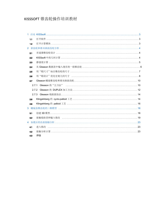
KISSSOFT锥齿轮操作培训教材1 启动KISSsoft (3)1.1打开软件 (3)1.2打开计算模块 (3)2 斜齿轮和准双曲面齿轮分析 (4)2.1差速器锥齿轮设计 (4)2.2KISSsoft中的几何计算 (4)2.3静强度计算 (5)2.4从Gleason数据表中输入现有的一组锥齿轮 (6)2.5用“粗尺寸”标注锥齿轮的尺寸 (7)2.6用“精设计”优化宏观几何尺寸 (8)2.7Gleason螺旋锥齿轮和准双曲面齿轮 (10)2.7.1 Gleason 的“五刀法” (10)2.7.2 Gleason 的DUPLEX 加工方法 (12)2.7.3 Gleason端面滚齿法 (14)2.8Klingelnberg 的cyclo-palloid 工艺 (14)2.9Klingelnberg 的palloid 工艺 (16)3 螺旋齿锥齿轮的三维模型 (18)3.1创建3D模型 (18)3.2接触线检查和输入修改 (19)4 加载后的齿面接触分析 (23)4.1进入修改 (23)4.2接触分析计算 (23)4.3评估1 .启动 KISSsoft 1.1 启动软件软件安装和激活后,您可以立即调用KISSsoft 。
通常,您可以单击“StartProgram Files KISSsoft 03-2017 KISSsoft 03-2017 ”启动程序。
这打开了 KISSsoft 软件用户界面:图1 KISSso 代软件用户界面1.2启动计算模块在计算模块中的相应条目中,双击启动“锥齿轮和准双曲面齿轮”计 算模块。
“模块”窗口位于主窗口左上角。
ModUefit5 K,TQQtihirfD *器 SiRegar、GEtwi g 谕.变』Pries wth rddk④ FHanetary gear 驾 Thrtfi oem tram 得 Frnr pearg trgn-nd 用gearj __ J F*cc gearsf Wgrms with en ,回眸ihg 甯 OiHsed helcd OMTE an ..名 Ngn GFQjfar gcfl-s■ Shaftsand Btamgs . Shaft CAlaiabC!^ ■ Rofcr ...8 Roierbwirtaiw/T^ i •图2从“模块”窗口中选择“锥齿轮和准双曲面齿轮”计算模块 2.锥齿轮和准双曲面齿轮分析I锥齿轮有各种不同的类型,每一种设计都有其独特的特点,必须加以 考虑。
齿轮Kisssoft全实例教程-2024鲜版

软件内置先进的齿轮分析算法,可对齿轮的强度、刚度、疲劳寿命等 进行精确计算,为设计者提供可靠的参考依据。
丰富的齿轮库
Kisssoft软件自带丰富的齿轮库,包含各种标准和非标准齿轮,方便 用户快速调用和修改。
灵活的参数化设计
软件支持参数化设计,用户可通过修改参数快速调整齿轮结构,提高 设计效率。
Chapter
2024/3/28
19
齿轮参数优化
选择齿轮类型
根据实际需求,选择适合的齿 轮类型,如直齿、斜齿、锥齿
等。
2024/3/28
确定齿轮参数
输入齿轮的模数、齿数、压力 角等基本参数。
优化设计变量
以齿轮的模数、齿数、变位系 数为设计变量,进行优化设计 。
目标函数设定
以齿轮的传动效率、噪声、振 动等性能指标为目标函数,进
实体建模与装配
分别将蜗杆和蜗轮的齿廓曲线 转化为三维实体模型,并进行 装配操作。
设计参数设置
包括模数、蜗杆头数、蜗轮齿 数、导程角等参数设定。
2024/3/28
蜗轮轮廓绘制
根据蜗杆的齿廓曲线和蜗轮齿 数,绘制蜗轮的齿廓曲线。
模型检查与优化
对装配后的模型进行干涉检查 、齿形修正等优化操作。
14
04
齿轮分析实例
查看分析结果
Kisssoft将生成详细的分析报告,包 括齿轮的强度、安全系数等关键指标 。
05
04
运行分析
启动Kisssoft的分析计算功能,对齿轮 进行强度分析。
2024/3/28
16
齿轮疲劳寿命分析
导入齿轮模型
与强度分析相同,首 先需要在Kisssoft中 导入齿轮模型。
选择疲劳寿命分析
kisssoft中文教程

本人刚刚接触kisssoft,鉴于目前中文资料少,特翻译了一点实例。
希望更多的高手们能写更多上乘的实例,推动新手更加快速的发展和成长。
1、soft是单个零部件sys是系统system的缩写(多个零件组成的部件)
2、启动kisssys
3、打开一个文件
帮助文档的路径
File—open---打开C:\Program Files\KISSsoft 03-2011\kisssys\tutorial\KISSsys-Tutorial-001.ks
4、调出视图窗口
显示和隐藏模型树、模板、信息kisssoft窗口等
去掉前面的钩子(对号),就可以隐藏相对应的部分。
添加对号,可以显示相应的部分。
5、示意图----反映了载荷传递的路径。
左击移动任何一个方框,箭头跟着一起改变。
6、模型树含义:(查看每一个轴和轴上;零部件的装配)
红色的S1表示第一个轴上的零件,第二个s1表示第1根轴.s是shaft轴的简写。
双击轴s1,弹出轴和轴上零部件的布置。
Z1、Z2、Z3、Z4、分别表示齿轮1 2 3 4.
B1、b2分别表示轴承1 2.标号顺序沿着载荷传递的路径。
可以编辑轴和轴上零部件的位置。
拖动轴承支架的位置。
直接关掉右上角窗口,返回到3D模型窗口
编辑轴后,更新减速器gear box。
6、运动学动力学计算Calculate kinematics
未完,待续。
- 1、下载文档前请自行甄别文档内容的完整性,平台不提供额外的编辑、内容补充、找答案等附加服务。
- 2、"仅部分预览"的文档,不可在线预览部分如存在完整性等问题,可反馈申请退款(可完整预览的文档不适用该条件!)。
- 3、如文档侵犯您的权益,请联系客服反馈,我们会尽快为您处理(人工客服工作时间:9:00-18:30)。
1.2 KISSsoft界面介绍在KISSsoft 03-2012程序内有4个的图标,具体的描述如图1-5所示。
选择启动应用程序图标,或者单击Windos任务栏【开始】→【程序】→【KISSsoft 03-2012】→【KISsoft】命令,启动KISsoft主程序,经过3秒钟左右进入界面。
图 1.5KISSsoft是一个windows兼容的软件应用程序。
普通Windows用户将认识到用户界面的元素,如菜单和上下文菜单、对话框、工具提示对接窗口、和状态栏、从其他应用程序。
因为在国际上有效的Windows风格指南是应用在开发期间,Windows用户会很快熟悉如何使用KISSsoft如图1-6所示:图 1.6经过中文翻译后如图1-7所示:图 1.71.3 材料KISSsoft自带材料库(Material Library),而且材料的种类比较多。
软件中材料库是根据计算单元分类。
比如轴计算是使用轴的材料库、螺丝计算是螺丝的材料库。
如果设计出现的材料KISSsoft库中没有,可自定义材料,一种是快速模块输入(不可重复利用),另一种是建立材料到材料库(可重复利用)。
在KISSsoft选择材料时要注意事项如下:1.同一种材料各国代号有所不同,比如45号中碳钢我国:45#、JIS:S45C、ASTM:1045、080M46,DIN:C45。
40Cr钢对应国外标准:JIS: SCr440、ASTM: 5140、ISO: 41Cr4。
2.同一种材料有KISSsoft多种热处理方式,选择时不要注意。
比如C45有C45(1)、C45(2)、C45(3),如图1.8所示。
都进行过热处理调质,但是最后C45(2)表面淬火、C45(3)表面氮化。
虽然抗拉强度一样,表面处理的不同会影响产品的抗疲劳与耐磨性能。
3. KISSsoft提供多种计算方法,因此同一种材料,在不同是计算标准下的性能可能有不同,比如:FKM、DIN、Hanchen等,根据实际情况提供一种计算标准所需的材料性能即可。
图-1.8说明:Actual reference diameter for Rp.屈服强度的实际参考直径,此时热处理时的毛坯直径以接近实际尺寸,留很少加工余量,否则对强度有较大影响。
常用轴和齿轮材料力学性能表:例:建立轴shaft材料40Cr。
建立一个全新的材料到轴材料库需要2个步骤:z定义基础材料Material basic data。
z定义轴材料。
说明:基础材料是以抗拉强度为基础的参数,并不能直接反应计算所需的疲劳强度,因此还需要在基础材料的基础上定义对应的计算所需疲劳强度。
比如轴计算的:弯曲、扭转、拉伸等疲劳强度,齿轮计算的接触、弯曲强度。
1.打开KISSSFOFT界面,单击基本参数工具按钮,如图1.9所示。
进入基本参数工具对话框。
基本参数工具可新建各种软件没有的轴承、材料、键等等。
图 1.92.注意:进入基本参数工具对话框,打开按钮时会有提示,是否开启基本参数工具写入功能,如图1.10所示。
否则无法定义材料,单击按钮Yes,进入下一个基本参数工具对话框,如图1.11所示。
图 1.10图 1.113.在基本参数工具对话框,选择Material basic data。
单击基本参数工具按钮Edit,进入基本参数工具对话框,如图1.12所示。
图 1.124.单击基本参数工具按钮。
进入编辑对话框,如图1.13所示,按图输入参数。
图 1.13图 1.135.完成输入后单击完成按钮OK,回到基本参数工具对话框,单击保存按钮Save,单击关闭按钮Close。
回到上一个基本参数工具对话框。
基础材料定义完成,接下来定义轴材料。
1.选择Material Shaft calculation。
单击基本参数工具按钮Edit,如图1.14所示。
进入基本参数工具对话框。
图 1.142.单击基本参数工具按钮Edit。
进入下一个基本参数工具对话框,如图1.15所示。
图1.153.单击基本参数工具按钮。
进入编辑对话框,如图1.16所示,按图输入参数。
图 1.164.完成输入后单击完成按钮OK。
回到基本参数工具对话框,单击保存按钮Save,单击关闭按钮Close。
完成40Cr材料的自定义。
快速模块输入法定义材料如下:1.在某个计算单元选择材料时,单击一个和计算所需性能比较接近的材料(如40Cr和34Crmo4接近),如图1.17所示。
然后勾选Own Input框选按钮,就可以直接修改原参数,如图1.18所示。
图 1.17图 1.181.4 载荷谱传动系统在实际工作中,有很大一部分情况受到的载荷是变化的,体现为扭矩和速度是变化的,不同档位所使用的频繁程度即每档所用时间也不相同,三者之间对应关系,就是载荷谱Load spectrum。
有了实际工作的载荷谱,即有了准确的设计输入条件,就可以得到传动系统各零件在载荷谱条件下的实际受力情况,从而可以得到比较准确的计算结果。
无载荷谱时,可以使用名义载荷乘以使用系数使用系数KA 确定计算载荷,无法准确测量时查表。
在kisssfot中如果使用变载荷谱,需对变载荷进行准确的描述,因此KA按照ISO6336和DIN3996要求需设置为1。
起重设备载荷级别组对应kisssfot载荷谱:载荷级别组载荷谱L1 轻偶尔承受最大载荷,经常承受轻载荷Load 1acc.DIN15020L2 中工作时间内轻、中、重载荷分布平均Load 2acc.DIN150203acc.DIN15020 L3 重经常承受最大载荷 Load某卷扬减速机最大输出扭矩Tmax=1000NM,转速25r/min。
对应的载荷谱DIN15020L1.L2、L3:某工程机械在工作时的载荷分布如下表,请建立载荷谱。
表载荷分布载荷速度r/min 扭矩Nm 使用率1 3000 200 20%2 2500 260 30%3 2000 300 40%4 1100 370 10%由于KISSSFOFT定义载荷谱只能以一个基数为标准,以倍率的形式指定其他载荷。
因此需要给出一个基数,比如以载荷谱中利用率最高的一个载荷3为基数,速度=2000r/min,扭矩=300Nm。
打开KISSSFOFT界面,单击基本参数工具按钮,如图1.20所示。
进入基本参数工具对话框,如图1.21所示。
图 1.20图 1.21在基本参数工具对话框,选择Load spectrum。
单击编辑按钮Edit,如图1.22所示。
进入基本参数工具Load spectrum对话框。
图 1.22单击基本参数工具按钮。
进入新建对话框,如图1.23所示,按图输入参数。
图 1.23完成输入后单击完成按钮OK。
回到基本参数工具Load spectrum对话框,单击保存按钮Save,单击关闭按钮Close。
如果要对某个载荷谱进行修改,选择后单击编辑按钮Edit。
验证载荷谱。
进入某个有选择载荷谱的计算单元,如圆柱齿轮副,如图1.24所示,输入功率基本参数,速度n=2000r/min,扭矩T=300Nm。
单击添加按钮。
进入定义载荷谱对话框,如图1.25所示,在载荷类型选择刚才建立的04 stage laod。
图 1.24图 1.25单击完成按钮OK。
回到定义载荷谱对话框,如图1.26所示,参数已更新和设计所需的载荷谱一样。
图 1.26不重复使用快速多载荷谱建立方法:1.进入某个有选择载荷谱的计算单元,如圆柱齿轮副,输入功率基本参数,速度n=2000r/min,扭矩T=300Nm。
单击添加按钮。
进入定义载荷谱对话框,如图1.27所示,在载荷类型选择Own Input(自定义)。
图 1.272.单击添加按钮。
进入确认载荷谱对话框,单击添加按钮,增加4行载荷数目,并修改参数,如图1.28所示。
图 1.29单击完成按钮OK。
回到定义载荷谱对话框,如图1.30所示,载荷谱参数已更新和设计所需的载荷谱一样。
图 1.30第二章圆柱销的计算圆柱销可以用来定位,传递动力和转矩,在安全装置中作被切断的保护件使用,如图2.1所示。
圆柱销安装要求:圆柱销依靠少量过盈固定在孔中,对销孔的尺寸,形状,表面粗糙度等要求较高,销孔在装配前须铰削。
通常被连接件的两孔应同时钻铰,孔壁的粗糙度不大于Ra0.6μm,一般实心销位置度0.03以下,弹性销0.2以下。
图 2.12.1相关资料圆柱销有普通圆柱销、内螺纹圆柱销、螺纹圆柱销、带孔销、弹性圆柱销等几种。
圆柱销目前多应用优质碳素结构钢为原材料制造。
一般情况下,材质多选用C35,C45,但须进行热处理,高强度销要求下选用轴承钢。
圆柱销有淬硬钢119.2、120.2和不淬硬钢119.1、120.1,材料有35#、45#、70#、GCr15、40Cr、35Crmo、42Crmo各种不锈钢等。
一般圆柱销普遍采用淬硬钢,销的材料、强度、硬度可以厂家协商。