Hydraulic Fracture
Modeling Ithaca’s natural hydraulic fractures
1INRODUCTIONHydraulic fractures occur naturally in the Earth’s crust. These range in size from mm as small pres-sure partings to km as magmatic dike intrusions. Ithaca, New York, which lies in the heart of the Fin-ger Lakes region, is a great place to see intermedi-ate-scale natural hydraulic fractures. Glaciation and erosion have led to large outcrops of middle and up-per Devonian clastic rocks. These rocks have ex-perienced two major orogenic events in addition to uplift and erosion all of which have left a pattern of brittle fracture in the rocks as seen today. A brief geological history of the area is necessary to set the stage for the discussion of natural hydraulic frac-tures in these rocks.Outcrops within the Finger Lakes are part of the Devonian Catskill Delta Complex, a clastic wedge that is more than 2 km thick in the Finger Lakes re-gion. The complex was deposited on a continental shelf with an open sea to the south and consists of layers of black shales, gray shales, silstones and sandstones, and an occasional limestone. Uplift ac-companying the Acadian orogeny to the east pro-vided a large source of sediment for the clastic wedge that was prograding into the Appalachian Ba-sin. Deposition rates reached 170m per Ma. At the close of the Paleozoic, during the Pennsylvanian and Permian, the Alleghanian orogeny caused wide-spread folding, faulting and jointing in eastern North America. This was the last major orogeny to affect this part of the continent.Engelder and others (see Engelder et al. 2000) have studied the joints and other geologic features within the Catskill Delta Complex for many years. There is an abundance of evidence that indicates that many of these joints developed as natural hydraulic fractures caused by abnormally high fluid pressures. The Alleghanian orogeny also left a unique imprint as many joints show a clockwise sequence in re-sponse to the reorientation of stress as the African continent collided with North America.There is a significant body of literature that de-scribes the joints and tries to interpret their origin and formation (e.g. Pollard & Aydin 1988). How-ever, there have been few numerical simulations to illustrate the theorized processes. The aim of this paper is to examine various components of these joints using numerical simulations to determine whether current formation theories are reasonable or valid.2GEOLOGIC EVIDENCE OF NATURAL HYDRAULIC FRACTURES AND STRESS ROTATIONSThe current theories of joint formation in the Cats-kill Delta Complex depend upon visual inspection of many joints and joint sets (Engelder et al. 2000). The first bit of evidence comes from the surface morphology of many of the joint surfaces in the silt-stone.Modeling Ithaca’s natural hydraulic fracturesB.J. Carter & A.R. IngraffeaCornell University, Ithaca, NY, USAT. EngelderPenn State University, University Park, PA, USAABSTRACT: Joints within the Catskill Delta complex are believed to be natural hydraulic fractures and abundant indirect evidence supports this claim. The indirect evidence is based on many observations of joint surface morphology and joint spacing among other features. The Alleghanian orogeny left a unique imprint on the joint surfaces also, indicating a rotating horizontal compressive stress field. Numerical simulations il-lustrate that the formation and propagation of the joints can be described by hydraulic fracturing mechanisms. The numerical simulations include hydraulic fracture propagation from sedimentary structures at layer inter-faces and fracture twisting in response to the reorientation of the remote stress field after initial joint propaga-tion.Cracks tend to start at points of higher stress con-centration (McConaughy & Engelder 2000). In the case of sedimentary beds, the largest stress concen-trations are in the form of concretions, fossils, rip-ples, groove casts, and similar features. Figure 1 shows a joint surface in the Ithaca Formation silt-stone that starts at a groove cast, a location where the siltstone penetrates the shale layer, formed dur-ing erosion of the muddy substrate and deposition of the silt. The figure also shows the plumose surface morphology of the joint surface. The plumose struc-tures and the related arrest lines are well described by Bahat & Engelder (1984). Barbs, the darkened lines in Figure 1, radiate from the plume axis and indicate the direction of fracture growth. Arrest lines mark the termination of crack propagation in-crements. Natural hydraulic fractures do not have a steady supply of fluid (Lacazette & Engelder 1992). As the crack propagates, the pressure decays and the crack arrests until the pressure builds up again.Figure 1. Plumose joint surface starting from a groove cast.It can also be seen in Figure 1 that the fracture initially stays within the siltstone layer. It has been found that in sedimentary basins where the horizon-tal stress is less than the vertical, the shale layers have a higher horizontal stress than the siltstones (Evans et al. 1989, Warpinski 1989). Assuming that the pore pressure is the same in both the shale and siltstone layers, then the fractures would form in the siltstones first. This will be more evident in the next figure.The difference in horizontal stress leads to joint-ing in the siltstones followed by jointing in the shale. Joints in the shale beds usually start at the edges of existing joints in the siltstone; the joints act as con-duits for the pore fluid. If there is no rotation of the principal horizontal stresses, joints will develop in the shale in plane with those in the sandstone. How-ever, if the horizontal stress does rotate, then en-echelon or fringe cracks will develop (Pollard et al. 1982). Figure 2 shows a set of fringe cracks that start at the interface between the siltstone and shale. These fractures propagate downward. The numer-ous small cracks at the immediate interface reduce to a few large cracks as propagation continues.Figure 2. Multiple en-echelon cracks propagate down from the siltstone-shale interface and are rotated from the parent joint.There are many more features of the joints that offer indirect evidence of natural hydraulic fractures, including joint spacing, slip on open joints, crosscut-ting and abutting relationships, and evidence of a pressure seal that could have led to over-pressurization of the formation. However, it is be-yond the scope of this paper to discuss all of this evidence. Instead, numerical simulations are used to illustrate that natural hydraulic fracturing processes can explain some of the features described herein.3HYDRAULIC FRACTURING SOFTWARE The 3D numerical simulations that are described in the following sections are performed using HY-FRANC3D and accompanying software (Carter et al. 2000a,b). In addition, ANSYS (ANSYS 2000) and FRANC2D (CFG 2000) are used for some 2D analyses.The 3D software consists of OSM, FRANC3D, HYFRANC3D, and BES. OSM is used to create the initial geometric models. FRANC3D is a fracture analysis code with pre- and post-processing capabili-ties. HYFRANC3D builds upon FRANC3D by add-ing a fluid flow module that couples the elastic structural response with fluid flowing in the fracture. BES is a linear elastic boundary element program. BES provides an elastic influence matrix that re-lates the set of unit pressures (p) at the nodes on the crack surface to the elastic displacements (w). The fluid flow formulation is based on the elasticity, lu-brication and continuity equations. For a Newtonian fluid, the stress ahead of the crack front has a 1/3 singularity, as does the fluid pressure inside thecrack (Carter et al. 2000b). Physically, the fluid pressure cannot be singular, thus, a fluid lag must develop at the crack front (Figure 3). The finite ele-ment formulation in HYFRANC3D combines an analytical solution for the pressure and crack open-ing displacement at the crack front with a standard finite element formulation of the lubrication equa-tion for the bulk of the fracture. The analytical solu-tion at the crack front provides an elegant way to overcome the singular behavior and limits the re-quired number of elements at the crack front. Hy-draulic fracture simulation proceeds as a series of crack advance increments, requiring an elastic solu-tion and coupled flow analysis at each step.Figure 3. Crack front region with fluid lag; p is pressure, w is crack opening displacement, V is crack front velocity, σ3 is clo-sure stress and x is the local coordinate axis along the crack.4SIMULATION OF HYDRAULIC FRACTURE PROPAGATION FROM A GROOVE CASTCracks tend to start at pre-existing flaws and points of high stress concentration. The groove cast in Fig-ure 1 is modeled to evaluate the stress intensification and to determine the hydraulic fracture propagation behavior from this location. The intent of these simulations is to show that hydraulic fracture is a plausible mechanism; thus, realistic boundary condi-tions are necessary, but accurate values are not es-sential to provide qualitative results.The numerical model consists of the siltstone layer only. McConaughy & Engelder (2000) de-scribe the difficulties in determining and modeling the correct boundary conditions. They conclude that the interface between the shale and siltstone must al-low slip. To simplify the 3D model, the upper and lower shale layers are notmodeled; a vertical con-straint is applied to the upper surface. A far-field compressive stress is applied in the horizontal direc-tion only; the vertical stress is neglected. The com-pressive stress perpendicular to the crack surface is 50 MPa and the stress parallel to the crack plane is 100 MPa. The elastic modulus is set to 14 GPa and the Poisson’s ratio is set to 0.1.The initial plane strain ANSYS stress analysis clearly shows that the groove cast alters the horizon-tal stress (Fig. 4). A tensile stress is induced at the groove cast. An initial crack is nucleated in the 3D numerical model at this location and hydraulic frac-ture propagation is simulated.Figure 4. ANSYS contours of maximum principal stress around a groove cast in a siltstone layer; tension is positive and values are in MPa.Figure 5 shows the shape of the hydraulic fracture after 17 steps of propagation. The fluid boundary conditions consist of a crack mouth flow rate equal to 1.0e-6 m3/s and zero flow rate at the crack front. These boundary conditions do not match the pre-sumed conditions of periodic fluidpressure build-up, but it is assumed that this will only affect the fracturing time and the surface features. The shape of the fracture to this stage matches that seen in the field reasonably well, although the barbs and arrest lines cannot be reproduced. The simulation can be continued such that the fracture breaks through the upper surface of the silt layer, but this is not com-plete yet.Figure 5. Shape of a hydraulic fracture from a groove cast af-ter 17 steps of propagation.5SIMULATION OF HYDRAULIC FRACTURE IN A ROTATING STRESS FIELDHydraulic fractures in these brittle rocks tend to grow perpendicular to the direction of maximum tension (or minimum compression). If an initial crack is subjected to a rotated stress field, the crack will kink out of the original plane to align itself with the new stress field. The rotation of the stress field induces different modes of deformation on different parts of the crack front. The kinking behavior de-pends on the pressure distribution inside the crack, the geometry of the crack, and the stress and stiff-ness contrasts in the rock layers (Carter et al. 1999). As a simple example, an initial elongated radial crack (emanating from a horizontal borehole) is ori-ented 70°from the maximum horizontal compres-sive stress (Fig. 6). The crack is nucleated in a single layer model with an elastic modulus of 27.6 GPa and a Poisson’s ratio of 0.25. The vertical stress is 69 MPa, the maximum horizontal stress is 62 MPa, and the minimum horizontal stress is 48 MPa. The crack mouth flow rate is set to 0.0795 m3/s.Figure 6. The initial crack shape is 9 m long and 0.3 m deep; σHmax is aligned with the x-axis (not to scale).Hydraulic fracture is simulated and stress inten-sity factors (SIF’s) are computed. Figure 7 shows the distribution of SIF’s along the initial crack front. The mode I values are highest, but there is a signifi-cant mode III component; mode II is significant only at the ends of the crack front. Pollard et al. (1982) provide a relationship between the mode III/I ratio and the number and spacing of en-echelon cracks that form along the crack front. Germanovich (2000) is conducting experiments on glass and brittle plastic to further characterize these relationships.The combination of all three modes is studied less well. However, the HYFRANC3D software allows the crack to propagate while ignoring the mode III SIF. Under these circumstances, the crack front does not break up, although, it quickly shows that it should. Figure 8 shows that the ends of the crack turn to align with σHmax. Most of the crack front is not aligned with σHmax. Instead, “large” ripples can be seen. The ripples are a result of the numerical propagation procedure, which only accounts for modes I and II. As the fracture propagates, the mode II and mode III SIFs increase rather than decrease. Due to the elongated shape, more effort is required to turn the entire crack front as compared to a more circular shape crack (Carter et al, 1999). As the crack front does not break, the combination of modes I and II produces initially minor oscillations in the crack front. These escalate as the crack con-tinues to grow, leading to the ripples.The mode III SIF value in the middle of the crack front reaches 10 MPa⋅√m at the final stage (15th step of propagation) while the mode I value remains rela-tively constant for each step, ranging from 20 to 25 MPa⋅√m along the crack front. Rotation and break up of the crack front is seen in many locations in the Ithaca area; Figure 9 shows a typical example.Figure 7. Mode I, II, and III SIF’s along the crack front; values are in MPa⋅√m.Figure 8. Ignoring mode III SIF during propagation leads to “large” ripples in the crack front indicating it should break up. The ends of the crack turn to align with the stress field.Figure 9. Joint in a siltstone indicating a rotated stress field as the crack surface shows obvious breaks; this might be seen as a set of en-echelon cracks when looking from above.6SIMULATION OF MULTIPLE HYDRAULIC FRACTURESMultiple parallel cracks tend to reduce in number and increase in spacing as they propagate. It is often assumed that the length to spacing ratio should be about 1.0 for a stable system of parallel cracks (Hwang, 1999). Figure 2 shows an example of a large number of closely spaced fractures at the shale-siltstone interface. As the cracks propagate down into the shale, most of the cracks arrest very quickly. Only a few, relatively widely spaced cracks remain at the base of the shale layer. Based on this figure, the length to spacing ratio is significantly greater than 1.0. Hwang (1999) has studied systems of parallel cracks, although not for 3D hydraulic fractures. Both 3D hydraulic fracture simulations and 2D simulations will be performed here.A set of three hydraulic fractures is used to gain insight into the behavior of a system of many paral-lel hydraulic fractures. The initial model is shown in Figure 10. The model is symmetrically constrained. The initial cracks are 1 mm deep and 6.35 mm apart. The crack mouth flow rate is 1.0e-6 m3/s and the material properties are the same as in section 4. In reality, more cracks should be modeled, but the simulations become quite time consuming as more cracks are added; three cracks should provide ade-quate insight.HYFRAN3D computes pressure distributions and crack opening displacements in the 3D fractures along with SIF distributions along the crack front. The usual procedure for growing multiples cracks is to scale the crack growth for all cracks based on the relative values of the stress intensity factors. Using this technique, the 3D hydraulic fractures are propa-gated for 10 steps. Although the mode I SIF for the center crack is slightly less than that for the two outer cracks (14.5 versus 15.2 MPa⋅√m for the initial crack), it continues to propagate. At step 10, the crack length is 10.5 mm. The length to spacing ratio is 1.7 and the center crack shows no signs of arrest-ing based on the relative mode I SIF values, 3.4 ver-sus 3.5 MPa⋅√m for the center and outer cracks re-spectively. Based on Figure 2, one might expect that the length to spacing ratio could be much higher than this. To verify that the crack growth is still sta-ble, 2D simulations are performed.FRANC2D is able to compute SIF’s, energy re-lease rates, and rates of energy release rates. The lat-ter allows the program to decide whether crack growth is stable and to decide which of the cracks are arrested. Although FRANC2D does not simulate fluid flow, a static pressure distribution of arbitrary shape can be applied to the crack surfaces (edges). It was shown previously (Carter et al, 1999) that if the correct pressure distribution, based on the 3D fluid flow analysis in HYFRANC3D, is applied to the crack surfaces of the 2D model, the correct hydrau-lic fracture behavior is captured. Thus, the pressure profile through the middle of each 3D crack is ap-plied to the 2D cracks to evaluate the rates of energy release rates.Figure 10. Initial 3D model of multiple parallel cracks.The initial FRANC2D analysis predicts that the center crack has a slightly lower rate of energy re-lease rate than the two outer cracks. The values are presented in matrix form in Table 1. The off-diagonal terms define the interaction between neighboring cracks. The negative values indicatethat crack growth is stable for all cracks. The influ-ence of neighboring cracks is relatively small, indi-cating a weak interaction.Table 1. Matrix of rates of energy release rate for 1 mm cracks.Crack 1 Crack 2 Crack 3 Crack 1 -0.6537E-01 -0.8141E-02 -0.2088E-02 Crack 2 -0.8141E-02 -0.6184E-01 -0.8141E-02 Crack 3 -0.2088E-02 -0.8141E-02 -0.6537E-01FRANC2D simulations corresponding to steps 5 and 10 of the 3D model are performed to examine the change in the rates as the cracks grow. The pres-sure profiles from the corresponding 3D HF simula-tions are used in the 2D simulations. The rates of energy release rate are provided in Tables 2-3. It is evident that the rate for the center crack is much less than the rate for the outer cracks at step 10, almost an order of magnitude. Also, the interaction between neighboring cracks is much stronger than for the ini-tial configuration. However, the rate is still non-zero and crack growth is still stable. The simulations are being continued to determine the final length to spacing ratio at which the center crack arrests.Table 2. Matrix of rates of energy release rate at 3.7 mm.Crack 1 Crack 2 Crack 3 Crack 1 -0.2531E-01 -0.5444E-02 -0.2027E-02 Crack 2 -0.5444E-02 -0.1514E-01 -0.5443E-02 Crack 3 -0.2027E-02 -0.5443E-02 -0.2534E-01Table 3. Matrix of rates of energy release rate at 10.7 mm.Crack 1 Crack 2 Crack 3 Crack 1 -0.1474E-01 -0.7807E-02 -0.4911E-02 Crack 2 -0.7807E-02 -0.2951E-02 -0.7807E-02 Crack 3 -0.4911E-02 -0.7807E-02 -0.1473E-017SIMULATION OF EN-ECHELON CRACKSEn-echelon cracks are often the result of crack front break up due to high mode III stress intensity fac-tors. The model in section 5 shows that the mode III stress intensity factor should not be ignored during propagation. Crack front break up is difficult to model, however, and is still not well understood.A simplified approach is taken here to examine crack front break up under a mode III loading. The model is shown in Figure 11. A single edge crack in a unit cube is subjected to a shear force while the crack faces are prevented from overlapping by the inclusion of a static fluid pressure. The elastic modulus is 10 GPa and Poisson’s ratio is set to zero. The SIFs are shown in Figure 12, which indicates the relatively high mode II and mode III SIF.Figure 11. Single edge crack subjected to mode III shear.Figure 12. SIF’s for single edge crack under torsion. Pollard et al. (1982) provide the following rela-tionship between the mode III/I ratio and the en-echelon crack orientation:()21tan211>−=−IIIIIKKKνβ(1)The inequality ensures an open crack. The equa-tion defines the orientation of a plane in front of the parent crack that has zero shear stress and the maximum tensile stress. If the mode III SIF is zero, the crack grows in its own plane. Based on the val-ues in Figure 12, β is –21° in the middle portion of the crack front. The initial spacing of the en-echeloncracks is less well defined and Germanovich (2000) continues to work on this.The initial crack front break up is modeled by manually creating a set of three small en-echelon “petal” cracks at the crack front as described by Germanovich (2000). Figures 13 and 14 show the side and plan views of the crack configurations. They are spaced 0.05 units apart with a radius of 0.02 units.Figure 13. Side view of 3 en-echelon cracks simulating the crack front break up.Figure 14. Plan view of 3 en-echelon cracks simulating the crack front break up.The initial stress analysis was performed without computing the elastic influence matrix. The maxi-mum principal stress is concentrated at the intersec-tion of the main and “petal” cracks (Figure 15). Ef-forts to define the crack growth criterion and propagation behavior for this crack configuration are continuing and further results will be presented elsewhere.Figure 15. Maximum principal stress is concentrated at the in-tersection of the main and “petal” cracks.8CONCLUSIONSThe indirect evidence for natural hydraulic fractures is abundant in the Ithaca, NY region. The proof might depend upon the interpretation, however. Numerical hydraulic fracture simulations lend addi-tional insight to the natural processes. Hydraulic fracture simulation from a sedimentary interface is modeled to examine the influence of natural stress concentrations, the propagation of multiple frac-tures, and the re-orientation of fractures in a rotating stress field.The simulations are not complete yet, but they do indicate that hydraulic fracturing is a plausible mechanism for describing the joints seen in the rocks in the Ithaca, NY region. The simulations are continuing and the final results will be presented later.ACKNOWLEDGEMENTSThe authors would like to acknowledge the past and present financial support of the NSF (EIA-9972853; EIA-9726388; CMS-9625406). This research was conducted using the resources of the Cornell Theory Center, which receives funding from Cornell Uni-versity, New York State, federal agencies, and cor-porate partners. Penn State’s Seal Evaluation Con-sortium (SEC) supported the fieldwork.REFERENCESANSYS 2000. /.Bahat, D. & T. Engelder 1984. Surface morphology on cross-fold joints of the Appalachian Plateau, New York and Pennsylvania, Tectonophysics 104:299-313.Carter, B.J., X. Weng, J. Desroches & A.R. Ingraffea, 1999.Hydraulic Fracture Reorientation: Influence of 3D Geome-try, Hydraulic Fracture Workshop, 37th US Rock Mechan-ics Symposium, Vail, CO.Carter, B.J., P.A Wawrzynek & A.R. Ingraffea 2000a. Auto-mated 3D Crack Growth Simulation, Gallagher Special Is-sue Int. J. Num. Meth. Engng. 47:229-253.Carter, B.J., J. Desroches, A.R. Ingraffea & Wawrzynek, P.A.2000b. Simulating fully 3d hydraulic fracturing. In M.Zaman, G. Gioda & Booker, J. (eds), Modeling in Geome-chanics, 525-557, Wiley Publishers.Engelder, T. & students 2000. The Catskill Delta Complex: Analog for modern continental shelf and delta sequences containing overpressured sections. SEC Report, Dept. of Geosciences, Penn State University.Evans, K., G. Oertel, T. Engelder 1989. Appalachian Stress Study 2: Analysis of Devonian shale core: some implica-tions for the nature of contemporary stress variations and Alleghanian deformation in Devonian rocks. J. Geophys.Res. 94:1755-1770.FRANC2D 2000. /software/. Germanovich, L. 2000. Pers. Comm.Hwang, C. 1999. Virtual crack extension method for calculat-ing rates of energy release rate and numerical simulation of crack growth in two and three dimensions. PhD Thesis, Cornell University, Ithaca, NY.Lacazette, A., & Engelder, T. 1992. Fluid-driven cyclic propa-gation of a joint in the Ithaca siltstone, Appalachian Basin, New York, in B. Evans & T-F. Wong, (eds.), Fault me-chanics and transport properties of rocks. 297-324, Lon-don: Academic Press Ltd.McConaughy, D.T. & Engelder, T. 2000. The nature of stress concentrations associated with joint initiation in bedded clastic rocks. Journal of Structural Geology (in press). Pollard, D.D. & Aydin, A. 1988. Progress in understanding jointing over the past century. Geological Society of Amer-ica Bulletin, 100:1181-1204.Pollard, D.D., P. Segall & P.T. Delaney 1982. Formation and interpretation of dilatant echelon cracks. Geol. Soc. Bull.93:1291-1303.Warpinski, N.R. 1989. Determining the minimum in situ stress from hydraulic fracturing through perforations. Int. J. Rock Mech & Min. Sci. 26:523-532.。
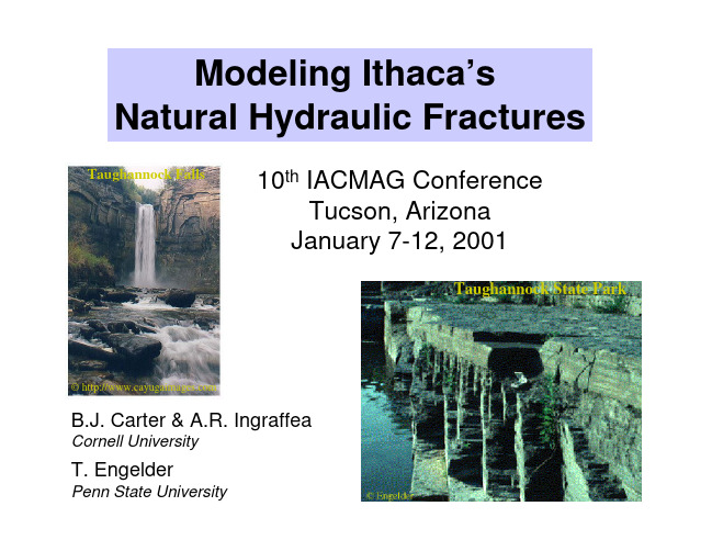
Modeling Ithaca’s Natural Hydraulic Fractures-ppt
Sequence of fracturing
• Jointing in the siltstone occurs before jointing in the shale; horizontal stress is lower in the siltstone because the shale compacts more. • Joints act as conduits for the pore fluid. • Joints in the shale are in plane with the siltstone joints unless the stress field rotates, which leads to en-echelon crack patterns.
Watkins Glen, NY
Taughannock Falls 215 ft high
©
Evidence of Natural Hydraulic Fracturing
• Crack surface morphology indicates periodic crack growth and arrest. • Many closely spaced multiple cracks initiate and propagate from a single source. • Fractures initiate in the siltstone first, followed by fracturing of the shale. • Organic rich sediments (black shales) are capable of producing natural gas or fluids. • Presence of a paleo-pressure seal could induce abnormally high pressure. • Shear displacement of joint surfaces occurs without shear deformation surface features.
页岩储层水平井密切割压裂射孔参数优化方法
Finallyꎬ a reasonable and comprehensive perforating parameter optimization method was developed for horizontal
well multi ̄cluster fracturing in shale reservoirs. The results show that more perforation clusters in a single stage
limited extentꎬ and an excessive reduction of perforation number may lead to very high operation pressure. With δ v
≤0 01 as the targetꎬ this optimization method was applied to two example wells to optimize perforating parameters
缝是否扩展和扩展方向ꎮ
平井的生产测井数据发现ꎬ 大约有⅟
的射孔簇在压
1 1 岩石变形方程
同时ꎬ 国内威远、 长宁、 昭通和焦石坝页岩气田或
扰相邻水力裂缝的扩展行为ꎮ 为准确考虑多裂缝同
示范区页岩气生产井产量差异也很大ꎬ 近半数射孔
步延伸过程中缝间应力干扰的影响ꎬ 采用二维位移
裂后贡献了
的产量ꎬ 而约⅟
开发工程国家重点实验室开放基金项目 “ 陆相页岩气水平井密切割暂堵均衡压裂控制机理与优化研究” ( PLN2021-09) ꎮ
Copyright©博看网. All Rights Reserved.
— 90 —
2023 年 第 51 卷 第 6 期
掘进机的专业单词
full face rock TBM with reaming type 扩孔式
全断面岩石隧道掘进机
full face rock tunnel boring machine 全断面岩
石隧道掘进机
G
gallery 坑道,地道,廊道
gauge cutter 边滚刀
gunite 喷射混泥土,喷浆准仪
H
hardener 硬化剂,固化剂
hardening agent 硬化剂,固化剂
crushing strength 抗压强度
crystalline rock 结晶岩
cut 掏槽,切割
cut blasting 掏槽破裂
cutter 滚刀,刀具
cutter axial spacing 轴向刀间距
cutter edge angle 刀刃角
连续变形分析
deflectometer 挠度计
deformation modulus 变形模量
degree of fissures 裂隙频度,裂隙率
delayed deformation 延时变形
detonation 爆炸,起爆
detonation wave 爆炸波
bench mark 水准点,基点,测量标点
bending stress 弯曲应力
bending test 弯曲实验
birefringence method(of measuring residual
stress) 双折射法(测量岩体残余应力)
block theory 块体理论
cutter head 刀盘,切削头
cutterhead bearing 刀盘轴承
Teton坝

13
谢谢
14
水利工程中土石坝失 事的典型案例—— teton坝(美国)
1
简介
不要小看渗透破坏,我们98年九江口决堤就是因为水力劈裂造成的管涌! 那什么是水力劈裂呢? ——hydraulic fracture
2
水力劈裂 hydraulic fracture Nhomakorabea
水力劈裂:又称渗透变形,当水力梯度超过 一定的界限值后,土中的渗流水流会把部 分土体或土颗粒冲出、带走,导致局部土 体发生位移,位移达到一定程度,土体将 发生失稳破坏,这种现象称为渗透变形。 水力劈裂主要有二种形式: (1) 流土(砂):渗流水流将整个土体带走的 现象。 (2) 管涌:渗流中土体大颗粒之间的小颗粒 被冲出的现象,可以发生于局部范围,但 也可能逐步扩大,最后导致土体失稳破 坏。——teton 坝
破坏时间间隔很 短,——渗透破 坏具有突然性
10
坝底的设施几乎被彻底摧毁
11
水力劈裂(管涌)后果不容小视
12
如何防止水力劈裂?hydraulic fracture
(1)控制土石坝设计条件 :由于水力劈裂机理分析可知坝中存在低应力区可 导致水力劈裂的产生。 因此,设计中应努力消除不均匀沉降的因素,以避免 坝内产生低应力区。 (2)控制水库运行条件 :大量资料表明,在水库初次蓄水至最高水位,且蓄 水速率较快时最容易引起土石坝水力劈裂。这是由于蓄水初期,坝体还未来得 及在自重下充分固结,土体内的有效应力还不足以阻止库水压力的劈裂作用。 另外,蓄水速率较快时,坝体中某些原先就存在的裂缝来不及愈合就被库水压 力劈开。相反,若蓄水速率较慢,库水能充分渗入周围的土体就不可能形成劈 缝压力。因此,在水库初次蓄水时,应限制蓄水速率不要太快,同时要严密监 视土石坝的表现。 (3)优选防渗体土料 :防渗体土料应避免用分散性土或易冲蚀性土,以防止 水力劈裂引起的初始渗漏导致垮坝失事,尽量减小不均匀系数。 (4)在防渗体下游侧设置反滤层:当水力劈裂缝形成时,下游反滤层可使防 渗体免遭渗透水继续冲刷,保证大坝安全。 总之,危害土石坝安全的最主要因素是渗流破坏。水力劈裂是导致土石坝因集 中渗漏而失稳的可能原因之一。只要从土石坝设计条件和水库运行条件两方面 加以控制采取必要措施,就可保证土石坝不因水力劈裂而造成破坏。
Simulating Fully 3D Hydraulic Fracturing

Simulating Fully 3D Hydraulic FracturingB.J. Carter†, J. Desroches‡, A.R. Ingraffea†, and P.A. Wawrzynek††Cornell University, Ithaca, NY‡Schlumberger Well Services, Houston, TX1.0 IntroductionHydraulic fracturing, the process of initiation and propagation of a crack by pumping fluid at relatively high flow rates and pressures, is one of several techniques for creating cracks in rock. Fractures in the earth's crust are desired for a variety of reasons, including enhanced oil and gas recovery, re-injection of drilling or other environmentally sensitive wastes, measurement of in situ stresses, geothermal energy recovery, and enhanced well water production. These fractures can range in size from a few meters to hundreds of meters, and their cost is often a significant portion of the total development cost. In locations where the in situ stress field, including the directions, is known and the wellbore is aligned with one of the far-field principal stresses, the hydraulic fracture geometry can be predicted and controlled with reasonable accuracy. For those wellbores that are not aligned with such a direction (deviated wells), the hydraulic fracture geometry is usually more complex and more difficult to model, especially close to the wellbore where the local stress field is significantly different from the far-field stresses. Field data from hydraulic fracturing operations exist primarily in the form of pressure response curves. It is difficult to define the actual hydraulic fracture geometry from this data alone, however. Therefore, numerical simulations are used to evaluate and predict the location, direction and extent of these hydraulic fractures.Simulations range from two to fully three dimensional depending on the degree of complexity of the wellbore and fracture geometries, the capability of the available simulator, and the required accuracy of the predictions. Numerous 2D, pseudo-3D, and planar 3D hydraulic fracturing simulators exist, and these simulators work very well in many cases where the geometry of the fracture is easily defined and constrained to a single plane. However, there are instances where a fully 3D simulator is necessary for more accurate modeling. For example, fractures from deviated wellbores are generally non-planar with arbitrary crack front shapes. Most hydrofracturing simulators simply ignore the near-wellbore effects of deviated wells and assume a planar starting crack that has extended beyond this region. The problem with this approach is that most of the difficulties and failures in hydraulic fracturing of deviated wellbores can be attributed to restricted flow in the near-wellbore region. Restricted flow usually is due to fracture reorientation and interaction with other fractures. Hydraulic fracturing of deviated wells, where the fractures reorient as they propagate, clearly requires fully 3D simulation capabilities and accurate modeling of the near-wellbore geometry.Efficient numerical simulation of fully 3D hydraulic fracturing requires at least two key components. The first is a capability for representing and visualizing the complex wellbore and fracture geometries. The second is a method for solving the highly non-linear coupling between the equations for the fluid flow in the fracture and the deformation and propagation of the fracture. The first component can be partitioned into several sub-components, including geometrical and topological solid modeling tools, routines to model geometry and topology changes for fracture propagation, automated meshing and remeshing capabilities, visualization ofresponse information, and analysis control information (i.e. input for a stress analysis program). The second component consists of a stress analysis procedure, fluid flow simulation capabilities, and a method for coupling the structural response with the fluid flow, including rules for determining hydraulic fracture propagation direction and extent. The authors have developed a simulator that includes all of these components for modeling multiple, non-planar, fully 3D, hydraulic fracture propagation. This simulator treats hydraulic fracturing as a quasi-static process, and the solution consists of a series of “snapshots in time” of the fracture geometry, fluid pressures, and crack opening displacements.A brief history of hydraulic fracturing and the development of hydrofracturing simulators are discussed in the next section. Then the key components of the new simulator are described in some detail, including the software framework for model representation, the coupled elasticity and lubrication theory, the finite element implementation of this theory, and the iterative solution procedure. The simulator has been verified for a radial (penny-shape) and a slot-like (part-through) fracture by comparing results to those from a robust and accurate 2D simulator, Loramec (Desroches and Thiercelin, 1993). Further simulations that compare well with experimental results show the ability of the system to model more realistic hydraulic fracture geometries. This chapter concentrates on the development of the simulator rather than actual simulations, however. Detailed simulations of hydraulic fracturing from cased, perforated, deviated wellbores is possible now, but is computationally intensive and is left as the subject of future publications.2.0 BackgroundThe process of hydraulic fracturing is not new. Nature has produced many such fractures in the earth's crust (see for example Bahat, 1991). The first recorded application of hydraulic fracturing for enhancing oil recovery that the authors are aware of was in 1947 in Kansas (see Howard and Fast, 1970). The "Hydrafrac" concept was formalized first by Clark (1949), although others had recognized previously that "pressure parting" could occur during acid treatment and water injection, a phenomenon considered to be closely related to the "Hydrafrac" concept (Howard and Fast, 1970). The Hugotan field in western Kansas was the site of the first hydraulic fracturing operation, and by the mid-1960's, hydraulic fracturing had become the dominant method of stimulation in this and many other fields (Howard and Fast, 1970).During this early period of hydraulic fracturing, two simple models were proposed to try to predict the shape and size of a hydraulic fracture based on the rock and fluid properties, the pumping parameters, and the in situ stresses (Khristianovic and Zheltov, 1955; Geertsma and de Klerk, 1969; Perkins and Kern, 1961; Nordgren, 1972). The models are known as the KGD and PKN models, and their description can be found in the above references and in many other summaries or texts (eg. Geertsma, 1989; Mendelsohn, 1984a,b). Perkins and Kern (1961) and Geertsma and de Klerk (1969) also derived a model for radial hydraulic fracturing. The radial, KGD, and PKN models are essentially two dimensional plane strain formulations with fluid flow only along the length (or radius) of the fracture. The fracture width and shape are related to the fluid pressure distribution in the fracture; the KGD model has a constant height and constantwidth through the height, while the PKN model has a constant height and an elliptical vertical cross-section.The 2D models are not able to simulate both vertical and lateral propagation. Therefore, pseudo-3D models were formulated by removing the assumption of constant and uniform height (Settari and Cleary, 1986; Morales, 1989). The height in the pseudo-3D models is a function of position along the fracture as well as time. The major assumption is that the fracture length is much greater than the height, and an important difference between the pseudo-3D and the 2D models is the addition of a vertical fluid flow component. The pseudo-3D models have been used to model fractures through multiple rock layers with differing stresses and properties. These models are simple, fast, and relatively effective. Warpinski et al. (1994) recently provided brief descriptions and a comparison of predictions for a number of simulators, including 2D and pseudo-3D models.Pseudo-3D models cannot handle fractures of arbitrary shape and orientation, however; fully 3D models are required for this purpose. The literature contains numerous references to fully 3D simulators; the majority of these are limited to planar fracture surfaces, however. These are called planar-3D simulators in this chapter to differentiate them from true fully 3D simulators which can model out-of-plane fracture growth. Planar-3D simulators have been developed by Clifton and Abou-Sayed (1979), Barree (1983), Touboul et al. (1986), Morita et al.(1988), Advani et al. (1990), and Gu and Leung (1993). Out of plane 3D hydraulic fracture growth has been modeled by Lam et al. (1986), Vandamme and Jeffrey (1986), and Sousa et al. (1993). To the authors’ knowledge, only Carter et al.(1994), using the predecessor of the simulatordescribed herein, have modeled 3D fracture in the near-wellbore region of a cased, perforated, and deviated wellbore.The increasing use of deviated wellbores implies that fully 3D hydraulic fracture simulators are vital to the petroleum industry. Hydrofracturing is often less effective for deviated wellbores as compared to traditional vertical wells. Some of the problems have been attributed to a poor understanding of the mechanics of fracture initiation and propagation from a deviated wellbore. The complex state of stress which is generated around an inclined wellbore (Yew and Li, 1988; Ong and Roegiers, 1995) means that the fracture propagates with a complex geometry (Behrmann and Elbel, 1990; Hallam and Last, 1991; Weijers and de Pater, 1992; Abass et al., 1996). The complex stress state and fracture geometry can limit the fracture width at the wellbore and hinder the injection of proppant into the fracture leading to premature screenout (Hallam and Last, 1991; Soliman et al., 1996). Nevertheless, the advantages of drilling inclined wellbores are significant. For example, the ability to drill several wells from a single location minimizes production infrastructure and impact on the environment. Therefore, the ability to model hydraulic fracturing from deviated wells is of ever increasing importance.In addition to inadequate modeling of the fracture geometry, many of the current hydraulic fracturing simulators do not predict the correct wellbore fluid pressure or fracture geometry even for planar fractures. The proposed reasons for this are numerous (Medlin and Fitch, 1983; Warpinski, 1985; Shlyapobersky et al., 1988; Jeffrey, 1989; Palmer and Veatch, 1990; Johnson and Cleary, 1991; Gardner, 1992; Papanastasiou and Thiercelin, 1993; de Pater et al., 1993 and van den Hoek et al., 1993). The simulator developed here addresses this problem by properlymodeling the near crack tip behavior (SCR, 1993). Furthermore, the simulator is ideal for modeling non-planar hydraulic fracturing, and is able to model multiple branching, intersecting, and merging fractures as will be shown in the following section.3.0 Model RepresentationThe first key component of an efficient, fully 3D, hydraulic fracture simulator is the geometric representation of the model. Representation implies computer storage and visualization of the model topology and geometry. This portion of the hydraulic fracture simulator is actually a general purpose, fully 3D, fracture analysis code, called FRANC3D, under development at Cornell University since 1987 (Martha, 1989; Wawrzynek, 1991; Potyondy, 1993). FRANC3D is capable of modeling multiple, arbitrary, non-planar, 3D cracks in complex structures, and has pre- and post-processing capabilities for both finite and boundary elements. It relies on a boundary surface representation of the model and a radial edge data structure for storing and accessing topological and geometrical information. It has the ability to do fully automatic or fully user-controlled crack growth simulations, including post-processing of the response information, modifying the geometry, remeshing, and updating the boundary conditions for each stage of crack growth. The complex geometry associated with perforated, cased, and deviated wellbores with multiple non-planar evolving 3D cracks requires a sophisticated, but easy to use simulation capability. FRANC3D has these capabilities, and some of its individual components are described briefly in the following sections.3.1 Representational Model of Fracture PropagationCrack growth simulation in FRANC3D is an incremental process, where a sequence of operations is repeated for a progression of models (Figure 1). Each step in the process relies on previously computed results and represents one crack configuration. There are four primary collections of data, or databases, required for each step. The first is the representational database, denoted R i(where the subscript identifies the step). The representational database contains a description of the solid model geometry, including the cracks, the boundary conditions, and the material properties. The representational database is transformed by a discretization (or meshing, M) process to a stress analysis database A i. The analysis database contains a complete, but approximate description of the body, suitable for input to a solution procedure (S), usually a finite or boundary element stress analysis program.The solution procedure is used to transform the analysis database to an equilibrium database E i which consists of field variables, such as displacements and stresses, that define the equilibrium solution for the analysis model A i. The equilibrium model should contain field variables and material state information for all locations in the body, and in the context of a crack growth simulation, should also contain values for stress-intensity factors, or other fracture parameters F i for all crack fronts. The equilibrium database is used in conjunction with the current representational database to update (U(C)) the representational model R i+1including the increment of crack growth as governed by the fracture parameters F i and the crack growth function C. This process is performed repeatedly (Figure 1) until a suitable termination condition is reached.FRANC3D encompasses all components of this conceptual model except for the stress analysis procedure (Figure 2). The individual components consist of unique databases and functions that operate on the databases, some of which are described in more detail in the following sections.3.2 Solid Modeling For Crack Growth SimulationsSimulation of crack growth is more complicated than many other applications of computational mechanics because the geometry and topology of the structure evolve during the simulation. For this reason, a geometric description of the body that is independent of any mesh needs to be maintained and updated as part of the simulation process. The geometry database should contain an explicit description of the solid model including the crack. The three most widely used solid modeling techniques, boundary representation (B-rep), constructive solid geometry (CSG), and parametric analytical patches (PAP) (Hoffmann, 1989; Mäntylä, 1988; Mortenson; 1985), are capable of representing uncracked geometries. A B-rep modeler stores surfaces and surface geometries explicitly. If explicit topological adjacency information (as defined in the next section) is available as well, two topologically distinct surfaces can share a common geometric description. Cracks, for instance, consist of two surfaces that have the same geometric description; for this reason, among others, a boundary representation was found to be the most suitable of the three modeling techniques for modeling cracks.3.3 Computational Topology as a Framework for Crack Growth SimulationExplicit topological information is an essential feature of the representational database for crack growth simulations. The topology of an object is the information about relationships, proximity, and order among features of the geometry—incomplete geometric information. These are the properties of the actual geometry that are invariant with respect to geometric transformations; the geometry can change, but the topology remains the same (Figure 3). A topology framework serves as an organizational tool for the data that represents an object and the algorithms that operate on the data.There are several reasons for using a topological representation for crack growth simulation: 1) topological information, unlike geometrical information, can be stored exactly with no approximations or ambiguity; 2) there are formal and rigorous procedures for storing and manipulating topology data (Mäntylä, 1988; Hoffmann, 1989; Weiler, 1986); 3) any topological configuration can represent an infinite number of geometrical configurations; and 4) topology generally changes much less frequently than the geometry during crack propagation. Investigations into the use of data structures for storing information needed for crack propagation simulations (Wawrzynek and Ingraffea 1987a,b) showed that topological databases were a convenient and powerful organizing agent, and efficient topological adjacency queries make this data structure ideally suited for interactive modeling.Explicit topological information is used as a framework for the representational database R i and aids in implementation of the meshing function M and the updating function U(C). In particular, by using a topological database in conjunction with a B-rep modeler, topological entities can serve as the principal elements of the database with geometrical descriptions and allother attributes (such as boundary conditions and material properties) accessed through the topological entities.Several topological data structures have been proposed for manifold objects: the winged-edge (Baumgart, 1975), the modified winged-edge, the face-edge, the vertex-edge (Weiler, 1985), and the half-edge (Mäntylä, 1988) data structures. However, these data structures cannot be used for modeling fully 3D hydraulic fracturing because features like bi-material interfaces create non-manifold topologies. Weiler (1986) presented another edge-based data structure for storing non-manifold objects, called the radial-edge, and outlined the corresponding generalized non-manifold Euler operators. The basic topological entities used for modeling are vertices, edges, faces, and regions. An internal crack, for example, consists of vertices, edges, and faces with a null volume region between the crack surfaces. The edge entity is the object through which topological relationships are maintained and queried (Figure 4). As the name implies, the edge uses are ordered radially about the edge; each face has two face uses and each face use has a corresponding edge use on the given edge. The radial ordering allows for efficient storage, querying and manipulation of the model topology. As shown in Figure 5, this data structure, in addition to bi-material interfaces, is clearly able to represent model topologies consisting of branching or intersecting cracks; both are important features when modeling hydraulic fracturing in a layered rock mass from a cased and deviated wellbore.A crack is defined within this representational database by both geometry and topology. It consists of multiple surfaces in order to represent the evolving geometry as well as the possibility of intersecting, branching, and merging cracks. Crack surfaces are arranged in pairs (main andmate surface, see Figure 5), and each surface is composed of faces, edges and vertices. The edges and vertices are further classified based on their location on the crack surface. For instance, crack front edges represent the leading edge of the crack within the solid. Note that crack growth involves modifying the model topology and geometry to represent newly created fracture surfaces.3.4 Meshing, Crack Growth and Model Update FunctionsThe combination of the boundary representation solid model and the radial edge topological database comprises the representational model R i. Complex 3D models of deviated, perforated, and cased wellbores including multiple non-planar fractures can be built fairly quickly and easily using this representational model. The other components of the abstract model, such as the discretization (meshing), crack growth and model updating, post-processing, and visualization also take advantage of the topological database. The meshing capabilities (Potyondy et al., 1995) and the crack growth and model update functions (Martha et al., 1993; Carter et al., 1997) in FRANC3D have been described elsewhere. For completeness however, a brief description of both functions is needed here as they relate to modeling hydraulic fracturing.FRANC3D maintains a consistent geometric representation of the model at each step of propagation. During fracture propagation, the previous crack surface geometry remains the same; new fracture surface is simply added to the model to represent the crack growth (Figure 6). There are some exceptions when it is necessary to rebuild the entire fracture geometry, but this is beyond the scope of the present discussion. Therefore, the mesh that is attached to the existinggeometric crack surfaces is unaffected by fracture growth because the existing geometry does not change. In truth, the mesh is removed from the geometric crack surface during propagation, but an identical mesh can be regenerated on that surface. A new mesh is attached to the new crack surface. Thus, the process of modeling crack propagation involves neither a "fixed" nor a "moving" mesh as described in other hydraulic fracturing literature. The mesh on the existing crack surface can remain fixed or it can be modified, but a new mesh must be added to the new crack surface. Mapping of information from the previous step of propagation to the current step is discussed later.4.0 The Physics and Mechanics of Hydraulic FracturingThe second important component of a robust and accurate, fully 3D, hydraulic fracture simulator is the ability to properly model the fluid flow coupled with the fracture deformation and propagation. The following discussion is restricted to the framework of linear elasticity and lubrication theory.4.1 Elastic Stress AnalysisBES is a linear elastic, 3D, boundary element program (Lutz, 1991). It is based on a direct formulation and uses special hypersingular integration techniques and non-conforming elements on and around the crack surfaces. It is capable of handling multiple loading cases, specifically generating basic solutions (displacements and tractions) for unit tractions at points on the cracksurface. Unit tractions are applied to each node on the discretized crack surface. The traction is distributed according to the shape functions of the incident elements, starting at unity at the given node and vanishing to zero at all adjacent nodes. The displacements at all nodes in the structure are evaluated for each unit traction loading case, providing a matrix of solutions whose generic element K ij is the displacement at node i due to a unit traction at node j.The set of basic solutions is combined to build a single influence matrix which then is used along with the equilibrium fluid pressures to determine the overall structural response due to both the far field boundary conditions and the fluid pressure in the crack. The displacements in the structure can be computed by multiplying each of the basic solutions, obtained for a unit traction at a node, by the fluid pressure at that node. This means that the stress analysis, which is the most time consuming process of the entire simulation, can be performed once for a specific model or crack geometry. Various fluid properties and flow parameters then can be used in the hydraulic fracture simulator based on this single stress analysis.4.2 Fluid FlowA peculiarity of hydraulic fracturing consists of the strong nonlinear coupling between fluid flow and solid deformation, particularly in the vicinity of the fracture front. Proper coupling, as derived by the Geomechanics Group at Schlumberger Cambridge Research (SCR, 1993, 1994), yields an analytical model for pressure and width near the crack front which corresponds to a stress singularity that is different from the usual linear elastic fracture mechanics solution (LEFM). A new term has been coined, linear elastic hydraulic fracturing (LEHF), to reflect thedifference in the solutions. The use of the LEHF analytical model provides an elegant solution to the numerical problem otherwise associated with modeling the front of a hydraulic fracture. (Note that a 3D crack front becomes a crack tip in 2D.)4.2.1 Review of 2D LEHF SolutionFollowing an approach similar to Spence and Sharp (1985), the Geomechanics Group at SCR (SCR, 1993) has shown that a fluid lag often develops near the crack tip, and this fluid lag negates the influence of the rock fracture toughness. However, by assuming that the fluid reaches the crack tip, a particular singularity develops in both the fluid pressure and the stress field ahead of the crack tip which is unique to hydraulic fracturing (SCR, 1994). This yields an intermediate asymptotic solution for the width and pressure in the crack which is independent of fracture toughness, provided that more energy is dissipated in the fluid than in creating new fracture surface. It is intermediate in the sense that there exists a small region at the very tip of the fracture where a fluid lag develops and LEFM holds, but has little effect on the rest of the solution and is not taken into account.To obtain the general solution for fluid flow in the vicinity of the tip of a hydraulic fracture propagating in an impermeable solid, the following assumptions are made: crack propagation is self-similar and steady-state, the rock mass is a linear elastic solid in plane strain, lubrication theory is valid, and the fluid is incompressible with a power-law shear-thinning consistency. The boundary conditions include the far-field minimum principal stress, the fracture width at the crack tip, which must be zero, and the fluid velocity at the crack tip where the tip is a movingboundary. Details of how the solution is obtained can be found in SCR (1994). The final expressions for the pressure p and crack opening w in the vicinity of the crack tip, are as follows:p −σ3=p h 222+′ n ()π(2−′ n ) L h L ′ n /(2+′ n )−L h ξ ′ n /(2+′ n ) (1)w =ξ2/(2+′ n )L h ′ n /(2+′ n )c 1(′ n )−c 2(′ n )ξL 2+3′ n 4+2′ n (2)whereL h =V ′ K ′ E 1/′ n (3)is a characteristic length particular to hydraulic fracturing andp h =′ E cos((1−α)π)sin(απ) 1+′ n 2′ n +1′ n 2(2+′ n ) ′ n 1(2+′ n ) (4)is a characteristic pressure with α(′ n )=2(2+′ n ) . V is the crack tip speed which is equal to the fluid velocity at the tip. L is the fracture half length and ξ is the position from the crack tip.σ3 is the far-field minimum stress. ′ E =E (1−ν2) is the effective Young's modulus where Eis the Young's modulus and ν is Poisson's ratio. ′ K is the consistency index and ′ n is the power-law exponent. c 1 and c 2 are constants (SCR, 1994) that are evaluated best numerically; for a Newtonian fluid, they are c 1 ≅ 7.21 and c 2 ≅ 3.17. Note that the flow rate at the tip q b is a function of the speed and the crack opening, q b =V ⋅w =f (V ).From these equations, the fluid pressure at the crack tip is found to be singular; for a Newtonian fluid, ′ n =1 and the order of the singularity is 1/3. The stress at the crack tip has the same order of singularity. The order of the singularity depends on the fluid properties only and, within the assumptions made here, is always weaker than the 1/2 obtained from linear elastic fracture mechanics.A similar solution was developed for the permeable case and can be found in Lenoach (1995). It involves a supplementary length scale because of the leak-off process and yields a solution which exhibits yet another singularity, also weaker than that of linear elastic fracture mechanics.4.2.2 Extension of the LEHF Solution to 3DThe behavior of a hydraulic fracture in the vicinity of its propagating front is easily described by the LEHF solution, provided two additional assumptions are made: the crack front is considered to be locally under plane strain conditions, and the local fluid flow parallel to the crack front is negligible. We shall restrict ourselves to the case of a Newtonian fluid, but the process can easily be extended to power-law fluids. The width w in the vicinity of the fracture front is then described by the LEHF solution along any normal to the crack front:w =(2)376()µV ′ E 13ρ23=βV 1 (5)。
Hydraulic Fracturing Theory

3
– closure in-situ stress
Hydraulic Fracturing Theory
Governing equations: • linear elasticity describes how the rock (soil) responds to a force or pressure (p) so that we can compute crack aperture (w) between crack faces (edges in 2D slice)
fracture radius (m)
0.07
0.05
0.03 0.01 0
HYFRANC3D Loramec pumping time (sec)
100 200 8 e-5
Loramec is a fully-coupled 2D and axisymmetric FE code from Schlumberger
COD (m)
4 2 0
HYFRANC3D * Loramec
t – pumping time is known Q – fluid injection rate is known in-situ stresses – known/estimated ? - stochastic rock mass elastic properties – known ? - stochastic
0
v
= gh (density x gravity x depth)
=
Additional tectonic component will produce a maximum (and minimum) horizontal stress:
HYDRAULIC FRACTURING水力压裂解读

How Fracturing WorksEngineers design a fracturing operation based on the unique characteristics of the formation and reservoir.Basic components of the fracturing design include the injection pressure, and the types and volumes of materials (e.g., chemicals, fluids, gases, proppants) needed to achieve the desired stimulation of the formation. T he fracturing operation is intended to create fractures that extend from the wellbore into the target oil or gas for-mations. Injected fluids have been known to travel as far as 3,000 feet from the well.1Although attempts are made to design fracturing jobs to create an optimum network of fractures in an oil or gas formation, fracture growth is often extremely complex, unpredictable and uncontrol-lable.2Computer models are used to simulate fracture pathways, but the few experiments in which fractures have been exposed through coring or mining have shown that hydraulic fractures can behave much differently than pre-dicted by models.3Diagnostic techniques are available to assess individual ele-ments of the fracture geometry, but most have limitationsH Y D R AU L I C F RA C T U RI N G A TW E L L SI TEHYDRAULICFRACTURINGOIL & GASACCOUNTABILITY PROJECTA program of EARTHWORKSon their usefulness 4One of the better methods, microseis-mic imaging, provides a way to image the entire hydraulic fracture and its growth history. But it is expensive and is only used on a small percentage of wells. According to the Department of Energy, in coalbed methane wells “where costs must be minimized to maintain profitability, fracture diagnostic techniques are rarely used.”5And up until 2006approximately 7,500 in the Barnett shale wells had been drilled, but only 200 had been mapped using microseismic imaging.6What’s in fracturing fluids?A single fracturing operation in a shallow gas well (such as a coalbed methane well) may use several hundreds of thou-sands of gallons of water. Slickwater fracs, which are com-monly used in shale gas formations, have been known to use up to five million gallons of water to fracture on one horizon-tal well.7Many wells have to be fractured several times over the course of their lives, further increasing water use.A small proportion of wells are fractured using gases, such as nitrogen or compressed air, instead of water-based fluids. In all fracturing jobs, thousands or hundreds of thousands of pounds of proppants (such as sand or ceramic beads) are injected to hold open the fractures.In most cases, fresh water is used to fracture wells because it is more effective than using wastewater from other wells. If wastewater is used, the water must be heavily treated with chemicals to kill bacteria that cause corrosion, scaling and other problems.8Even freshwater fracturing operations, how-ever, contain numerous chemicals such as biocides, acids, scale inhibitors, friction reducers, surfactants and others, but the names and volumes of the chemicals used on a specific fracturing job are almost never fully disclosed. In general, it is known that many fracturing fluid chemicals are toxic to human and wildlife, and some are known to cause cancer or are endocrine disruptors.9It has been roughly estimated that chemicals used to fracture some gas shale wells can make up 0.44% (by weight) of the amount of fracturing fluids.10In an operation that uses 2 million gallons of water, that means roughly 80,000 pounds of chemicals would be used.11These chemicals flow back out of the well along with much of the injected water, and together, these wastes are usually disposed of by injection into underground formations rather than being treated so that the water can be re-used.Our Drinking Water at RiskThere are a number of ways in which hydraulic fracturing threatens our drinking water. Where drilling companies are developing fairly shallow oil or gas resources, such as some coalbed methane formations, drilling may take place direct-ly in the aquifers from which we draw our drinking water. In this case, contamination may result from the fracturing flu-ids that are stranded underground. The few available stud-ies have shown that 20-30% of fracturing fluids may remain trapped underground, but this number can be much higher for some chemicals, which are preferentially left behind (i.e., do not return to the surface with the bulk of the fracturing fluids).12Where drilling companies are developing deeper oil or gas resources there a number of issues and concerns:•Underground Contamination.Hydraulic fracturing can open up pathways for fluids or gases from other geo-logic layers to flow where they are not intended. This may impact deeper ground water resources that may be con-sidered for drinking water supplies in the future. If frac-turing wastewater disposal is conducted through under-ground injection wells, there is additional opportunity for groundwater contamination.•Surface Contamination.Fracturing fluid chemicals and wastewater can leak or spill from injection wells, flowlines, trucks, tanks, or pits. And leaks and spills can contaminate soil, air and water resources.•Depletion and degradation of shallow drinking water aquifers.Often companies will use massive quantities of drinking water resources from shallower aquifers in the area to conduct fracturing operations. This industrial draw down can lead to changes in traditional water quality or quantity. If wastewater disposal occurs in streams, the chemical make-up or temperature of the wastewater may affect aquatic organisms, and the sheer volume of water being disposed may damage sensitive aquatic ecosystems.Protect Our Drinking Water: Close the Halliburton Loophole in the Safe Drinking Water Act•Repeal the Safe Drinking Water Act exemption for hydraulic fracturing.•Require full chemical disclosure and monitoring of hydraulic fracturing products.•Require non-toxic hydraulic fracturing and drilling products.Visit for more information.HYDRAULIC FRACTURING– HOW IT WORKSDeveloped by OGAP/EARTHWORKSCITATIONS1IN THE SUPREME COURT OF TEXAS, No. 05-0466, Coastal Oil & Gas Corp. and Coastal Oil & Gas USA, L.P., Petitioners, v. Garza Energy Trust et al., Respondents, On Petition for Review from the Court of Appeals for the Thirteenth District of Texas, Argued September 28, 2006.2 Mayerhofer, M.J. and Lolon, E.P., Youngblood, J.E. and Heinze, J.R. 2006. “Integration of Microseismic Fracture Mapping Results with Numerical Fracture Network Production Modeling in the Barnett Shale.” Paper prepared for the 2006 SPE Technical Conference and Exhibition, San Antonio, TX. Sept. 24-27, 2006.). SPE 102103. /wattenbarger/public_html/Selected_papers/--Shale%20Gas/SPE102103%20Mayerhofer.pdf3 Warpinski, N., Uhl, J. and Engler, B. (Sandia National Laboratories). 1997.Review of Hydraulic Fracture Mapping Using Advanced Accelerometer-Based Receiver Systems./publications/proceedings/97/97ng/ng97_pdf/NG10-6.PDF4 Warpinski, N., Uhl, J. and Engler, B. (Sandia National Laboratories). 1997.Review of Hydraulic Fracture Mapping Using Advanced Accelerometer-Based Receiver Systems./publications/proceedings/97/97ng/ng97_pdf/NG10-6.PDF5U.S. Department of Energy. “Appendix A Hydraulic Fracturing White Paper.” p. A-20. In: Environmental Protection Agency. June 2004. Evaluation of Impacts to Underground Sources of Drinking Water by Hydraulic Fracturing of Coalbed Methane Reservoirs. EPA816-R-04-003./ogwdw000/uic/pdfs/cbmstudy_attach_uic_append_a_doe_whitepaper.pdf6 Mayerhofer, M.J. and Lolon, E.P., Youngblood, J.E. and Heinze, J.R. 20206. “Integration of Microseismic Fracture Mapping Results with Numerical Fracture Network Production Modeling in the Barnett Shale.” Paper prepared for the 2006 SPE Technical Conference and Exhibition, San Antonio, TX. Sept. 24-27, 2006.). SPE 102103. /wattenbarger/public_html/Selected_papers/--Shale%20Gas/SPE102103%20Mayerhofer.pdf7 Information for Barnett wells: Burnett, D.B. and Vavra, C.J. August, 2006. Desalination of Oil Field Brine - Texas A&M Produced Water Treatment. p. 25. /gpri-new/home/BrineDesal/MembraneWkshpAug06/Burnett8-06.pdf and Global Petroleum Research Institute (Texas A&M University) web site: “Conversion of Oil Field Produced Brine to Fresh Water.”/gpri-new/home/BrineDesal/BasicProdWaterMgmnt.htm; Information for Marcellus wells: Arthur, D. et al. September 23, 2008. “Hydraulic Fracturing Considerations for Natural Gas Wells of the Marcellus Shale.” Presented at Ground Water Protection Council 2008 Annual Forum./meetings/forum/2008/proceedings/Ground%20Water%20&%20Energy/ArthurWater Energy.pdf8 Fichter, J.K., Johnson, K., French, K. an Oden, R. 2008. “Use of Microbiocides in Barnett Shale Gas Well Fracturing Fluids to Control Bacterially-Related Problems.” NACE International Corrosion 2008 Conference and Expo. Paper 08658. I pp. 2, 3. /Store/Downloads/7B772A1BA1-6E44-DD11-889D-0017A446694E.pdf9The Endocrine Disruption Exchange web site: /10According to Arthur, D. et al. (2008) analysis of a fracturing fluid used at a Fayetteville shale well found that it was composed of 90.6% water (by weight); sand comprised 8.95%; and chemicals comprised0.44%. Arthur et al. assumed this same make-up for Marcellus shale wells. (Sources: Fayetteville infor-mation: Arthur, D., Bohm, B., Coughlin, B.J., and Layne, M. 2008. Evaluating The Environmental Implications Of Hydraulic Fracturing In Shale Gas Reservoirs. p. 16. http://www.all-/shale/ArthurHydrFracPaperFINAL.pdf; Marcellus shale information: Arthur, D., Bohm, B., Coughlin, B.J., and Layne, M. November, 2008. “Evaluating The Environmental Implications Of Hydraulic Fracturing In Shale Gas Reservoirs.” Presentation at the International Petroleum & Biofuels Environmental Conference (Albuquerque, NM,November 11?13, 2008). p. 22.htpp:///Conf2008/Manuscripts%20&%20presentations%20received/Arthur_73_presenta-tion.pdf11At 80°F, water weighs 8.3176 pounds per gallon (/water-density-spe-cific-weight-d_595.html). If 2 million gallons of water are used to fracture a Marcellus well when it's 80°F outside, the water weighs 16,690,808 lbs, i.e., 16.7 million pounds. If this water is 90.6% of the total weight of the fracturing fluid (as estimated by Arthur et al.), then the total fracturing fluid weighs18,361,148 lbs (18.4 million lbls). If chemicals make up 0.44% of the fluids by weight, then the chemicals weigh 0.44% of 18.4 million lbs, which is 80,789 lbs. If sand makes up 8.95% of the fluids by weight, then 1,648,816 or 1.6 million pounds of sand are used.12See discussion in Sumi, L. (Oil and Gas Accountability Project). 2005. Our Drinking Water At Risk. pp.12 and 13, and footnote 91. /pubs/DrinkingWaterAtRisk.pdfOffices:Bozeman:P.O. Box 7193Bozeman, MT 59771406-587-4473 (p)406-587-3385 (f)Durango:P.O. Box 1102Durango, CO 81302970-259-3353 (p)970-259-7514 (f)Washington, D.C.:1612 K St., NWSuite 808Washington, D.C. 20006202-887-1872 (p)202-887-1875 (f)Website:Developed by OGAP/EARTHWORKSHYDRAULIC FRACTURING– HOW IT WORKS。