BP神经网络整定的PID算法 matlab源程序
BP神经网络预测的matlab代码
BP神经网络预测的matlab代码附录5:BP神经网络预测的matlab代码: P=[ 00.13860.21970.27730.32190.35840.38920.41590.43940.46050.47960.49700.52780.55450.59910.60890.61820.62710.63560.64380.65160.65920.66640.67350.72220.72750.73270.73780.74270.74750.75220.75680.76130.76570.7700]T=[0.4455 0.323 0.4116 0.3255 0.4486 0.2999 0.4926 0.2249 0.48930.2357 0.4866 0.22490.4819 0.2217 0.4997 0.2269 0.5027 0.217 0.5155 0.1918 0.5058 0.2395 0.4541 0.2408 0.4054 0.2701 0.3942 0.3316 0.2197 0.2963 0.5576 0.1061 0.4956 0.267 0.5126 0.2238 0.5314 0.2083 0.5191 0.208 0.5133 0.18480.5089 0.242 0.4812 0.2129 0.4927 0.287 0.4832 0.2742 0.5969 0.24030.5056 0.2173 0.5364 0.1994 0.5278 0.2015 0.5164 0.2239 0.4489 0.2404 0.4869 0.2963 0.4898 0.1987 0.5075 0.2917 0.4943 0.2902 ]threshold=[0 1]net=newff(threshold,[11,2],{'tansig','logsig'},'trainlm');net.trainParam.epochs=6000net.trainParam.goal=0.01LP.lr=0.1;net=train(net,P',T')P_test=[ 0.77420.77840.78240.78640.79020.7941 ] out=sim(net,P_test')友情提示:以上面0.7742为例0.7742=ln(47+1)/5因为网络输入有一个元素,对应的是测试时间,所以P只有一列,Pi=log(t+1)/10,这样做的目的是使得这些数据的范围处在[0 1]区间之内,但是事实上对于logsin命令而言输入参数是正负区间的任意值,而将输出值限定于0到1之间。
BP神经网络整定的PID算法_matlab源程序
%BP based PID Controlclear all;close all;xite=0.28; % 学习速率alfa=0.001; %惯性系数IN=4;H=5;Out=3; %NN Structure(构造,神经网络结构)wi=0.50*rands(H,IN);wi_1=wi;wi_2=wi;wi_3=wi;wo=0.50*rands(Out,H);wo_1=wo;wo_2=wo;wo_3=wo;%构成变量Oh=zeros(H,1); %Output from NN middle layerI=Oh; %Input to NN middle layererror_2=0;error_1=0;ts=0.01;sys=tf(2.6126,[1,3.201,2.7225]); %建立被控对象传递函数(LTI Viewer对象模型sys=tf(num,den)将由传递函数模型所描述系统封装成对应的系统对象模型。
dsys=c2d(sys,ts,'z'); %把传递函数离散化(零阶保持器法离散化)[num,den]=tfdata(dsys,'v'); %离散化后提取分子、分母(提取每项的常数)for k=1:1:2000 %频率参数,构成一维数组time(k)=k*ts;rin(k)= 40;yout(k)=-den(2)*y_1-den(3)*y_2+num(2)*u_2+num(3)*u_3;error(k)=rin(k)-yout(k);xi=[rin(k),yout(k),error(k),1];x(1)=error(k)-error_1; %计算Px(2)=error(k);%计算Ix(3)=error(k)-2*error_1+error_2;%计算Depid=[x(1);x(2);x(3)];I=xi*wi'; %the output of the input layer , and 1*5for j=1:1:HOh(j)=(exp(I(j))-exp(-I(j)))/(exp(I(j))+exp(-I(j))); %Middle layer's outputendK=wo*Oh; %Output Layer(the input of output layer)for l=1:1:OutK(l)=exp(K(l))/(exp(K(l))+exp(-K(l))); %Getting kp,ki,kdendkp(k)=K(1);ki(k)=K(2);kd(k)=K(3);Kpid=[kp(k),ki(k),kd(k)];du(k)=Kpid*epid; % the increment(增加) of the output "u"u(k)=u_1+du(k); % the output of the value of controllingif u(k)>=45 % Restricting(限制)the output of controller u(k)=45;endif u(k)<=-45u(k)=-45;enddyu(k)=sign((yout(k)-y_1)/(u(k)-u_1+0.0000001)); %当x<0时,sign(x)=-1当x=0时,sign(x)=0;当x>0时,sign(x)=1。
BP神经网络matlab源程序代码

close allclearecho onclc% NEWFF——生成一个新的前向神经网络% TRAIN——对 BP 神经网络进行训练% SIM——对 BP 神经网络进行仿真% 定义训练样本% P为输入矢量P=[0.7317 0.6790 0.5710 0.5673 0.5948;0.6790 0.5710 0.5673 0.5948 0.6292; ... 0.5710 0.5673 0.5948 0.6292 0.6488;0.5673 0.5948 0.6292 0.6488 0.6130; ...0.5948 0.6292 0.6488 0.6130 0.5654; 0.6292 0.6488 0.6130 0.5654 0.5567; ...0.6488 0.6130 0.5654 0.5567 0.5673;0.6130 0.5654 0.5567 0.5673 0.5976; ...0.5654 0.5567 0.5673 0.5976 0.6269;0.5567 0.5673 0.5976 0.6269 0.6274; ...0.5673 0.5976 0.6269 0.6274 0.6301;0.5976 0.6269 0.6274 0.6301 0.5803; ...0.6269 0.6274 0.6301 0.5803 0.6668;0.6274 0.6301 0.5803 0.6668 0.6896; ...0.6301 0.5803 0.6668 0.6896 0.7497];% T为目标矢量T=[0.6292 0.6488 0.6130 0.5654 0.5567 0.5673 0.5976 ...0.6269 0.6274 0.6301 0.5803 0.6668 0.6896 0.7497 0.8094];% Ptest为测试输入矢量Ptest=[0.5803 0.6668 0.6896 0.7497 0.8094;0.6668 0.6896 0.7497 0.8094 0.8722; ...0.6896 0.7497 0.8094 0.8722 0.9096];% Ttest为测试目标矢量Ttest=[0.8722 0.9096 1.0000];% 创建一个新的前向神经网络net=newff(minmax(P'),[12,1],{'logsig','purelin'},'traingdm');% 设置训练参数net.trainParam.show = 50;net.trainParam.lr = 0.05;net.trainParam.mc = 0.9;net.trainParam.epochs = 5000;net.trainParam.goal = 0.001;% 调用TRAINGDM算法训练 BP 网络[net,tr]=train(net,P',T);% 对BP网络进行仿真A=sim(net,P');figure;plot((1993:2007),T,'-*',(1993:2007),A,'-o');title('网络的实际输出和仿真输出结果,*为真实值,o为预测值');xlabel('年份');ylabel('客运量');% 对BP网络进行测试A1=sim(net,Ptest');figure;plot((2008:2010),Ttest','-*',(2008:2010),A1,'-o');title('测试后网络的实际输出和仿真输出结果,*为真实值,o为预测值'); xlabel('年份');ylabel('客运量');% 计算仿真误差errorE = T - A;MSE=mse(E);figure;plot(1:length(E),E,'-.');title('误差变化图')如有侵权请联系告知删除,感谢你们的配合!。
基于BP神经网络的PID控制器及其MATLAB仿真
(4)
( =1,2,...n)
(5)
图 2 基于 BP 网络的 PID 控制框图
中国新技术新产品
- 13 -
由于输出层的神经元的活化函数不能为负数, 取非负的 Sigmoid 函数:
性能指标函数为: (6)
由梯度下降法,我们取加权系数的修整量为:
(7) 其中, 为学习效率; 为惯性系数。
(8)
这里,
未知,为表示其变化轨迹,
用符号函数
取代。
在 PID 控制器的应用中,使神经元的输出状
态对应于 PID 控制器的三个可调参数 Kp、Ki、Kd,
高新技术
中国新技术新产品 2009 NO.10
China New Technologies and Products
基于 BP 神经网络的 PID 控制器及其 MATLAB 仿真
谢利英 (衡阳财经工业职业技术学院,湖南 衡阳 421008)
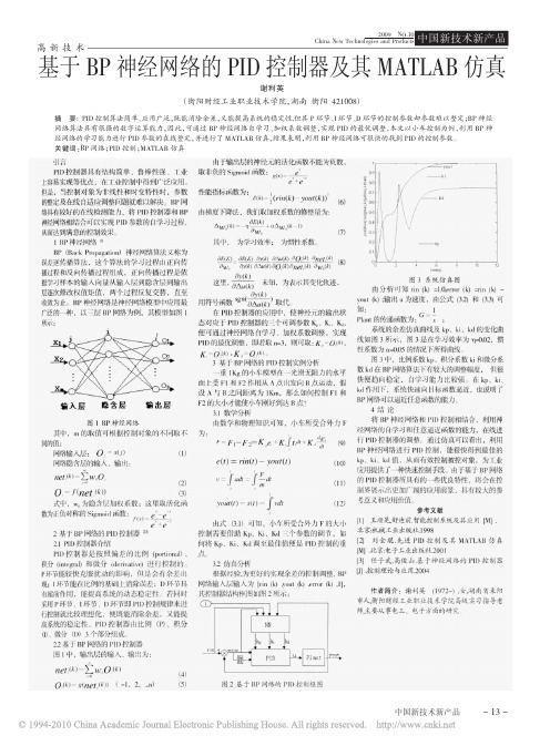
摘 要: PID 控制算法简单、应用广泛,既能消除余差,又能提高系统的稳定性,但其 P 环节、I 环节、D 环节的控制参数却参数难以整定;BP 神经 网络算法具有很强的数字运算能力,因此,可通过 BP 神经网络自学习、加权系数调整,实现 PID 的最优调整,本文以小车控制为例,利用 BP 神 经网络的学习能力进行 PID 参数的在线整定,并进行了 MATLAB 仿真,结果表明,利用 BP 神经网络可很快的找到 PID 的控制参数。 关键词:BP 网络;PID 控制;MATLAB 仿真
行 PID 控制器的调整。通过仿真可以看出,利用
BP 神经网络进行 PID 控制,能很快得到最佳的
kp、ki、kd 值,从而有效控制被控对象,为工业
应用提供了一种快速控制手段。由于基于 BP 网络
基于神经网络的PID自整定实验及其源程序
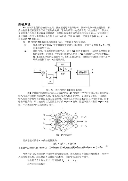
实验原理PID控制要取得较好的控制效果,就必须通过调整好比例、积分和微分三种控制作用,形成控制量中既相互配合又相互制约的关系,这种关系不一定是简单的“线性组合”,从变化无穷的非线性组合中可以找到最佳的。
神经网络所具有的任意非线性表达能力,可以通过对系统性能的学习来实现具有最佳组合的PID控制。
采用BP网络,可以建立参数Kp,Ki,Kd自学习的PID控制器。
基于BP网络的PID控制系统如图1所示,控制器由两部分构成:(1)经典的PID控制器,直接对被控对象进行闭环控制,并且三个参数Kp,Ki,Kd 为在线调整方式。
(2)神经网络,根据系统的运行状态,调节PID控制器的参数,以达到某种性能指标的最优化,使输出层神经元的输出状态对应于PID控制器的三个可调参数Kp,Ki,Kd通过神经网络的自学习、加权系数的调整,使神经网络输出对应于某种最优控制律下的PID控制器参数。
图1 基于神经网络的PID控制器结构图1中神经网络采用结构为三层的BP网络。
BP网络是一种单向传播的多层前向网络。
输入节点对应系统的运行状态量,如系统的偏差与偏差变化率,必要时要进行归一化处理。
输入变量的个数取决于被控系统的复杂程度;输出节点对应的是PID的三个可调参数。
由于输出不能为负,所以输出层活化函数取非负的Sigmoid函数,隐层取正负对称的Sigmoid函数。
本系统取BP网络的如图2所示。
图2 BP网络结构经典增量式数字PID的控制算法为:(1)网络的学习过程由正向和反向传播两部分组成。
如果输出层不能得到期望输出,那么转入反向传播过程,通过修改各层神经元的权值,使得输出误差信号最小。
输出层节点分别对应三个可调参数、、。
取性能指标函数为:按照梯度下降法修正网络的权系数,即按E(k)对加权系数的负梯度方向搜索调整,并附加一使快速收敛全局极小的惯性项式中,η为学习速率;α为惯性系数。
又基于BP 网络的PID 控制器控制算法如下:(1) 确定BP 网络的结构,即确定输入层节点数M 和隐含层节点数Q ,并给出各层加权系数的初值W 1ij(0)和W 2li(0),选定学校数率η和惯性系数α,此时K=1;(2) 采样得到rin(k)和yout(k),计算该时刻误差error(k)=rin(k)-yout(k); (3) 计算神经网络NN 各层神经元的输入、输出,NN 输出层的输出即为PID 控制器的三个可调参数Kp ,Ki ,Kd ;(4) 根据式()计算PID 控制器的输出u(k); (5) 进行神经网络学习,在线调整加权系数W 1ij(k)和W 2li(k),实现PID 控制参数的自适应调整;(6) 置k=k+1,返回(1)。
MATLAB程序代码--BP神经网络的设计实例
MATLAB程序代码-—BP神经网络的设计实例例1 采用动量梯度下降算法训练BP 网络。
训练样本定义如下:输入矢量为p =[—1 -2 3 1-1 1 5 —3]目标矢量为t = [-1 —1 1 1]解:本例的MA TLAB 程序如下:close allclearecho onclc% NEWFF--生成一个新的前向神经网络% TRAIN——对BP 神经网络进行训练% SIM—-对BP 神经网络进行仿真pause% 敲任意键开始clc% 定义训练样本% P 为输入矢量P=[-1,—2,3,1; -1, 1,5, -3];% T 为目标矢量T=[-1,—1,1,1];pause;clc%创建一个新的前向神经网络net=newff(minmax(P),[3,1],{'tansig’,'purelin'},'traingdm')%当前输入层权值和阈值inputWeights=net。
IW{1,1}inputbias=net.b{1}% 当前网络层权值和阈值layerWeights=net。
LW{2,1}layerbias=net。
b{2}pauseclc% 设置训练参数net.trainParam.show = 50;net.trainParam。
lr = 0.05;net。
trainParam.mc = 0。
9;net。
trainParam.epochs = 1000;net.trainParam。
goal = 1e—3;pauseclc%调用TRAINGDM 算法训练BP 网络[net,tr]=train(net,P,T);pauseclc%对BP 网络进行仿真A = sim(net,P)% 计算仿真误差E = T — AMSE=mse(E)pauseclcecho off例2 采用贝叶斯正则化算法提高BP 网络的推广能力。
在本例中,我们采用两种训练方法,即L—M 优化算法(trainlm)和贝叶斯正则化算法(trainbr),用以训练BP 网络,使其能够拟合某一附加有白噪声的正弦样本数据。
(完整版)BP神经网络matlab实例(简单而经典)
p=p1';t=t1';[pn,minp,maxp,tn,mint,maxt]=premnmx(p,t); %原始数据归一化net=newff(minmax(pn),[5,1],{'tansig','purelin'},'traingdx');%设置网络,建立相应的BP网络net.trainParam.show=2000; % 训练网络net.trainParam.lr=0.01;net.trainParam.epochs=100000;net.trainParam.goal=1e-5;[net,tr]=train(net ,pn,tn); %调用TRAINGDM算法训练BP 网络pnew=pnew1';pnewn=tramnmx(pnew,minp,maxp);anewn=sim(net,pnewn); %对BP网络进行仿真anew=postmnmx(anewn,mint,maxt); %还原数据y=anew';1、BP网络构建(1)生成BP网络=net newff PR S S SNl TF TF TFNl BTF BLF PF(,[1 2...],{ 1 2...},,,)PR:由R维的输入样本最小最大值构成的2R⨯维矩阵。
S S SNl:各层的神经元个数。
[ 1 2...]{ 1 2...}TF TF TFNl:各层的神经元传递函数。
BTF:训练用函数的名称。
(2)网络训练[,,,,,] (,,,,,,)=net tr Y E Pf Af train net P T Pi Ai VV TV(3)网络仿真=[,,,,] (,,,,)Y Pf Af E perf sim net P Pi Ai T{'tansig','purelin'},'trainrp'2、BP网络举例举例1、%traingdclear;clc;P=[-1 -1 2 2 4;0 5 0 5 7];T=[-1 -1 1 1 -1];%利用minmax函数求输入样本范围net = newff(minmax(P),T,[5,1],{'tansig','purelin'},'trainrp');net.trainParam.show=50;%net.trainParam.lr=0.05;net.trainParam.epochs=300;net.trainParam.goal=1e-5;[net,tr]=train(net,P,T);net.iw{1,1}%隐层权值net.b{1}%隐层阈值net.lw{2,1}%输出层权值net.b{2}%输出层阈值sim(net,P)举例2、利用三层BP神经网络来完成非线性函数的逼近任务,其中隐层神经元个数为五个。
bp神经网络matlab实例(bp神经网络matlab实例)

bp神经网络matlab实例(bp神经网络matlab实例)Case 1 training BP network by momentum gradient descent algorithm.Training samples are defined as follows:Input vector asP =[-1 -2 31-1 15 -3]The target vector is t = [-1 -1 1 1]Solution: the MATLAB program of this example is as follows:Close allClearEcho onCLC% NEWFF - generating a new feedforward neural network% TRAIN -- training BP neural network% SIM -- Simulation of BP neural networkPauseStart by hitting any keyCLCPercent defines training samples% P as input vectorP=[-1, -2, 3, 1; -1, 1, 5, -3];% T is the target vectorT=[-1, -1, 1, 1];Pause;CLC% create a new feedforward neural networkNet=newff (minmax (P), [3,1],{'tansig','purelin'},'traingdm')The current input layer weights and thresholds InputWeights=net.IW{1,1}Inputbias=net.b{1}The current network layer weights and thresholdsLayerWeights=net.LW{2,1}Layerbias=net.b{2}PauseCLC% set training parametersNet.trainParam.show = 50;Net.trainParam.lr = 0.05;Net.trainParam.mc = 0.9;Net.trainParam.epochs = 1000;Net.trainParam.goal = 1e-3;PauseCLC% call TRAINGDM algorithm to train BP network [net, tr]=train (net, P, T);PauseCLCSimulation of BP network by%A = sim (net, P)Calculate the simulation errorE = T - AMSE=mse (E)PauseCLCEcho offExample 2 adopts Bayesian regularization algorithm to improve the generalization ability of BP network. In this case, we used two kinds of training methods, namely L-M algorithm (trainlm) and the Bias regularization algorithm (trainbr), is used to train the BP network, so that it can fit attached to a white noise sine sample data. Among them, the sample data can be generated as follows MATLAB statements:Input vector: P = [-1:0.05:1];Target vector: randn ('seed', 78341223);T = sin (2*pi*P) +0.1*randn (size (P));Solution: the MATLAB program of this example is as follows: Close allClearEcho onCLC% NEWFF - generating a new feedforward neural network% TRAIN -- training BP neural network% SIM -- Simulation of BP neural networkPauseStart by hitting any keyCLC% define training sample vector% P as input vectorP = [-1:0.05:1];% T is the target vectorRandn ('seed', 78341223); T = sin (2*pi*P) +0.1*randn (size (P));Draw the sample data pointsPlot (P, T, +);Echo offHold on;Plot (P, sin (2*pi*P), ':');Draw sine curves without noiseEcho onCLCPauseCLC% create a new feedforward neural networkNet=newff (minmax (P), [20,1], {'tansig','purelin'});PauseCLCEcho offCLCDisp ('1. L-M optimization algorithm TRAINLM'); disp ('2. Bayesian regularization algorithm TRAINBR');Choice=input (\ "please select training algorithm (1,2): ');Figure (GCF);If (choice==1)Echo onCLC% using L-M optimization algorithm TRAINLMNet.trainFcn='trainlm';PauseCLC% set training parametersnet.trainparam.epochs = 500;net.trainparam.goal = 1e-6;NET(.NET);%重新初始化暂停中图分类号“(选择= = 2)回声中图分类号%采用贝叶斯正则化算法trainbr trainfcn = 'trainbr”网;暂停中图分类号%设置训练参数net.trainparam.epochs = 500;randn(“种子”,192736547);NET(.NET);%重新初始化暂停中图分类号结束调用相应算法训练BP网络% [净额],列车=(净额,P,T);暂停中图分类号对BP网络进行仿真%a = sim(NET,p);%计算仿真误差e = a;MSE=MSE(e)暂停中图分类号%绘制匹配结果曲线关闭所有;图(p,a,p,t,+,p,p,p(2),“,”;暂停;中图分类号回音通过采用两种不同的训练算法,我们可以得到如图1和图2所示的两种拟合结果。
- 1、下载文档前请自行甄别文档内容的完整性,平台不提供额外的编辑、内容补充、找答案等附加服务。
- 2、"仅部分预览"的文档,不可在线预览部分如存在完整性等问题,可反馈申请退款(可完整预览的文档不适用该条件!)。
- 3、如文档侵犯您的权益,请联系客服反馈,我们会尽快为您处理(人工客服工作时间:9:00-18:30)。
BP神经网络整定的PID控制算法matlab源程序,系统为二阶闭环系统。
%BP based PID Control
clear all;
close all;
xite=0.28;
alfa=0.001;
IN=4;H=5;Out=3; %NN Structure
wi=0.50*rands(H,IN);
wi_1=wi;wi_2=wi;wi_3=wi;
wo=0.50*rands(Out,H);
wo_1=wo;wo_2=wo;wo_3=wo;
x=[0,0,0];
u_1=0;u_2=0;u_3=0;u_4=0;u_5=0;
y_1=0;y_2=0;y_3=0;
Oh=zeros(H,1); %Output from NN middle layer
I=Oh; %Input to NN middle layer
error_2=0;
error_1=0;
ts=0.01;
sys=tf(2.6126,[1,3.201,2.7225]); %建立被控对象传递函数
dsys=c2d(sys,ts,'z'); %把传递函数离散化
[num,den]=tfdata(dsys,'v'); %离散化后提取分子、分母
for k=1:1:2000
time(k)=k*ts;
rin(k)=40;
yout(k)=-den(2)*y_1-den(3)*y_2+num(2)*u_2+num(3)*u_3;
error(k)=rin(k)-yout(k);
xi=[rin(k),yout(k),error(k),1];
x(1)=error(k)-error_1;
x(2)=error(k);
x(3)=error(k)-2*error_1+error_2;
epid=[x(1);x(2);x(3)];
I=xi*wi';
for j=1:1:H
Oh(j)=(exp(I(j))-exp(-I(j)))/(exp(I(j))+exp(-I(j))); %Middle Layer end
K=wo*Oh; %Output Layer
for l=1:1:Out
K(l)=exp(K(l))/(exp(K(l))+exp(-K(l))); %Getting kp,ki,kd end
kp(k)=K(1);ki(k)=K(2);kd(k)=K(3);
Kpid=[kp(k),ki(k),kd(k)];
du(k)=Kpid*epid;
u(k)=u_1+du(k);
if u(k)>=45 % Restricting the output of controller u(k)=45;
end
if u(k)<=-45
u(k)=-45;
end
dyu(k)=sign((yout(k)-y_1)/(u(k)-u_1+0.0000001));
%Output layer
for j=1:1:Out
dK(j)=2/(exp(K(j))+exp(-K(j)))^2;
end
for l=1:1:Out
delta3(l)=error(k)*dyu(k)*epid(l)*dK(l);
end
for l=1:1:Out
for i=1:1:H
d_wo=xite*delta3(l)*Oh(i)+alfa*(wo_1-wo_2);
end
end
wo=wo_1+d_wo+alfa*(wo_1-wo_2);
%Hidden layer
for i=1:1:H
dO(i)=4/(exp(I(i))+exp(-I(i)))^2;
end
segma=delta3*wo;
for i=1:1:H
delta2(i)=dO(i)*segma(i);
end
d_wi=xite*delta2'*xi;
wi=wi_1+d_wi+alfa*(wi_1-wi_2);
%Parameters Update
u_5=u_4;u_4=u_3;u_3=u_2;u_2=u_1;u_1=u(k); y_2=y_1;y_1=yout(k);
wo_3=wo_2;
wo_2=wo_1;
wo_1=wo;
wi_3=wi_2;
wi_2=wi_1;
wi_1=wi;
error_2=error_1;
error_1=error(k);
end
figure(1);
plot(time,rin,'r',time,yout,'b');
xlabel('time(s)');ylabel('rin,yout');
figure(2);
plot(time,error,'r');
xlabel('time(s)');ylabel('error');
figure(3);
plot(time,u,'r');
xlabel('time(s)');ylabel('u');
figure(4);
subplot(311);
plot(time,kp,'r');
xlabel('time(s)');ylabel('kp');
subplot(312);
plot(time,ki,'g');
xlabel('time(s)');ylabel('ki');
subplot(313);
plot(time,kd,'b');
xlabel('time(s)');ylabel('kd');。