数学建模与系统仿真网课答案.docx
系统建模与仿真习题2及答案

系统建模与仿真习题二及答案1. 考虑如图所示的典型反馈控制系统框图(1)假设各个子传递函数模型为66.031.05.02)(232++-+=s s s s s G ,s s s G c 610)(+=,21)(+=s s H 分别用feedback ()函数以及G*Gc/(1+G*Gc*H)(要最小实现)方法求该系统的传递函数模型。
(2) 假设系统的受控对象模型为s e s s s G 23)1(12)(-+=,控制器模型为 ss s G c 32)(+=,并假设系统是单位负反馈,分别用feedback ()函数以及G*Gc/(1+G*Gc*H)(要最小实现)方法能求出该系统的传递函数模型?如果不能,请近似该模型。
解:(1)clc;clear;G=tf([2 0 0.5],[1 -0.1 3 0.66]);Gc=tf([10 6],[1 0]);H=tf(1,[1 2]);G1=feedback(G*Gc,H)G2=G*Gc/(1+G*Gc*H)Gmin=minreal(G2)结果:Transfer function:20 s^4 + 52 s^3 + 29 s^2 + 13 s + 6s^5 + 1.9 s^4 + 22.8 s^3 + 18.66 s^2 + 6.32 s + 3Transfer function:20 s^8 + 50 s^7 + 83.8 s^6 + 179.3 s^5 + 126 s^4 + 57.54 s^3 + 26.58 s^2 + 3.96 ss^9 + 1.8 s^8 + 25.61 s^7 + 22.74 s^6 + 74.11 s^5 + 73.4 s^4 + 30.98 s^3+ 13.17 s^2 + 1.98 s Transfer function:20 s^4 + 52 s^3 + 29 s^2 + 13 s + 6s^5 + 1.9 s^4 + 22.8 s^3 + 18.66 s^2 + 6.32 s + 3(2)由于s c e s s s s G s G 232)1(3624)(*)(-++= 方法1:将s e 2-转换为近似多项式。
系统建模与仿真_考题答案

共10题 每题10分1、什么是数学建模形式化的表示?试列举一例说明形式化表示与非形式化表示的区别;模型的非形式描述是说明实际系统的本质,但不是详尽描述。
是对模型进行深入研究的基础。
主要由模型的实体、包括参变量的描述变量、实体间的相互关系及有必要阐述的假设组成。
模型的非形式描述主要说明实体、描述变量、实体间的相互关系及假设等。
例子:环形罗宾服务模型的非形式描述:实体CPU ,USR1,…,USR5描述变量CPU:Who,Now(现在是谁)----范围{1,2,…,5}; Who.Now=i 表示USRi 由CPU 服务。
USR :Completion.State (完成情况)----范围[0,1];它表示USR 完成整个程序任务的比例。
参变量i X -----范围[0,1];它表示USRi 每次完成程序的比率。
实体相互关系(1)CPU 以固定速度依次为用户服务,即Who.Now 为1,2,3,4,5,1,2…..循环运行。
(2)当Who.Now=I,CPU 完成USRi 余下的i X 工作。
假设:CPU 对USR 的服务时间固定,不依赖于USR 的程序;USRi 的进程是由各自的参变量i X 决定。
2、模型描述变量化简的四种方法比较;建模过程中,在能满足建模的前提下,系统的描述变量应是愈简单愈好。
模型描述变量一般有以下四种方法:(1)、淘汰一个或多个实体、描述变量或相互关系规则;建模者决定淘汰那些次要因素,只要忽略的因素不会显著地改变整个模型行为,相反却使不必要的复杂了。
淘汰一个实体可能要淘汰或修改其他实体:淘汰一个实体,需要淘汰所有涉及这个实体的描述变量;淘汰一个描述变量,需要淘汰或修改涉及该变量的相互关系。
(2)、随机变量取代确定性变量;在一个确定性模型中,相互关系的规则控制着整个描述变量的值。
有些随机值也是由相互关系的规则确定,为了使模型相对简化,可利用概率原理,用随机变量来取代某些变量的相互关系规则,从而将影响变量转换成随机变量。
数学建模答案(完整版)
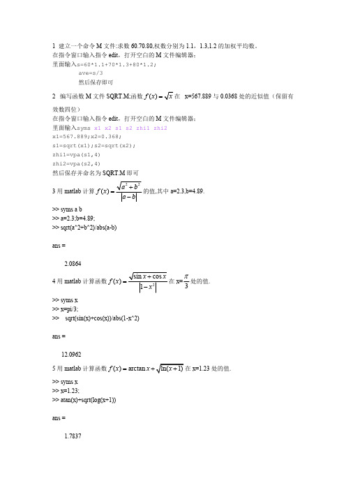
1 建立一个命令M 文件:求数60.70.80,权数分别为1.1,1.3,1.2的加权平均数。
在指令窗口输入指令edit ,打开空白的M 文件编辑器;里面输入s=60*1.1+70*1.3+80*1.2;ave=s/3然后保存即可2 编写函数M 文件SQRT.M;函数 x=567.889与0.0368处的近似值(保留有()f x =效数四位)在指令窗口输入指令edit ,打开空白的M 文件编辑器;里面输入syms x1 x2 s1 s2 zhi1 zhi2 x1=567.889;x2=0.368;s1=sqrt(x1);s2=sqrt(x2);zhi1=vpa(s1,4)zhi2=vpa(s2,4)然后保存并命名为SQRT.M 即可3用matlab 计算的值,其中a=2.3,b=4.89.()f x >> syms a b >> a=2.3;b=4.89;>> sqrt(a^2+b^2)/abs(a-b)ans = 2.08644用matlab 计算函数在x=处的值.()f x =3π>> syms x >> x=pi/3;>> sqrt(sin(x)+cos(x))/abs(1-x^2)ans = 12.09625用matlab 计算函数在x=1.23处的值.()arctan f x x =+>> syms x >> x=1.23;>> atan(x)+sqrt(log(x+1))ans = 1.78376 用matlab 计算函数在x=-2.1处的值.()()f x f x ==>> syms x >> x=-2.1;>> 2-3^x*log(abs(x))ans =1.92617 用蓝色.点连线.叉号绘制函数在[0,2]上步长为0.1的图像.>> syms x y>> x=0:0.2:2;y=2*sqrt(x);>> plot(x,y,'b.-')8 用紫色.叉号.实连线绘制函数在上步长为0.2的图像.ln 10y x =+[20,15]-->> syms x y>> x=-20:0.2:-15;y=log(abs(x+10));>> plot(x,y,'mx-')ln 10[20,y x =+--9 用红色.加号连线 虚线绘制函数在[-10,10]上步长为0.2的图像.sin(22x y π=->> syms x y;>> x=-10:0.2:10;y=sin(x/2-pi/2);>> plot(x,y,'r+--')10用紫红色.圆圈.点连线绘制函数在上步长为0.2的图像.sin(2)3y x π=+[0,4]πsin(2)sin()[0,4]322x y x y πππ=+=->> syms x y >> x=0:0.2:4*pi;y=sin(2*x+pi/3);>> plot(x,y,'mo-.')11 在同一坐标中,用分别青色.叉号.实连线与红色.星色.虚连线绘制y=与.y =>> syms x y1 y2>> x=0:pi/50:2*pi;y1=cos(3*sqrt(x));y2=3*cos(sqrt(x));>> plot(x,y1,'cx-',x,y2,'r*--')12 在同一坐标系中绘制函数这三条曲线的图标,并要求用两种方法加234,,y x y x y x ===各种标注.234,,y x y x y x ===>> syms x y1 y2 y3;>> x=-2:0.1:2;y1=x.^2;y2=x.^3;y3=x.^4;plot(x,y1,x,y2,x,y3);13 作曲线的3维图像2sin x t y t z t ⎧=⎪=⎨⎪=⎩>> syms x y t z >> t=0:1/50:2*pi;>> x=t.^2;y=sin(t);z=t;>> stem3(x,y,z)14 作环面在上的3维图像(1cos )cos (1cos )sin sin x u v y u v z u =+⎧⎪=+⎨⎪=⎩(0,2)(0,2)ππ⨯>> syms x y u v z>> u=0:pi/50:2*pi;v=0:pi/50:2*pi;>>x=(1+cos(u)).*cos(v);y=(1+cos(u)).*sin(v);z=sin(u);>> plot3(x,y,z)15 求极限0lim x +→0lim x +→>> syms x y >> y=sin(2^0.5*x)/sqrt(1-cos(x));>> limit(y,x,0,'right') ans = 216 求极限1201lim (3x x +→>> syms y x >> y=(1/3)^(1/(2*x));>> limit(y,x,0,'right') ans = 017求极限lim x >> syms x y >> y=(x*cos(x))/sqrt(1+x^3);>> limit(y,x,+inf) ans = 018 求极限21lim (1x x x x →+∞+->> syms x y >> y=((x+1)/(x-1))^(2*x);>> limit(y,x,+inf) ans = exp(4)19 求极限01cos 2lim sin x xx x →->> syms x y >> y=(1-cos(2*x))/(x*sin(x));>> limit(y,x,0) ans = 220 求极限 x →>> syms x y >> y=(sqrt(1+x)-sqrt(1-x))/x;>> limit(y,x,0) ans = 121 求极限2221lim 2x x x x x →+∞++-+>> syms x y >> y=(x^2+2*x+1)/(x^2-x+2);>> limit(y,x,+inf) ans = 122 求函数y=的导数5(21)arctan x x -+>> syms x y >> y=(2*x-1)^5+atan(x);>> diff(y) ans = 10*(2*x - 1)^4 + 1/(x^2 + 1)23 求函数y=的导数2tan 1x x y x=+>> syms y x>> y=(x*tan(x))/(1+x^2);>> diff(y)ans =tan(x)/(x^2 + 1) + (x*(tan(x)^2 + 1))/(x^2 + 1) - (2*x^2*tan(x))/(x^2 + 1)^224 求函数的导数3tan x y e x -=>> syms y x >> y=exp^(-3*x)*tan(x)>> y=exp(-3*x)*tan(x) y = exp(-3*x)*tan(x) >> diff(y) ans = exp(-3*x)*(tan(x)^2 + 1) - 3*exp(-3*x)*tan(x)25 求函数y=在x=1的导数22ln sin 2x x π+>> syms x y >> y=(1-x)/(1+x);>> diff(y,x,2) ans = 2/(x + 1)^2 - (2*(x - 1))/(x + 1)^3 >> syms x y >> y=2*log(x)+sin(pi*x/2)^2;>> dxdy=diff(y) dxdy = 2/x + pi*cos((pi*x)/2)*sin((pi*x)/2)zhi=subs(dxdy,1)zhi = 226 求函数y=的二阶导数01cos 2lim sin x x x x →-11x x-+>> syms x y>> y=(1-x)/(1+x);>> diff(y,x,2) ans = 2/(x + 1)^2 - (2*(x - 1))/(x + 1)^327 求函数的导数;>> syms x y >> y=((x-1)^3*(3+2*x)^2/(1+x)^4)^0.2;>> diff(y) ans = (((8*x + 12)*(x - 1)^3)/(x + 1)^4 + (3*(2*x + 3)^2*(x - 1)^2)/(x + 1)^4 - (4*(2*x + 3)^2*(x - 1)^3)/(x + 1)^5)/(5*(((2*x + 3)^2*(x - 1)^3)/(x + 1)^4)^(4/5))28在区间()内求函数的最值.,-∞+∞43()341f x x x =-+>> f='-3*x^4+4*x^3-1';>> [x,y]=fminbnd(f,-inf,inf)x =NaN y = NaN >> f='3*x^4-4*x^3+1';>> [x,y]=fminbnd(f,-inf,inf)x = NaN y = NaN29在区间(-1,5)内求函数发的最值.()(f x x =->> f='(x-1)*x^0.6';>> [x,y]=fminbnd(f,-1,5)x =0.3750y = -0.3470>> >> f='-(x-1)*x^0.6';>> [x,y]=fminbnd(f,-1,5)x = 4.9999y = -10.505930 求不定积分(ln 32sin )x x dx -⎰(ln 32sin )x x dx -⎰>> syms x y >> y=log(3*x)-2*sin(x);>> int(y) ans = 2*cos(x) - x + x*log(3) + x*log(x)31求不定积分2sin x e xdx ⎰>> syms x y>> y=exp(x)*sin(x)^2;>> int(y)ans =-(exp(x)*(cos(2*x) + 2*sin(2*x) - 5))/1032. 求不定积分 >> syms x y >> y=x*atan(x)/(1+x)^0.5;>> int(y)Warning: Explicit integral could not be found. ans = int((x*atan(x))/(x + 1)^(1/2), x)33.计算不定积分2(2cos )x x x e dx --⎰>> syms x y >> y=1/exp(x^2)*(2*x-cos(x));>> int(y)Warning: Explicit integral could not be found. ans = int(exp(-x^2)*(2*x - cos(x)), x)34.计算定积分10(32)xe x dx -+⎰>> syms x y >> y=exp(-x)*(3*x+2);>> int(y,0,1) ans = 5 - 8*exp(-1)10(32)x e x dx -+⎰35.计算定积分0x →120(1)cos x arc xdx+⎰>> syms y x>> y=(x^2+1)*acos(x);>> int(y,0,1)ans =11/936.计算定积分10cos ln(1)x x dx +⎰>> syms x y >> y=(cos(x)*log(x+1));>> int(y,0,1)Warning: Explicit integral could not be found. ans = int(log(x + 1)*cos(x), x == 0..1)37计算广义积分;2122x x dx +∞++-∞⎰>> syms y x >> y=(1/(x^2+2*x+2));>> int(y,-inf,inf) ans = pi 38.计算广义积分;20x dx x e +∞-⎰>> syms x y>> y=x^2*exp(-x);>> int(y,0,+inf)ans =2。
完整版系统仿真答案
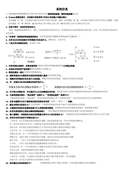
系统仿真1、连续数据和离散数据的直方图分别与理论分布的概率密度函数、概率质量函数相对应。
2、Flexsim建模过程中,如何建立和取消两个实体之间的输入和输出端口按住键盘“A”键,点击鼠标左键可以在两个实体之间连接一条线。
按住键盘“Q”键,点击鼠标左键可以在两个实体之间删除一条线按住键盘“S”“W”键同理。
AQ用在固定元件与固定元件之间,SW用在固定元件与可移动元件之间。
3、仿真中事件、活动和实体的定义。
实体:组成系统的物理单元。
事件:引起系统状态变化的行为,即系统的动态过程是靠事件来驱动的。
活动:两个相邻发生的事件之间的过程。
4、“仿真钟”的推进和推进速度的特点。
仿真钟的推进呈现跳跃性推进速度具有随机性。
?5、具有无记忆性的连续分布和离散分布各是什么。
指数分布、几何分布。
6、三角分布各参数的求法。
高度=2/(c-a)7、在研究排队系统时,决策者通常要在服务台利用率和顾客满意程度之间做出权衡。
8、舍选技术的效率严重依赖于将拒绝数最小化的能力。
9、模型的假设一般分结构假设和数据假设。
10、能够快速显示出模型的合理性的两组统计量是当前容量和总数。
11、预测区间和置信区间各是什么的度量。
预测区间是风险的度量,而置信区间是误差的度量。
12、单、多服务台队列达到稳定的条件是什么。
13、对于绝大多数队列,可以通过什么方式来缩短队列长度。
通过减小服务台利用率或服务时间波动的方式来缩短队列长度。
15、当系统容量有限时,“到达速率”是指什么,“有效到达速率”是指什么?当系统容量有限时,“到达速率”(单位时间的到达数目)和“有效到达速率”(单位时间内到达并进入系统的数目)16、仿真与建模可以用于解答现实世界系统各种各样“如果……就会……”问题。
17、输出分析的目的是什么?目的是预测一个系统的性能或比较两个或多个备选系统设计的性能。
18、本课程所讲述的仿真模型是属于什么类型的数学模型。
本课程所讲述的仿真模型是系统的一类特殊数学模型。
智慧树知到《数学建模与系统仿真》章节测试答案

智慧树知到《数学建模与系统仿真》章节测试答案第一章单元测试1.数学模型是根据特定对象和特定目的,做出必要假设,运用适当数学工具得到一个数学结构的理论表述。
答案:对2.数学建模是利用数学方法解决实际问题的一种实践。
通过抽象、简化、假设、引入变量等处理过程后,将实际问题用数学方式表达,建立起数学模型,然后运用先进的数学方法及计算机技术进行求解,是对实际问题的完全解答和真实反映,结果真实可靠。
答案:对3.数学模型是用数学符号、数学公式、程序、图、表等刻画客观事物的本质属性与内在联系的理想化表述。
数学建模就是建立数学模型的全过程(包括表述、求解、解释、检验)。
答案:对4.数学模型(Mathematical Model)强调的是过程;数学建模(Mathematical Modeling)强调的是结果。
答案:错5.人口增长的Logistic模型表明人口增长过程是先快后慢。
答案:对6.MATLAB的主要功能包括符号计算、绘图功能、与其他程序语言交互的接口和数值计算。
答案:符号计算、绘图功能、与其他程序语言交互的接口、数值计算7.Mathematica的基本功能包括语言功能(Programing Language)、符号运算(Algebric n)、数值运算(XXX)和图像处理(Graphics)。
答案:语言功能(Programing Language)、符号运算(Algebric n)、数值运算(Numeric n)、图像处理(Graphics)8.数值计算是Maple、MATLAB和Mathematica的主要功能之一。
答案:Maple、MATLAB、XXX9.评阅数学建模论文的标准包括表述的清晰性、建模的创造性和论文假设的合理性。
答案:表述的清晰性、建模的创造性、论文假设的合理性10.中国(全国)大学生数学建模竞赛(CUMCM)每年举办一次。
该竞赛开始于70年代初。
答案:一年举办一次,开始于70年代初。
10、微分方程模型可以用于描述物体动态变化过程,并且可以用来预测对象特征的未来状态。
系统建模与仿真习题3及答案
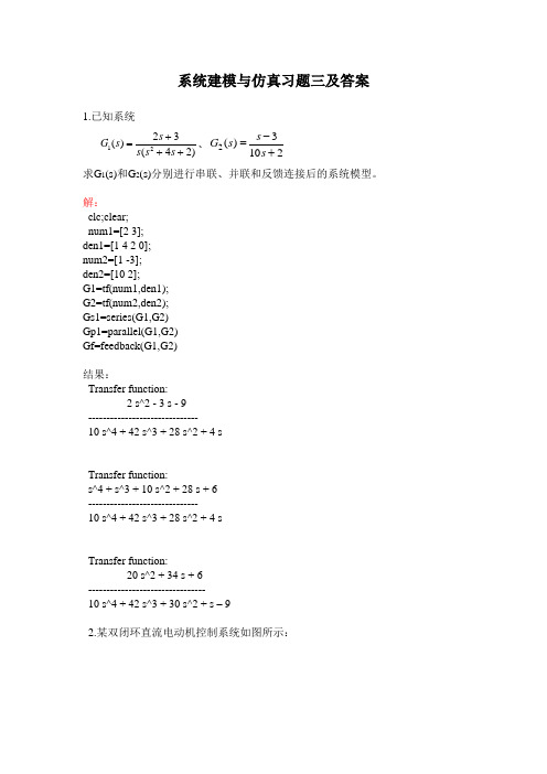
系统建模与仿真习题三及答案1.已知系统)24(32)(21+++=s s s s s G 、2103)(2+-=s s s G 求G 1(s)和G 2(s)分别进行串联、并联和反馈连接后的系统模型。
解:clc;clear;num1=[2 3];den1=[1 4 2 0];num2=[1 -3];den2=[10 2];G1=tf(num1,den1);G2=tf(num2,den2);Gs1=series(G1,G2)Gp1=parallel(G1,G2)Gf=feedback(G1,G2)结果:Transfer function:2 s^2 -3 s - 9------------------------------10 s^4 + 42 s^3 + 28 s^2 + 4 sTransfer function:s^4 + s^3 + 10 s^2 + 28 s + 6------------------------------10 s^4 + 42 s^3 + 28 s^2 + 4 sTransfer function:20 s^2 + 34 s + 6--------------------------------10 s^4 + 42 s^3 + 30 s^2 + s – 92.某双闭环直流电动机控制系统如图所示:利用feedback( )函数求系统的总模型。
解:模型等价为:编写程序:clc;clear;s=tf('s');G1=1/(0.01*s+1);G2=(0.17*s+1)/(0.085*s);G3=G1;G4=(0.15*s+1)/(0.051*s);G5=70/(0.0067*s+1);G6=0.21/(0.15*s+1);G7=(s+2)/s;G8=0.1*G1;G9=0.0044/(0.01*s+1);sys1=feedback(G6*G7,0.212);sys2=feedback(sys1*G4*G5,G8*inv(G7)); sys=G1*feedback(sys2*G2*G3,G9)结果:Transfer function:3.749e-005 s^6 + 0.008117 s^5 + 0.5024 s^4 + 6.911 s^3 + 36.57 s^2 + 78.79 s + 58.8 -------------------------------------------------------------------------------------------------------4.357e-014 s^10 + 2.432e-011 s^9 +5.43e-009 s^8 +6.303e-007 s^7 + 4.145e-005 s^6 + 0.001578 s^5 + 0.03217 s^4 + 0.2098 s^3 + 0.4116 s^2 + 0.3467 s + 0.2587根据需要可忽略高阶项。
数学建模 建模答案.docx

programi :(1) function [accum, varargout] = CircularHough_Grd(img, radrange, varargin) %Detect circular shapes in a grayscale image. Resolve their center %positions and radii.%% [accum, circen, cirrad, dbg_LMmask] = CircularHough_Grd(% img, radrange, grdthres, fltr4LM_R, multirad, fltr4accum)% Circular Hough transform based on the gradient field of an image.% NOTE: Operates on grayscale images, NOT B/W bitmaps.% NO loops in the implementation of Circular Hough transform,% which means faster operation but at the same time larger% memory consumption.%%%%%%%%% INPUT: (img, radrange, grdthres, fltr4LM_R, multirad, fltr4accum) % % img: A 2-D grayscale image (NO B/W bitmap)%% radrange: The possible minimum and maximum radii of the circles% to be searched, in the format of% [minimum radius , maximum_radius] (unit: pixels)% **NOTE**: A smaller range saves computational time and% memory.%% grdthres: (Optional, default is 10, must be non-negative)% The algorithm is based on the gradient field of the% input image. A thresholding on the gradient magnitude% is performed before the voting process of the Circular% Hough transform to remove the Uniform intensity'% (sort-of) image background from the voting process.% In other words, pixels with gradient magnitudes smaller% than 'grdthres' are NOT considered in the computation.% **NOTE**: The default parameter value is chosen for% images with a maximum intensity close to 255. For cases% with dramatically different maximum intensities, e.g.% 10-bit bitmaps in stead of the assumed 8-bit, the default% value can NOT be used. A value of 4% to 10% of the maximum% intensity may work for general cases.%% fltr4LM_R: (Optional, default is 8, minimum is 3)% The radius of the filter used in the search of local% maxima in the accumulation array. To detect circles whose% shapes are less perfect, the radius of the filter needs% to be set larger.%% multirad: (Optional, default is 0.5)% In case of concentric circles, multiple radii may be% detected corresponding to a single center position. This% argument sets the tolerance of picking up the likely% radii values. It ranges from 0.1 to 1, where 0.1% corresponds to the largest tolerance, meaning more radii % values will be detected, and 1 corresponds to the smallest % tolerance, in which case only the "principal" radius will% be picked up.%% fltr4accum: (Optional. A default filter will be used if not given)% Filter used to smooth the accumulation array. Depending % on the image and the parameter settings, the accumulation % array built has different noise level and noise pattern% (e.g. noise frequencies). The filter should be set to an% appropriately size such that ifs able to suppress the% dominant noise frequency.%%%%%%%%% OUTPUT: [accum, circen, cirrad, dbg_LMmask]%% accum: The result accumulation array from the Circular Hough% transform. The accumulation array has the same dimension % as the input image.%% circen: (Optional)% Center positions of the circles detected. Is a N-by-2% matrix with each row contains the (x, y) positions% of a circle. For concentric circles (with the same center% position), say k of them, the same center position will% appear k times in the matrix.%% cirrad: (Optional)% Estimated radii of the circles detected. Is a N-by-1% column vector with a one-to-one correspondance to the% output tircen*. A value 0 for the radius indicates a% failed detection of the circle's radius.%% dbg_LMmask: (Optional, for debugging purpose)% Mask from the search of local maxima in the accumulation % array.%%%%%%%%%% EXAMPLE #0:% rawimg = imread('TestImg_CHT_a2.bmp');% tic;% [accum, circen, cirrad] = CircularHough_Grd(rawimg, [15 60]);% toe;% figure(l); imagesc(accum); axis image;% title(,Accumulation Array from Circular Hough Transfbrm,);% figure(2); imagesc(rawimg); colormap(,gray,); axis image;% hold on;% plot(circen(:,l), circen(:,2), *r+');% for k = 1 : size(circen, 1),% DrawCircle(circen(k, 1), circen(k,2), cirrad(k), 32,,b」);% end% hold off;% title([*Raw Image with Circles Detected% '(center positions and radii marked)*]);% figure(3); surf(accum, 'EdgeColoF, hone'); axis ij;% title('3-D View of the Accumulation Array*);%% COMMENTS ON EXAMPLE #0:% Kind of an easy case to handle. To detect circles in the image whose% radii range from 15 to 60. Default values for arguments 'grdthres',% 'fltr4LM_R', 'multirad* and ,fltr4accum, are used.%%%%%%%%%% EXAMPLE #1:% rawimg = imread('TestImg_CHT_a3.bmp');% tic;% [accum, circen, cirrad] = CircularHough_Grd(rawimg, [15 60], 10, 20);% toe;% figure(l); imagesc(accum); axis image;% title(,Accumulation Array from Circular Hough Transfbrm,);% figure(2); imagesc(rawimg); colormap('gray'); axis image;% hold on;% plot(circen(:,l), circen(:,2), T+');% for k = 1 : size(circen, 1),% DrawCircle(circen(k, 1), circen(k,2), cirrad(k), 32, 'b-');% end% hold off;% title([*Raw Image with Circles Detected% '(center positions and radii marked)*]);% figure(3); surf(accum, 'EdgeColoF, hone'); axis ij;% title(*3-D View of the Accumulation Array*);%% COMMENTS ON EXAMPLE #1:% The shapes in the raw image are not very good circles. As a result,% the profile of the peaks in the accumulation array are kind of% 'stumpy', which can be seen clearly from the 3-D view of the% accumulation array, (As a comparison, please see the sharp peaks in % the accumulation array in example #0) To extract the peak positions % nicely, a value of 20 (default is 8) is used for argument 'fltr4LM_R', % which is the radius of the filter used in the search of peaks.%%%%%%%%%% EXAMPLE #2:% rawimg = imread(,TestImg_CHT_b3 .bmp1);% fltr4img = [1 1 1 1 1; 1 2 2 2 1; 1 2 4 2 1; 1 2 2 2 1; 1 1 1 1 1];% fltr4img = fltr4img / sum(fltr4img(:));% imgfltrd = filter2( fltr4img , rawimg );% tic;% [accum, circen, cirrad] = CircularHough_Grd(imgfltrd, [15 80], 8, 10); % toe;% figure(l); imagesc(accum); axis image;% title(,Accumulation Array from Circular Hough Transfbrm,);% figure(2); imagesc(rawimg); colormap('gray'); axis image;% hold on;% plot(circen(:,l), circen(:,2), T+');% for k = 1 : size(circen, 1),% DrawCircle(circen(k, 1), circen(k,2), cirrad(k), 32, 'b-');% end% hold off;% title([*Raw Image with Circles Detected% '(center positions and radii marked)*]);%% COMMENTS ON EXAMPLE #2:% The circles in the raw image have small scale irregularities along % the edges, which could lead to an accumulation array that is bad for % local maxima detection. A 5-by-5 filter is used to smooth out the % small scale irregularities. A blurred image is actually good for the % algorithm implemented here which is based on the image's gradient % field.%%%%%%%%%% EXAMPLE #3:% rawimg = imread('TestImg_CHT_c3.bmp');% fltr4img = [1 1 1 1 1; 1 2 2 2 1; 1 2 4 2 1; 1 2 2 2 1; 1 1 1 1 1];% fltr4img = fltr4img / sum(fltr4img(:));% imgfltrd = filter2( fltr4img , rawimg );% tic;% [accum, circen, cirrad]=...% CircularHough_Grd(imgfltrd, [15 105], 8, 10, 0.7);% toe;% figure(l); imagesc(accum); axis image;% figure(2); imagesc(rawimg); colormap(,gray,); axis image;% hold on;% plot(circen(:,l), circen(:,2), *r+');% for k = 1 : size(circen, 1),% DrawCircle(circen(k, 1), circen(k,2), cirrad(k), 32,,b」);% end% hold off;% title([*Raw Image with Circles Detected% '(center positions and radii marked)*]);%% COMMENTS ON EXAMPLE #3:% Similar to example #2, a filtering before circle detection works for% noisy image too. 'multirad* is set to 0.7 to eliminate the false% detections of the circles* radii.%%%%%%%%%% BUG REPORT:% This is a beta version. Please send your bug reports, comments and% suggestions to pengtao@ . Thanks.%%%%%%%%%%% INTERNAL PARAMETERS:% The INPUT arguments are just part of the parameters that are used by% the circle detection algorithm implemented here. Variables in the code% with a prefix ,prm_, in the name are the parameters that control the% judging criteria and the behavior of the algorithm. Default values for% these parameters can hardly work for all circumstances. Therefore, at% occasions, the values of these INTERNAL PARAMETERS (parameters that% are NOT exposed as input arguments) need to be fine-tuned to make% the circle detection work as expected.% The following example shows how changing an internal parameter could% influence the detection result.% 1. Change the value of the internal parameter 'prm LM LoBndRa* to 0.4% (default is 0.2)% 2. Run the following matlab code:% fltr4accum = [1 2 1; 2 6 2; 1 2 1];% fltr4accum = fltr4accum / sum(fltr4accum(:));% rawimg = imread(,Frame_0_0022jportion.jpg,);% tic;% [accum, circen] = CircularHough_Grd(rawimg,...% [4 14], 10, 4, 0.5, fltr4accum);% toe;% figure(l); imagesc(accum); axis image;% title(*Accumulation Array from Circular Hough Transform*);% figure(2); imagesc(rawimg); colormap(,gray,); axis image;% hold on; plot(circen(:,l), circen(:,2), "); hold off;% title('Raw Image with Circles Detected (center positions marked)*);% 3. See how different values of the parameter 'prm LM LoBndRa* could % influence the result.% Author: Tao Peng% Department of Mechanical Engineering% University of Maryland, College Park, Maryland 20742, USA% pengtao@% Version: Beta Revision: Mar. 07, 2007%%%%%%%% Arguments and parameters %%%%%%%%%%%%%%%%%%%%%%%%%%%%%%%%%%%% Validation of argumentsif ndims(img)〜=2 || 〜isnumeric(img),error(*CircularHough_Grd: "img" has to be 2 dimensionaf);endif 〜all(size(img) >= 32),erro^'CircularHough Grd: "img" has to be larger than 32-by-32');endif numel(radrange)〜=2 || -isnumeric(radrange),error([*CircularHough_Grd: "radrange" has to be \ ...'a two-element vector1]);endprm_r_range = sort(max( [0,0;radrange( 1 ),radrange(2)]));% Parameters (default values)prmgrdthres = 10;prmfltrLMR = 8;prmmultirad = 0.5;funccompucen = true;funccompuradii = true;% Validation of argumentsvapgrdthres = 1;if nargin > (1 + vap_grdthres),if isnumeric(varargin{vap grdthres}) && ...varargin(vap grdthres} (1) >= 0,prm_grdthres = varargin {vapgrdthres} (1);elseerror(['CircularHough_Grd: "grdthres" has to be'a non-negative number1]);endendvap_fltr4LM = 2; % filter for the search of local maximaif nargin > (1 + vap_fltr4LM),if isnumeric(varargin{vap_fltr4LM}) && varargin{vap_fltr4LM}(1) >= 3, prmfltrLMR = varargin{vap_fltr4LM} (1);elseerror([,CircularHough_Grd: n fltr4LM_R n has to belarger than or equal to 3']);endendvap_multirad = 3;if nargin > (1 + vap multirad),if isnumeric(varargin{vap_multirad}) && ...varargin{vap multirad}(1) >= 0.1 && ...varargin {vap multirad} (1) <= 1,prmmultirad = varargin {vap_mul tirad} (1);elseerror(['CircularHough_Grd: "multirad" has to be'within the range [0.1, 1]*]);endendvap_fltr4accum = 4; % filter for smoothing the accumulation arrayif nargin > (1 + vap_fltr4accum),if isnumeric(varargin{vap_fltr4accum}) && ...ndims(varargin{vap_fltr4accum}) == 2 && ...all(size(varargin {vap_fltr4accum}) >= 3),fltr4accum = varargin {vap_fltr4accum};elseerror(['CircularHough_Grd: n fltr4accum n has to be \ ...*a 2-D matrix with a minimum size of 3-by-3']);endelse% Default filter (5-by-5)fltr4accum = ones(5,5);fltr4accum(2:4,2:4) = 2;fltr4accum(3,3) = 6;end func_compu_cen = (nargout > 1 );func_compu_radii = (nargout > 2 );% Reserved parametersdbg on = false; % debug information dbgbfigno = 4;if nargout > 3, dbg on = true; end%%%%%%%% Buildingaccumulation array %%%%%%%%%%%%%%%%%%%%%%%%%%%%%%%%% Convert the image to single if it is not of% class float (single or double) img_is_double = isa(img, double');if ~(img_is_double || isa(img, 'single')),imgf = single(img);end% Compute the gradient and the magnitude of gradientif img_is_double,[grdx, grdy] = gradient(img);else[grdx, grdy] = gradient(imgf);endgrdmag = sqrt(grdx.A2 + grdy.A2);% Get the linear indices, as well as the subscripts, of the pixels% whose gradient magnitudes are larger than the given threshold grdmasklin = find(grdmag > prm_grdthres);[grdmask_ldxl, grdmask_IdxJ] = ind2sub(size(grdmag), grdmasklin);% Compute the linear indices (as well as the subscripts) of% all the votings to the accumulation array.% The Matlab function 'accumarray* accepts only double variable, % so all indices are forced into double at this point.% A row in matrix ,lin2accum_aJ, contains the J indices (into the % accumulation array) of all the votings that are introduced by a % same pixel in the image. Similarly with matrix linZaccum aP. rr_41inaccum = double( prm_r_range );linaccum_dr = [ (-rr_41inaccum(2) + 0.5) : -rr_41inaccum(l),... (rr_41inaccum(l) + 0.5) : rr_41inaccum(2)];lin2accum_aJ = floor(...double(grdx(grdmasklin)./grdmag(grdmasklin)) * linaccum_dr + ...repmat( double(grdmask_IdxJ)+0.5 , [ 1 ,length(linaccum_dr)])...);lin2accum_al = floor(...double(grdy(grdmasklin)./grdmag(grdmasklin)) * linaccum dr + ...repmat( double(grdmask_IdxI)+0.5 , [1 ,length(linaccum_dr)])...);% Clip the votings that are out of the accumulation arraymask_valid_a J al =...lin2accum_aJ > 0 & lin2accum_aJ < (size(grdmag,2) + 1) & ...Iin2accum_al > 0 & lin2accum_al < (size(grdmag,l) + 1);mask_valid_aJaI_reverse =〜mask_valid_aJaI;lin2accum_aJ = lin2accum_aJ .* maskvalida J al + maskvalidaJ alreverse;lin2accum_al = lin2accum_al .* mask_valid_aJaI + mask_valid_aJaI_reverse;clear mask_valid_aJ alre verse;% Linear indices (of the votings) into the accumulation arraylin2accum = sub2ind( size(grdmag), lin2accum_al, lin2accum_aJ );lin2accum_size = size( lin2accum );lin2accum = reshape( lin2accum, [numel(lin2accum),l]);clear lin2accum_al lin2accum_aJ;% Weights of the votings, currently using the gradient maginitudes% but in fact any scheme can be used (application dependent)weight4accum =...repmat( double(grdmag(grdmasklin)) , [lin2accum_size(2), 1 ]) .* ...mask_valid_aJ al(:);clear mask_valid_aJaI;% Build the accumulation array using Matlab function 'accumarray'accum = accumarray( lin2accum , weight4accum );accum = [ accum ; zeros( numel(grdmag) - numel(accum), 1 )];accum = reshape( accum, size(grdmag));%%%%%%%% Locating local maxima in the accumulation array %%%%%%%%%%%%% Stop if no need to locate the center positions of circlesif ~func_compu_cen,return;endclear lin2accum weight4accum;% Parameters to locate the local maxima in the accumulation array% — Segmentation of 'accum' before locating LM prmuseaoi = true;prm_aoithres_s = 2;prm aoiminsize = floor(min([ min(size(accum)) * 0.25,... prm_r_range(2) * 1.5 ]));% — Filter for searching for local maxima prmfltrLMs = 1.35;prm fltrLM r = ceil( prm fltrLM R * 0.6 );prm fltrLM npix = max([ 6, ceil((prm_fltrLM_R/2)A 1.8)]);% — Lower bound of the intensity of local maximaprm LM LoBndRa = 0.2; % minimum ratio of LM to the max of'accum'% Smooth the accumulation arrayfltr4accum = fltr4accum / sum(fltr4accum(:));accum = filter2( fltr4accum, accum );% Select a number of Areas-Of^Interest from the accumulation array if prmuseaoi, % Threshold value for 'accum1prm_llm_thresl = prm_grdthres * prm_aoithres_s;% Thresholding over the accumulation array accummask = ( accum > prm llm thres 1 );% Segmentation over the mask[accumlabel, accum nRgn] = bwlabel( accummask, 8 );% Select AOIs from segmented regionsaccumAOI = ones(0,4);for k = 1 : accum nRgn,accumrgn lin = find( accumlabel = k);[accumrgn_ldxl, accumrgn_IdxJ]=...ind2sub( size(accumlabel), accumrgn lin);rgn top = min( accumrgn ldxl);rgn bottom = max( accumrgn_ldxl);rgn left = min( accumrgn ldxJ );rgn_right = max( accumrgn ldxJ );% The AOIs selected must satisfy a minimum sizeif ((rgn_right - rgn_left + 1) >= prm_aoiminsize && ...(rgn_bottom - rgn top + 1) >= prm aoiminsize ),accumAOI = [ accumAOI;...rgn top, rgn bottom, rgn left, rgn right ];endendelse% Whole accumulation array as the one AOIaccumAOI = [1, size(accum,l), 1, size(accum,2)];end% Thresholding of 'accum' by a lower boundprm LM LoBnd = max(accum(:)) * prm LM LoBndRa;% Build the filter for searching for local maxima fltr4LM = zeros(2 * prm_fltrLM_R + 1);[mesh4fLM_x, mesh4fLM_y] = meshgrid(-prm_fltrLM_R : prm fltrLM R);mesh4fLM_r = sqrt( mesh4fLM_x.A2 + mesh4fLM_y.A2 );fltr4LM_mask =...(mesh4fLM_r > prm_fltrLM_r & mesh4fLM_r <= prm fltrLM R );fltr4LM = fltr4LMfltr4LM_mask * (prm fltrLM s / sum(fltr4LM_mask(:)));if prm_fltrLM_R >= 4,fltr4LM_mask = ( mesh4fLM_r < (prm_fltrLM_r - 1));elsefltr4LM_mask = ( mesh4fLM_r < prm fltrLM r );endfltr4LM = fltr4LM + fltr4LM mask / sum(fltr4LM_mask(:));% **** Debug code (begin)if dbg_on,dbg_LMmask = zeros(size(accum));end% **** Debug code (end)% For each of the AOIs selected, locate the local maximacircen = zeros(0,2);fbrk = 1 : size(accumAOI, 1),aoi = accumAOI(k,:); % just for referencing convenience% Thresholding of 'accum* by a lower boundaccumaoi_LBMask =...(accum(aoi(l):aoi(2), aoi(3):aoi(4)) > prm LM LoBnd );% Apply the local maxima filtercandLM = conv2( accum(aoi( 1):aoi(2), aoi(3):aoi(4)),...fltr4LM, 'same*);candLM mask = ( candLM > 0 );% Clear the margins of 'candLM mask*candLM_mask([l :prm_fltrLM_R, (end-prm_fltrLM_R+l):end], :) = 0;candLM mask(:, [l:prm_fltrLM_R, (end-prm_fltrLM_R+l):end]) = 0;% **** Debug code (begin)if dbg_on,dbg_LMmask(aoi( 1 ):aoi(2), aoi(3):aoi(4))=...dbg_LMmask(aoi( 1 ):aoi(2), aoi(3):aoi(4)) + ...accumaoi LBMask + 2 * candLM mask;end% **** Debug code (end)% Group the local maxima candidates by adjacency, compute the% centroid position for each group and take that as the center% of one circle detected[candLM label, candLM nRgn] = bwlabel( candLM_mask, 8 );fbr ilabel = 1 : candLM nRgn,% Indices (to current AOI) of the pixels in the groupcandgrp masklin = find( candLM label == ilabel);[candgrp_ldxl, candgrp_IdxJ]=...ind2sub( size(candLM label), candgrp masklin );% Indices (to 'accum') of the pixels in the groupcandgrp_ldxl = candgrp_ldxl + ( aoi(l) - 1 );candgrp IdxJ = candgrp IdxJ + ( aoi(3) - 1 );candgrp_idx2acm =...sub2ind( size(accum) , candgrp ldxl, candgrp IdxJ );% Minimum number of qulified pixels in the groupif sum(accumaoi_LBMask(candgrp_masklin)) < prm_fltrLM_npix, continue;end% Compute the centroid positioncandgrp_acmsum = sum( accum(candgrp_idx2acm));cc_x = sum( candgrp IdxJ .* accum(candgrp_idx2acm) ) / ...candgrpacmsum;cc_y = sum( candgrp_ldxl .* accum(candgrp_idx2acm) ) / ...candgrpacmsum;circen = [circen; cc_x, cc_y];endend% **** Debug code (begin)if dbg_on,figure(dbg bfigno); imagesc(dbg LMmask); axis image;title(*Generated map of local maxima1);if size(accumAOI, 1) == 1,figure(dbg_bfigno+1);surf(candLM, 'EdgeColor1, hone'); axis ij;title(,Accumulation array after local maximum filtering*);endend% **** Debug code (end)%%%%%%%% Estimation of the Radii of Circles %%%%%%%%%%%%% Stop if no need to estimate the radii of circlesif ~func_compu_radii,varargout{l} = circen;return;end% Parameters for the estimation of the radii of circlesfltr4SgnCv=[2 1 1];fltr4SgnCv = fltr4SgnCv / sum(fltr4SgnCv);% Find circle's radius using its signature curve cirrad = zeros( size(circen,l), 1 );for k = 1 : size(circen,l),% Neighborhood region of the circle for building the sgn. curve circen_round = round( circen(k,:));SCvR IO = circen_round(2) - prm_r_range(2) - 1;ifSCvR_IO<l,SCvR_I0= 1;endSCvRIl = circen_round(2) + prm_r_range(2) + 1;if SCvR Il > size(grdx,l),SCvRIl = size(grdx,l);endSCvR JO = circen round(l) - prm_r_range(2) - 1;ifSCvR_JO<l,SCvRJO = 1;endSCvRJ 1 = circenround(l) + prm_r_range(2) + 1;if SCvR Jl > size(grdx,2),SCvRJl = size(grdx,2);end% Build the sgn. curveSgnCvMat_dx = repmat( (SCvR J0:SCvR J 1) - circen(k,l),...[SCvRJl - SCvRJO +1,1]);SgnCvMat_dy = repmat( (SCvR_IO:SCvR_Il)' - circen(k,2),...[1 , SCvRJl - SCvRJO + 1]);SgnCvMat_r = sqrt( SgnCvMat dx .A2 + SgnCvMat_dy .A2 );SgnCvMatrpl = round(SgnCvMatr) + 1;f4SgnCv = abs(...double(grdx(SCvR_IO:SCvR_Il, SCvRJO:SCvRJ 1)) .* SgnCvMat_dx + ...double(grdy(SCvR_IO:SCvR Il, SCvR JO:SCvR J 1)) .* SgnCvMat dy...)./ SgnCvMat r;SgnCv = accumarray( SgnCvMat rp 1(:) , f4SgnCv(:));SgnCv_Cnt = accumarray( SgnCvMat rp 1 (:) , ones(numel(f4SgnCv), 1));SgnCv_Cnt = SgnCv_Cnt + (SgnCv_Cnt == 0);SgnCv = SgnCv ./ SgnCv_Cnt;% Suppress the undesired entries in the sgn. curve% ― Radii that correspond to short arcsSgnCv = SgnCv .* ( SgnCv_Cnt >= (pi/4 * [O:(numel(SgnCv_Cnt)-1 )]*));% ― Radii that are out of the given rangeSgnCv( 1 : (round(prm_r_range( 1))+1) ) = 0;SgnCv( (round(prm_r_range(2))+1) : end ) = 0;% Get rid of the zero radius entry in the arraySgnCv = SgnCv(2:end);% Smooth the sgn. curveSgnCv = filtfilt( fltr4SgnCv , [1] , SgnCv );% Get the maximum value in the sgn. curveSgnCv_max = max(SgnCv);if SgnCv_max <= 0,cirrad(k) = 0;continue;end% Find the local maxima in sgn. curve by 1st order derivatives% ― Mark the ascending edges in the sgn. curve as Is and% ― descending edges as OsSgnCv AscEdg = ( SgnCv(2:end) - SgnCv(l:(end-l)) ) > 0;% ― Mark the transition (ascending to descending) regionsSgnCv LMmask = [ 0; 0; SgnCv_AscEdg(l:(end-2)) ] & (〜SgnCv_AscEdg);SgnCv LMmask = SgnCvLMmask & [ SgnCv_LMmask(2:end); 0 ];% Incorporate the minimum value requirementSgnCvLMmask = SgnCvLMmask & ...(SgnCv(l:(end-l)) >= (prm_multirad * SgnCv_max));% Get the positions of the peaksSgnCv LMPos = sort( find(SgnCv_LMmask));% Save the detected radiiif isempty(SgnCvLMPos),cirrad(k) = 0;elsecirrad(k) = SgnCvLMPos(end);for i radii = (length(SgnCv LMPos) - 1) : -1 : 1,circen = [ circen; circen(k,:)];cirrad = [ cirrad; SgnCv_LMPos(i_radii)];endendend% Outputvarargout{l} = circen;varargout{2} = cirrad;if nargout > 3,varargout{3} = dbg_LMmask;endprograms:programs:2 function DrawCircle (x, y, r, nseg, S)% Draw a circle on the current figure using ploylines%% DrawCircle (x, y, r, nseg, S)% A simple function for drawing a circle on graph.%% INPUT: (x, y, r, nseg, S)% x, y: Center of the circle% r: Radius of the circle% nseg: Number of segments for the circle% S: Colors, plot symbols and line types%% OUTPUT: None%% BUG REPORT:% Please send your bug reports, comments and suggestions to% pengtao@glue. umd. edu . Thanks.% Author: Tao Peng% Department of Mechanical Engineering% University of Maryland, College Park, Maryland 20742, USA % pengtao@glue. umd. edu% Version: alpha Revision: Jan. 10, 2006theta = 0 : (2 * pi / nseg) : (2 * pi);pline_x 二r * cos(theta) + x;pline_y 二r * sin(theta) + y;plot (pline_x, pline_y, S);3function testiml二imread (' image 1. jpg');% rawimg = imread(,TestImg_CHT_c3. bmp J);rawimg=rgb2gray(iml);tic;[accum, circen, cirrad] = CircularHough_Grd(rawimg, [20 30], 5,50);circentoe;figure(1) ; imagesc(accum); axis image;title (J Accumulation Array from Circular Hough Transform,); figure (2) ; imagesc (rawimg) ; colormap (J gray,) ; axis image; hold on;plot (circen(:, 1), circen(:, 2), ' r+');for k = 1 : size (circen, 1),DrawCircle (circen (k, 1), circen (k, 2), cirrad (k), 32, ' b-'); end hold off; title(f Raw Image with Circles Detected ...'(center positions and radii marked)']);figure (3); surf(accum, ' EdgeColor,, ' none5); axis ij; title (J 3-D View of the Accumulation Array');附带图像image 1. jpg直接运行test.m即可得到上方的结果!当然方法是活的,只要合理即可行。
(完整)系统建模与仿真习题答案(forstudents)

第一章习题1-1什么是仿真?它所遵循的基本原则是什么?答:仿真是建立在控制理论,相似理论,信息处理技术和计算技术等理论基础之上的,以计算机和其他专用物理效应设备为工具,利用系统模型对真实或假想的系统进行试验,并借助专家经验知识,统计数据和信息资料对试验结果进行分析和研究,进而做出决策的一门综合性的试验性科学。
它所遵循的基本原则是相似原理。
1-2在系统分析与设计中仿真法与解析法有何区别?各有什么特点?答:解析法就是运用已掌握的理论知识对控制系统进行理论上的分析,计算。
它是一种纯物理意义上的实验分析方法,在对系统的认识过程中具有普遍意义。
由于受到理论的不完善性以及对事物认识的不全面性等因素的影响,其应用往往有很大局限性.仿真法基于相似原理,是在模型上所进行的系统性能分析与研究的实验方法.1-3数字仿真包括那几个要素?其关系如何?答: 通常情况下,数字仿真实验包括三个基本要素,即实际系统,数学模型与计算机。
由图可见,将实际系统抽象为数学模型,称之为一次模型化,它还涉及到系统辨识技术问题,统称为建模问题;将数学模型转化为可在计算机上运行的仿真模型,称之为二次模型化,这涉及到仿真技术问题,统称为仿真实验.1—4为什么说模拟仿真较数字仿真精度低?其优点如何?.答:由于受到电路元件精度的制约和容易受到外界的干扰,模拟仿真较数字仿真精度低但模拟仿真具有如下优点:(1)描述连续的物理系统的动态过程比较自然和逼真。
(2)仿真速度极快,失真小,结果可信度高。
(3)能快速求解微分方程.模拟计算机运行时各运算器是并行工作的,模拟机的解题速度与原系统的复杂程度无关.(4)可以灵活设置仿真试验的时间标尺,既可以进行实时仿真,也可以进行非实时仿真.(5)易于和实物相连。
1-5什么是CAD技术?控制系统CAD可解决那些问题?答:CAD技术,即计算机辅助设计(Computer Aided Design),是将计算机高速而精确的计算能力,大容量存储和处理数据的能力与设计者的综合分析,逻辑判断以及创造性思维结合起来,用以加快设计进程,缩短设计周期,提高设计质量的技术.控制系统CAD可以解决以频域法为主要内容的经典控制理论和以时域法为主要内容的现代控制理论。
- 1、下载文档前请自行甄别文档内容的完整性,平台不提供额外的编辑、内容补充、找答案等附加服务。
- 2、"仅部分预览"的文档,不可在线预览部分如存在完整性等问题,可反馈申请退款(可完整预览的文档不适用该条件!)。
- 3、如文档侵犯您的权益,请联系客服反馈,我们会尽快为您处理(人工客服工作时间:9:00-18:30)。
数学建模与系统仿真网课答案
问:计算机的运算速度只与机器的主频相关。
答:错
问:玩物丧志这句话对于创新人才来说是不正确的。
()
答:√
问:在决定是否相信一个断言时不必考察它和我们的背景信息是否冲突。
()
答:错
问:存储器的容量应该包括主存容量和辅存容量。
答:对
问:代表宋代写实绘画标本的画家是:()
答:郭熙
问:就规模和影响力而言,成长最快的信息来源是()
答:谷歌
问:当流言这样一种信息如果与群体无意识结合的时候,就容易形成一种()社会心理
答:集群的冲动
问:中医“四大经典”包括()。
答:《黄帝内经》《黄帝八十一难经》《神农本草经》《伤寒杂病论》
问:中国梦的实现路径不包括( )。
答:实现中国梦必须加快经济体制改革
问:《人生》中暗示了一种青年文学主题的转折,曾经作为改天换地的主力军青年一代,从外部的世界中回到自己的个人世界,他们将依照个人的利益行使自己的主动权。
()
答:正确
问:“海权论”理论的提出者是()。
答:A
问:控制器用来完成算术运算和逻辑运算。
答:错
问:考古中,区分文化类型的区系类型表示的意义是:()
答:区代表空间,系代表时间
问:中华民族近代以来最伟大的梦想,就是()。
答:B
问:沙皇即俄罗斯最高统治者。
答:错
问:中唐时期诗坛上出现了比盛唐时期更多的风格流派,具体来说主要有()
答:现实主义诗派浪漫诗派田园诗派边塞诗派
问:1978年成龙主演的哪两部喜剧片标志着功夫喜剧片的开端?
答:《蛇形刁手》《醉拳》
问:输入设备将机器运算结果转换成人们熟悉的信息形式。
答:错
问:购物车易用的实现方式
答:1. 1.“放入购物车”的按钮必须十分明显。
2.购物车按钮文字。
3.随时
放入购物车。
4.编辑购物车。
5.非注册用户。
6.随时随地查看购物车内容。
7.尽可能提供各种可能的付款及配送方式。
8.不要打扰用户付款。
9.在购物过程中尽早显示产品价格。
10.订单信息完整。
11.为所有购买用户建立账号 12.付款进程提示。
问:人们与众不同的生活方式,本质是来自于他们独特的()
答:心智模式。