Narrowband MIMO channel modeling for LOS indoor scenarios
智能反射面辅助通信中的信道估计方法

doi:10.3969/j.issn.1003-3114.2024.02.003引用格式:王兆瑞,刘亮,崔曙光.智能反射面辅助通信中的信道估计方法[J].无线电通信技术,2024,50(2):238-244.[WANGZhaorui,LIULiang,CUIShuguang.ChannelEstimationinIntelligentReflectingSurfaceAssistedCommunications[J].RadioCommunicationsTechnology,2024,50(2):238-244.]智能反射面辅助通信中的信道估计方法王兆瑞1,2,刘 亮3,崔曙光1,2(1.香港中文大学(深圳)未来智联网络研究院,广东深圳518172;2.香港中文大学(深圳)理工学院,广东深圳518172;3.香港理工大学电子与信息工程系,香港999077)摘 要:信道信息对于智能反射面(IntelligentReflectingSurface,IRS)辅助的通信系统十分关键。
由于IRS反射单元的数量十分巨大,信道估计和信道反馈的开销一直制约着IRS辅助的通信系统的性能。
为解决这一难题,介绍了IRS辅助的通信系统中信道的特性。
不同用户共享同一基站(BaseStation,BS)-IRS信道,而BS-IRS-用户串联信道具有很强的关联性。
基于这一特有的信道特性,提出了IRS辅助的通信系统上行信道估计方法、下行信道估计和信道反馈方法;理论性地刻画了以上方法所需要的最小信道估计开销和信道反馈开销,以揭示所提方法在IRS辅助的通信系统中相对于传统信道信息获取方法的巨大优势。
关键词:智能反射面;信道估计;信道反馈中图分类号:TN929.5 文献标志码:A 开放科学(资源服务)标识码(OSID):文章编号:1003-3114(2024)02-0238-07ChannelEstimationinIntelligentReflectingSurfaceAssistedCommunicationsWANGZhaorui1,2,LIULiang3 ,CUIShuguang1,2(1.FNii,TheChineseUniversityofHongKong,Shenzhen,Shenzhen518172,China;2.SSE,TheChineseUniversityofHongKong,Shenzhen,Shenzhen518172,China;3.EIE,TheHongKongPolytechnicUniversity,HongKong999077,China)Abstract:ChannelstateinformationisthekeytoIntelligentReflectingSurface(IRS)assistedcommunicationsystem.BecauseofhugenumberofIRSelements,overheadforchannelestimationandchanneloverheadisafundamentalissuethatlimitstheperformanceofIRS assistedcommunication.Toovercomethisissue,thispaperwillfirstshowauniquepropertyofthechannelsinIRS assistedcommunication.Specifically,duetothecommonchannelbetweenBaseStation(BS)andIRS,BS IRS usercascadedchannelsofdifferentusersarehighlycorrelatedtoeachother.Then,basedonaboveproperty,thispaperwillrespectivelyintroducechannelestimationmethodsinuplinkcommunicationandchannelestimationandfeedbackmethodsindownlink.Moreover,theminimumoverheadofabovemethodswillbetheoreticallycharacterizedfordemonstratingthegainoverconventionalchannelestimationandfeedbackmethodsinIRS assistedcommunicationsystems.Keywords:IRS;channelestimation;channelfeedback收稿日期:2023-11-21基金项目:国家自然科学基金(62293482);深港科技合作区河套基础研究(HZQBKCZYZ 2021067);国家重点研发计划(2018YFB1800800);深圳市杰出人才计划(202002);广东省科研项目(2017ZT07X152,2019CX01X104);广东省未来智联网络重点实验室(2022B1212010001);深圳市大数据和人工智能重点实验室(ZDSYS201707251409055)FoundationItem:NationalNaturalScienceFoundationofChina(62293482);BasicResearchProjectofHetaoShenzhen HKS&TCooperationZone(HZQBKCZYZ 2021067);NationalKeyR&DProgramofChina(2018YFB1800800);ShenzhenOutstandingTalentsTrainingFund(202002);GuangdongResearchProjects(2017ZT07X152,2019CX01X104);GuangdongProvincialKeyLaboratoryofFutureNetworksofIntelligence(2022B1212010001);ShenzhenKeyLaboratoryofBigDataandArtificialIntelligence(ZDSYS201707251409055)0 引言在无线通信中,由于建筑物等遮挡的存在,通信链路会受到影响。
面向超大规模MIMO的混合远近场通信
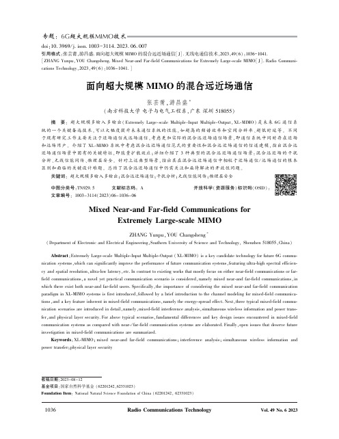
doi:10.3969/j.issn.1003-3114.2023.06.007引用格式:张芸莆,游昌盛.面向超大规模MIMO的混合远近场通信[J].无线电通信技术,2023,49(6):1036-1041. [ZHANG Yunpu,YOU Changsheng.Mixed Near-and Far-field Communications for Extremely Large-scale MIMO[J].Radio Communi-cations Technology,2023,49(6):1036-1041.]面向超大规模MIMO的混合远近场通信张芸莆,游昌盛∗(南方科技大学电子与电气工程系,广东深圳518055)摘㊀要:超大规模多输入多输出(Extremely Large-scale Multiple-Input Multiple-Output,XL-MIMO)是未来6G通信系统的一个关键备选技术,可以大幅度提升未来通信系统的性能,如超高的频谱效率和空间分辨率㊁超低时延等㊂不同于现有研究工作主要关注于近场通信或远场通信,考虑更加实际的混合远近场通信场景,即通信系统中同时存在近场和远场用户㊂介绍了XL-MIMO系统中考虑混合远近场通信范式的重要性和混合远近场通信的信道建模,指出混合远近场通信场景中固有的关键特征,即能量扩散效应;详细介绍了3种典型的混合远近场通信场景:混合远近场的干扰分析㊁无线信能同传㊁物理层安全㊂针对上述典型场景,指出其在混合远近场通信中相较于近场通信/远场通信的根本区别和面临的关键设计难题㊂总结了混合远近场通信中仍需关注和亟待解决的开放性问题㊂关键词:超大规模多输入多输出;混合远近场通信;干扰分析;无线信能同传;物理层安全中图分类号:TN929.5㊀㊀㊀文献标志码:A㊀㊀㊀开放科学(资源服务)标识码(OSID):文章编号:1003-3114(2023)06-1036-06Mixed Near-and Far-field Communications forExtremely Large-scale MIMOZHANG Yunpu,YOU Changsheng∗(Department of Electronic and Electrical Engineering,Southern University of Science and Technology,Shenzhen518055,China) Abstract:Extremely Large-scale Multiple-Input Multiple-Output(XL-MIMO)is a key candidate technology for future6G commu-nication systems,which can significantly improve the performance of future communication systems,featuring ultra-high spectral efficien-cy and spatial resolution,ultra-low latency,etc.In contrast to existing works that mostly focus on either near-field communications or far-field communications,a novel yet practical communication scenario is considered,namely mixed near-and far-field communications,in which there exist both near-and far-field users.Specifically,the importance of considering the mixed near-and far-field communication paradigm in XL-MIMO systems is first introduced,followed by a brief introduction to the channel modeling for mixed-field communica-tions,and a key feature inherent in mixed-field communications,namely the energy-spread effect.Next,three typical mixed-field commu-nication scenarios are introduced in detail,namely,mixed-field interference analysis,simultaneous wireless information and power trans-fer,and physical layer security.For above typical scenarios,fundamental differences and key design issues encountered in mixed-field communication systems as compared with near-/far-field communication systems are elaborated.Finally,open issues that deserve future investigation in mixed-field communications are summarized.Keywords:XL-MIMO;mixed near-and far-field communications;interference analysis;simultaneous wireless information and power transfer;physical layer security收稿日期:2023-08-12基金项目:国家自然科学基金(62201242,62331023)Foundation Item:National Natural Science Foundation of China(62201242,62331023)0㊀引言自2020年以来,5G移动通信系统正在全球广泛使用和部署[1-2]㊂然而,增强现实㊁全息视频和自动驾驶等新兴应用正在推动当今的5G通信系统向未来的6G移动通信系统的演进,以满足更严格的性能要求,包括前所未有的高数据速率㊁超高可靠性㊁全球覆盖㊁超密集连接等[3-6]㊂然而,现有的5G 技术可能无法完全满足这些要求,从而激发了研究6G创新技术的需求㊂而且,国际电信联盟(Interna-tional Telecommunication Union,ITU)于2023年6月发布了‘IMT面向2030及未来发展的框架和总体目标建议书“,列出了6G的定制化关键性能指标(Key Performance Indicators,KPIs),其中包含相较于5G通信系统的9个增强性能指标和6个新定义的性能指标[6]㊂值得注意的是,这些新定义的KPIs 对6G提出了更加严格的要求,因此研究6G的使能技术成为必要㊂在许多被畅想的6G使能技术中,超大规模多输入多输出(Extremely Large-scale Mul-tiple-Input Multiple-Output,XL-MIMO)已成为一项极其有前景的关键技术,可满足未来6G无线网络不断增长的性能需求,例如超高频谱效率和空间分辨率等㊂然而,6G XL-MIMO技术的使用和部署将从根本上导致电磁(Electromagnetic,EM)传播建模发生变化,即从传统的远场通信(平面波前传播)转向新的近场无线通信(球面波前传播)[7-9]㊂以XL-MIMO系统举例,其相应的电磁场可以划分为三个区域:①感应近场区域(Reactive Near-field Region);②辐射近场区域(Radiative Near-field Re-gion);③远场区域(Far-field Region)㊂现有的近场研究工作大多聚焦于辐射近场区域(也称为菲涅尔区域)㊂此外,瑞利距离(Rayleigh Distance)被广泛作为区分近场区域和远场区域的边界,其数学表达式为2D2/λ,其中D和λ分别表示天线阵列孔径和载波波长㊂值得注意的是,相较于纯近场通信或者远场通信,混合远近场通信是更为实际且极易出现的通信场景,即系统中同时存在近场用户和远场用户[10-11]㊂例如,考虑一个典型的XL-MIMO通信系统,其中配备孔径为0.5m的XL-MIMO基站以30GHz频率与用户进行通信㊂在这种情况下,众所周知的瑞利距离约为50m,约等于蜂窝系统中小区半径的一半㊂因此,考虑一些典型的通信场景,极大可能会出现一些用户位于近场区域,而其他用户位于远场区域的情况㊂而且,混合远近场通信范式的出现将会引发通信系统中新的设计难题㊂具体来说,混合远近场通信将导致一些经典通信场景的设计发生根本性的范式转变,使得针对于传统远场通信或近场通信的系统设计不再适用,因此需要根据混合远近场通信系统的特点和性能需求进行针对性设计㊂1㊀混合远近场通信基础和关键特征首先介绍混合远近场通信系统的信道模型,然后指出混合远近场通信区别于远场通信和近场通信的关键特征㊂1.1㊀远场和近场通信用户的信道模型为了清楚地展示混合远近场通信的信道模型,如图1所示,考虑一个典型的混合远近场无线通信系统,其中配备有天线数目为N的XL-MIMO基站同时服务一个单天线近场通信用户和一个单天线远场通信用户㊂下面分别给出远场用户和近场用户的信道建模过程㊂图1㊀一个典型的混合远近场无线通信系统Fig.1㊀A typical mixed-field wireless communication system 首先考虑远场用户,即到XL-MIMO基站端的距离大于定义的瑞利距离,则其信道建模遵循远场平面波传播模型,给定如下:h far=㊀N h far a(ψ),式中:h far表示远场用户和XL-MIMO基站之间的复值信道增益㊂a(ψ)表示远场信道导向矢量:a(ψ)=1㊀N[1,e jπψ, ,e jπ(N-1)ψ]T,式中:ψ=2d cos(φ)/λ表示远场用户相对XL-MIMO 基站的空间角度,φ表示信号相对于XL-MIMO基站中心的离开角(Angle of Departure,AoD),d表示天线间距㊂对于近场用户,其信道建模应遵循更为精确的球面波传播模型[12],给定如下:h near=㊀N h near b(θ,r),式中:h near表示近场用户和XL-MIMO基站之间的复值信道增益㊂b(θ,r)表示近场信道导向矢量: b(θ,r)=1㊀N e-j2π(r(0)-r)/λ, ,e-j2π(r(N-1)-r)/λ[]T,式中:θ=2d cos(ϕ)/λ表示近场用户相对于XL-MI-MO基站的空间角度,ϕ表示信号相对于XL-MIMO中心的AoD;r(n)=㊀r2+δ2n d2-2rθδn d表示XL-MIMO 基站端第n个天线到近场用户之间的距离,δn= 2n-N+12,n=0,1, ,N-1㊂值得注意的是,与远场信道导向矢量仅取决于角度不同,近场信道导向矢量同时依赖于角度和距离㊂而且,远场信道导向矢量是近场信道导向矢量的特殊形式,当用户和XL-MIMO基站间的距离大于瑞利距离时,近场信道导向矢量退化为远场信道导向矢量㊂综上所述,一个简单的混合远近场信道模型可以建模为:h mixed-field=h near+h far=㊀N h near b(θ,r)+㊀N h far a(ψ)㊂上式给出了混合场通信信道的一个简单例子,其是远场用户视距(Line-of-Sight,LoS)链路和近场用户LoS信道的叠加㊂1.2㊀混合远近场通信的固有特征:能量扩散如图2所示,混合远近场通信的一个关键特征是能量扩散效应㊂考虑在传统远场通信中被广泛采用的基于离散傅里叶变换(Discrete Fourier Trans-form,DFT)的角度域码本㊂当XL-MIMO基站选定码本中的特定码字发射定向波束以服务远场用户时,处于远场用户一定角度范围内(-0.1~0.5)的近场用户都将接收到高强度的信号㊂值得注意的是,这一独特的现象是混合远近场通信中的固有特征,其使得混合远近场通信显著区别于纯远场或近场通信㊂因此现有的针对于远场或近场通信的经典设计不再适用,使得混合场通信的专有设计成为必要㊂接下来,主要从三种典型通信场景出发,详尽地描述这些典型场景在混合场通信中相较于远场通信和近场通信的根本区别㊂图2㊀混合场通信中能量扩散效应的图解Fig.2㊀Illustration of the energy-spread effect in mixed-field communications2㊀混合远近场通信典型场景2.1㊀混合远近场通信的干扰分析考虑混合远近场通信中的多用户干扰分析[13]㊂不同于传统远场通信或近场通信中的多用户干扰产生机制,由于能量扩散效应的存在,混合远近场通信中的多用户干扰呈现出新的特点㊂具体来说,考虑不同通信场景下的多用户干扰㊂如果用户都处于传统的远场区域,空分多址接入(Spatial Division Multiple Access,SDMA)和波束分多址接入[14](Beam Division Multiple Access,BDMA)技术可以用来同时服务多个用户,并且用户间干扰较低㊂这是因为指向不同远场通信用户的定向波束在角度域上具有渐近正交性,从而有效消除用户间干扰㊂接下来,如果用户位于近场区域,新兴的位分多址接入[15](Loca-tion Division Multiple Access,LDMA)技术可以在非常低干扰下通过利用近场波束聚焦性质,同时为处于不同角度和/或距离的近场通信用户提供通信服务㊂需要强调的是,LDMA是利用近场中独特的波束聚焦效应来实现的,该效应使近场波束能够聚焦在特定的位置(范围),而不是像传统远场通信中那样波束打向特定的方向㊂然而,对于全新的混合远近场多用户通信场景,用户间的干扰分析变得非常复杂㊂为了更加清楚地描述混合场通信场景中干扰的特征,如图3所示,考虑一个典型混合场通信系统中包含一个远场用户和一个近场用户,其中XL-MIMO 基站的天线数目为256,信号传输功率为30dBm,载波频率30GHz,XL-MIMO 基站和用户的距离为7.2m㊂图3㊀近场用户的干扰功率与远场波束的空间角度的关系Fig.3㊀Interference power at a near-field user versus thespatial angle of a far-field beam一个有趣的观察是,即使近场用户位于与远场用户不同的空间角度(参见阴影区域),近场用户也会受到来自远场波束的强烈干扰,这与仅存在近场用户或远场用户场景中的结果存在显著差异㊂而且,混合远近场通信的干扰机制已经在文献[13]中进行了全面且详尽的研究㊂具体来说,远场用户对近场用户的干扰本质上是由近场用户的信道导向矢量和远场波束之间的相关性决定的,其数学描述定义为:η(θ,r ,ψ)=|b H(θ,r )a (ψ)|ʈ1N 12ðN -1n =0e jπn2d (1-θ2)2r-n θ-ψ+d (n -1)(1-θ2)2r()()㊂值得注意的是,上述定义的相关性函数可以由菲涅耳函数很好地近似,由下式给出:η(θ,r ,ψ)ʈG (β1,β2)=C ^(β1,β2)+j S ^(β1,β2)2β2,式中:β1=(θ-ψ)㊀r d (1-θ2),β2=N 2㊀d (1-θ2)r且C ^(β1,β2)=C (β1+β2)-C (β1-β2),S ^(β1,β2)=S (β1+β2)-S (β1-β2)㊂此近似的具体证明可以参考文献[13]㊂上述混合场中的干扰近似表达式给出了一个重要结果,即混合场中用户之间的干扰是由函数G (β1,β2)以及两个参数β1和β2给出的㊂更具体地说,β1是远场用户的空间角度㊁近场用户的空间角度和距离的函数,而β2则由XL-MIMO 基站的天线数目以及近场用户的角度和距离共同决定㊂文献[13]针对这些关键参数对混合场干扰的具体影响已经进行了全面而详尽的研究㊂总的来说,当XL-MIMO 基站的天线数量和近场用户距离相对较小,和/或近场用户和远场用户空间角度差较小时,用户间存在强干扰[13]㊂综上所述,混合远近场通信中独特且固有的能量扩散效应将不可避免地导致更为复杂的多用户干扰问题,也为后续的干扰消除方案设计带来严峻的挑战㊂2.2㊀混合远近场通信的无线信能同传从无线使能通信(Wireless Power Transfer,WPT)的角度来看,混合远近场通信的能量扩散效应可以被利用来提升系统能量采集性能[16]㊂具体来说,为远场通信用户服务的基于DFT 的波束引起的能量泄漏可以被利用为近场能量采集用户充电㊂特别地,考虑一个典型的混合场无线信能同传场景(Simultaneous Wireless Information and Power Trans-fer,SWIPT),其中能量采集(Energy Harvesting,EH)用户和信息解码(Information Decoding,ID)用户分别假设位于XL-MIMO 系统的近场和远场区域㊂需要强调的是,混合远近场SWIPT 的系统设计也面临着新的挑战㊂例如,通过利用近场波束聚焦特性,近场EH 用户的波束赋形应精心设计,以最大限度地提高EH 效率,同时最大可能地减少对远场ID 用户的干扰㊂在为远场ID 用户设计波束赋形时应充分利用能量扩散效应,当近场EH 用户与远场ID 用户位于相似的角度时,服务于远场用户的波束可以机会性地为近场EH 用户充电㊂此外,应精心设计基站的功率分配,以平衡混合场SWIPT 系统中新的远近权衡与波束聚焦和能量扩散的影响㊂现有的研究工作[16]表明,混合场SWIPT 系统中的波束调度显著不同于传统远场SWIPT系统的波束调度设计㊂具体而言,如图4所示,混合场SWIPT 系统的最优设计需要调度近场EH 用户,而远场SWIPT 系统最优设计表明只需调度ID 用户[17]㊂图4㊀混合场SWIPT系统波束调度图Fig.4㊀Illustration of beam scheduling in mixed-field SWIPT 2.3㊀混合远近场通信的物理层安全考虑混合场物理层安全(Physical Layer Security, PLS)㊂针对于传统的远场PLS,在角度域区分合理用户和窃听用户即可实现安全通信[18]㊂对于新兴的近场PLS,通过利用近场通信所带来的额外的距离域分辨率,处于同一空间角度而不同距离的合理用户和窃听用户也可实现安全通信[19]㊂然而,针对于混合场PLS,实现安全通信极具挑战性㊂具体来说,考虑一类具有挑战性的混合场PLS通信场景,即窃听用户位于XL-MIMO系统的近场区域,而合理用户处于远场区域㊂在这类场景中,由于窃听用户可以在一定范围内从合理用户的信息泄漏(Information Leakage)中窃听合理用户的信息,同时处于近场的窃听用户享有更好的信道条件,因此针对这类场景的混合场PLS极具挑战性,这也凸显了混合场PLS方案设计的必要性㊂3㊀混合远近场通信开放性研究问题3.1㊀混合远近场通信的信道建模信道建模为混合远近场通信奠定了基础㊂在现有的研究工作中,广泛假设混合场信道模型由近场和远场LoS信道组成㊂然而,需要研究更实际和通用的混合远近场信道模型㊂例如,研究用于混合远近场通信的更复杂的多径信道至关重要,该信道建模考虑了XL-MIMO系统远场和/或近场中周围环境散射体引起的多径㊂同时,混合远近场通信中可视区域[20](Visible Region,VR)现象也会更加显著㊂这是因为除了环境散射体会影响不同用户的VR,近场和远场之间的相互作用也会进一步使不同用户的VR复杂化,需要正确建模这种影响㊂此外,除了确定性信道模型之外,近场信道模型多呈现出近场空间相关性和非平稳性㊂因此,混合远近场的信道建模也需要考虑随机性的近场信道模型㊂3.2㊀混合远近场通信的波束管理为了实现高质量的通信服务,混合远近场通信的波束管理也至关重要[10]㊂具体来说,现有的波束训练方法假设用户全部位于远场区域或近场区域㊂对于混合远近场通信场景下用户同时分布在近场和远场区域,如何设计适用于近场和远场通信场景的统一波束训练方法是一个关键问题㊂这需要进一步深入研究近场和远场波束训练方法的有效融合㊂而且,对于混合远近场的波束追踪,考虑远场和近场用户的高移动性,远场用户可能会进入近场区域,近场用户也可能进入远场区域㊂这在设计混合场波束追踪算法时需要同时考虑对用户所处场的预测,以及相应的波束追踪算法设计㊂混合场的波束调度也是一个实际而具有挑战性的问题㊂由于混合场通信场景中存在新的远近均衡(Near-to-Far Tradeoff),因此在设计混合场波束调度方法时需要精巧地设计以达到一个系统的均衡㊂3.3㊀混合远近场通信的收发器设计由于XL-MIMO系统通常工作在高频段,高功耗和硬件复杂性成为核心问题㊂一个理想的解决方案是利用经典的混合波束成形技术来降低硬件和能源成本[21]㊂然而,随着XL-MIMO天线数目的增加,经典的混合波束成形技术仍然具有很高的复杂度㊂因此,考虑采用子连接架构㊁动态子阵列架构和透镜天线阵列等进行适当设计,以实现复杂度和性能之间的权衡㊂由于混合场通信系统中同时存在近场和远场用户,因此需要考虑新型的收发器结构设计,使之可以同时服务于两类用户㊂此外,高频率伴随的高宽带会在近场通信中产生波束分裂现象(Beam Split),现有的基于移相器的模拟组件无法处理此问题㊂一种有效的解决方案是在射频链路和移相器之间采用额外的电路来生成与频率相关的相移,从而将波束聚焦在整个带宽上㊂这个方向仍处于早期阶段,值得进一步研究在射频链和移相器之间采用额外的真时延[22](True Time Delay,TDD)电路来产生与频率相关的相移,从而将波束聚焦在整个带宽上㊂4 结论主要考虑6G XL-MIMO系统中一个典型且实际的混合远近场通信场景,即系统中同时存在近场用户和远场用户㊂针对这一新兴通信范式,强调了6G XL-MIMO系统中考虑此范式的重要性㊂介绍了其固有的能量扩散现象㊂考虑了混合场通信的三种典型场景:混合场干扰分析㊁SWIPT和PLS,并着重阐述混合远近场通信中三种典型场景和传统远场及近场通信的基本区别和新的设计思路㊂总结了混合远近场通信需要研究和亟待解决的几个关键问题㊂参考文献[1]㊀ANDREWS J G,BUZZI S,CHOI W,et al.What will5Gbe?[J].IEEE Journal on Selected Areas in Communica-tions,2014,32(6):1065-1082.[2]㊀SHAFI M,MOLISCH A F,SMITH P J,et al.5G:A TutorialOverview of Standards,Trials,Challenges,Deployment,and Practice[J].IEEE Journal on Selected Areas in Com-munications,2017,35(6):1201-1221.[3]㊀张平,牛凯,田辉,等.6G移动通信技术展望[J].通信学报,2019,40(1):141-148.[4]㊀邵泽才,袁弋非,李娜,等.6G网络能耗面临的机遇与挑战[J].无线电通信技术,2023,49(3):385-392. [5]㊀王承祥,黄杰,王海明,等.面向6G的无线通信信道特性分析与建模[J].物联网学报,2020,4(1):19-32. [6]㊀YOU X H,WANG C X,HUANG J,et al.Towards6GWireless Communication Networks:Vision,EnablingTechnologies,and New Paradigm Shifts[J].中国科学:信息科学(英文版),2021,64(1):5-78.[7]㊀TU-R WP5D.Recommendation ITU-R M.[IMT.Frame-work for2030and Beyond].[EB/OL].[2023-08-10].https:ʊwww.itu.int/md/R19-WP5D-C/en. [8]㊀WANG Z,ZHANG J,DU H,et al.Extremely Large-scaleMIMO:Fundamentals,Challenges,Solutions,and FutureDirections[J/OL].(2023-04-06)[2023-07-26].https:ʊ/abs/2209.12131.[9]㊀CUI M,WU Z,LU Y,et al.Near-field MIMO Communica-tions for6G:Fundamentals,Challenges,Potentials,andFuture Directions[J].IEEE Communications Magazine,2022,61(1):40-46.[10]YOU C,ZHANG Y,WU C,et al.Near-field Beam Man-agement for Extremely Large-scale Array Communications[J/OL].(2022-01-22)[2023-08-10].https:ʊarxiv.org/abs/2306.16206.[11]HAN C,CHEN Y,YAN L,et al.Cross Far-and Near-fieldWireless Communications in Terahertz Ultra-large AntennaArray Systems[J/OL].(2023-08-03)[2023-08-10].https:ʊ/abs/2301.03035.[12]ZHANG Y,WU X,YOU C.Fast Near-field Beam Trainingfor Extremely Large-scale Array[J].IEEE Wireless Com-munications Letters,2022,11(12):2625-2629. [13]ZHANG Y,YOU C,CHEN L,et al.Mixed Near-and Far-field Communications for Extremely Large-scale Array:An Interference Perspective[J/OL].(2023-01-29)[2023-08-10].https:ʊ/abs/2301.07277.[14]SUN C,GAO X,JIN S,et al.Beam Division MultipleAccess Transmission for Massive MIMO Communications[J].IEEE Transactions on Communications,2015,63(6):2170-2184.[15]WU Z,DAI L.Multiple Access for Near-field Communica-tions:SDMA or LDMA?[J].IEEE Journal on SelectedAreas in Communications,2023,41(6):1918-1935. [16]ZHANG Y,YOU C,YUAN W,et al.Joint Beam Schedu-ling and Power Allocation for SWIPT in Mixed Near-andFar-field Channels[J/OL].(2023-04-17)[2023-08-10].https:ʊ/abs/2304.07945. [17]XU J,LIU L,ZHANG R.Multiuser MISO Beamforming forSimultaneous Wireless Information and Power Transfer[J].IEEE Transactions on Signal Processing,2014,62(18):4798-4810.[18]吴宣利,许智聪,王禹辰,等.基于信道相关性的物理层安全性能分析[J].通信学报,2021,42(3):65-74. [19]DONG Z,ZENG Y.Near-field Spatial Correlation forExtremely Large-scale Array Communications[J].IEEECommunications Letters,2022,26(7):1534-1538. [20]HAN Y,JIN S,WEN C K,et al.Channel Estimation forExtremely Large-scale Massive MIMO Systems[J].IEEEWireless Communications Letters,2020,9(5):633-637.[21]YU X,SHEN J C,ZHANG J,et al.Alternating Minimiza-tion Algorithms for Hybrid Precoding in Millimeter WaveMIMO Systems[J].IEEE Journal of Selected Topics inSignal Processing,2016,10(3):485-500. [22]崔铭尧,谭竞搏,戴凌龙.面向信道簇模型的太赫兹宽带混合预编码[J].中国科学(信息科学),2023,53(4):772-786.作者简介:张芸莆㊀男,(1995 ),南方科技大学访问研究生㊂主要研究方向:智能反射面㊁近场通信㊂(∗通信作者)游昌盛㊀男,(1991 ),博士,助理教授㊂主要研究方向:智能反射面㊁近场通信㊂。
西电宽带无线通信课件第一章 绪论(概述) (12年)

HSPA+
HSDPA (P1)
1.8M/3.6Mbps
HSDPA(P2)
7.2/14.4Mb/s
DL:>40Mbps UL>10Mbps
LTE
DL:100Mbps UL:50Mbps
384kb/s
HSUPA
6-8Mbps
TD-SCDMA无线技术演进路线
GSM/GPRS/EDGE
171kb/s/384kbps
国家重点实验室
Broadband Wireless Communications
(宽带无线通信)
盛敏 杨春刚 msheng@
国家重点实验室
课程的基本信息
• 课程编号: 0142228(专业) • 课程名称:宽带无线通信 • 硕士生选修课 • 课内学时数:46学时 • 上课时间:( 地点:J2-04) • 授课方式:讲课、自学、研讨 • 考试方式:笔试 • 先修课程:移动通信或个人无线通信
1995 2000 2005 HSDPA HSUPA 1xEV-DO 2010 2015 LTE DO Rev C
移动性
1985
商用时间
GSM cdmaOne
高 1G 中
AMPS TACS
E3G 3G
3G增强型
(3G演进型)
IMT-Advanced 4G
2G
WCDMA R99/R4 cdma2000 1X TD-SCDMA R4
国家重点实验室
教学目标
要求学生掌握宽带无线通信系统的基本原理、
主要的理论和技术,为设计和研究新型无线通信系 统打下良好的基础。通过本课程的学习,应当能就 本课程相关的专题写出有创新的研究报告。
国家重点实验室
An Approximate Capacity Distribution for MIMO Systems

IEEE TRANSACTIONS ON COMMUNICATIONS, VOL. 52, NO. 6, JUNE 2004887An Approximate Capacity Distribution for MIMO SystemsPeter Smith and Mansoor ShafiAbstract—In this letter, we derive the exact variance of the capacity of a multiple-input multiple-output (MIMO) system. This enables an investigation of the accuracy of a Gaussian approximation to the capacity foreshadowed by various central limit theorems. We confirm recent results which state that the capacity variance appears to converge to a limit independent of absolute antenna numbers, but dependent on the ratio of the numbers of receive to transmit antennas. The Gaussian approximation itself is surprisingly good, even in the worst cases giving satisfactory results. Index Terms—Capacity, central limit theorem, multiple-input multiple-output (MIMO), Rayleigh channel.A closed-form formula for the variance is developed in the Appendix, in the form of a single numerical integral. In summary, the Gaussian approximation to channel capacity is a simple and powerful tool to enable engineering estimates of system capacity, total throughput, and capacity outage probability. The rest of the letter is laid out as follows. In Section II, we give some background and review the relevant literature. In Section III, we discuss central limit theorems (CLTs) for the capacity and provide the methodology for the Gaussian approximation. In Section IV, results are given and in Section V, conclusions are presented. II. BACKGROUND A. Link and Channel Model Consider a transmission system where each user transmits simultaneously via antennas, and reception is via antennas. We , . The define , to be given by total power of the complex transmitted signal is constrained to , regardless of the value of . The received signal in this complex -dimensional system is (1) where is a complex channel-gain matrix. For uncorrelated Rayleigh fading, the entries in are independent and identically distributed (i.i.d.), complex, zero-mean Gaussians with unit magnitude variance. In (1), is a complex -dimensional additive white Gaussian noise (AWGN) vector, with statistically independent components of identical power at each without loss of of the receive branches. We assume generality. Assuming a narrowband channel, the matrix channel response may be assumed constant over the band of interest, a frequency-flat channel. The relevant capacity for such a channel is expressed as [1]–[3] b/s/Hz (2)I. INTRODUCTIONMULTIPLE-INPUT multiple-output (MIMO) systems have recently been a subject of intense research activity [1]–[3]. Our work focuses on MIMO capacity, and we take the well-known quasi-stationary channel approach [1], which leads to the concept of capacity as a random variable. From a system engineer’s viewpoint, we would therefore like to know: 1) what the mean system capacity is, and how this varies with the number of transmit and receive antennas and receiver signal-to-noise-ratio (SNR); 2) what the variance of the capacity is and how this varies with the numbers of transmit/receive antennas and SNR; 3) what the probability density function (pdf) of the system capacity is so that percentages of time capacity below a certain threshold (known as capacity outage) may be estimated. Telatar [3] has derived an exact expression for the mean system capacity of a MIMO system, and Rapajic and Popescu [4] have evaluated the limiting mean system capacity for large arrays. Results on the variance and the pdf of channel capacity are only recently emerging. Hence, in this letter, we show that: 1) the channel capacity of a MIMO system can be accurately modeled by a Gaussian random variable. The exact mean and variance of the capacity are given for any numbers of transmit and receive antennas; 2) the variance of the channel capacity is not sensitive to the number of antennas and is mainly influenced by the SNR.idenwhere denotes transpose conjugate, denotes an tity matrix, and we assume equal power transmission on the transmit antennas. B. Moments In [3], Telatar has derived an exact expression for the mean of the system capacity given byPaper approved by N. C. Beaulieu, the Editor for Wireless Communication Theory of the IEEE Communications Society. Manuscript received May 2, 2001; revised January 6, 2003 and November 19, 2003. This paper was presented in part at the IEEE International Conference on Communications, New York, NY, April 28–May 2, 2002. P. Smith is with the Department of Electrical and Computer Engineering, University of Canterbury, Christchurch, New Zealand (e-mail: p.smith@). M. Shafi is with Telecom New Zealand Limited, Wellington, New Zealand (e-mail: mansoor.shafi@). Digital Object Identifier 10.1109/TCOMM.2004.829557(3)0090-6778/04$20.00 © 2004 IEEE888IEEE TRANSACTIONS ON COMMUNICATIONS, VOL. 52, NO. 6, JUNE 2004where are generalized Laguerre polynomials of order . In the limit as , , and is held constant, the mean capacity has been shown to converge to [4] (4) where , , , andNote that Rapajic and Popescu [4] also show how to interchange and so that (4) can always be used, whether or . In terms of higher order moments, results are now appearing [5], [6] which give various limiting results for the variance. They show that the capacity variance converges to a constant as , , and is held constant. This limiting variance depends only on the ratio of and , and not on their individual values. However, to the best of our knowledge, no exact results are available for the variance. Hence, we derive the variance in Section III below.Fig. 1. Mean capacity versus antenna number for r= t.III. METHODOLOGY We use relatively little-known CLTs for random matrices [7] which may be applied in the complex case to the capacity variable. Now it is known from [7, pp. 278–310] that a certain CLT exists which states that the distribution of the standardized ca, and pacity is asymptotically Gaussian as for some constant . The standardized capacity is simply the capacity shifted and scaled to have zero mean and unit variance. In other words, if is the capacity variable with mean and standard deviation , then the standardized capacity . To implement the Gaussian approximation, we reis and . The exact mean was given in [3], see quire (3), and the limiting value in [4], see (4). The variance is derived here in the Appendix following Telatar’s approach, and is given in two formsFig. 2. Variance of capacity versus antenna number for r= t.where polynomial, and,is a generalized Laguerre(7)(8) (5) Hence, the variance can be found by double numerical integration using (5), or several single numerical integrations via (6). In this letter, we have used (6) in all the results. IV. RESULTS Fig. 1 shows the useful result that over the whole range of , , and SNR considered the Rapajic limiting mean value [4] is visually indistinguishable from Telatar’s exact mean [3] (at least on this scale of plot). Also demonstrated is the well-known linear with . Fig. 2 shows the behavior of the cagrowth of pacity variance for and various SNR values. It shows that increases for any SNR value, the variance stabilizes as(6)IEEE TRANSACTIONS ON COMMUNICATIONS, VOL. 52, NO. 6, JUNE 2004889. The Gaussian approxinumbers, but dependent on the ratio mation itself is surprisingly good, even in the worst cases giving satisfactory results. APPENDIX DERIVATION OF THE VARIANCE OF THE CAPACITY We follow the derivation of the mean capacity given by Telatar [3] and extend this approach to the variance. Let denote the eigenvalues of for and for . Then from (1), we haveFig. 3. Comparison of simulated capacity with a normal approximation (SNR 3 dB).=The variance ofis given by(9) is a pair where is a randomly selected eigenvalue, and of randomly selected (distinct) eigenvalues. Using the notation , we haveFig. 4.= 15 dB).Comparison of simulated capacity with a normal approximation (SNR(10) , The main difficulty in (10) is the evaluation of for which we need the joint density of , . Telatar [3] gives as the joint density ofalthough this stabilization occurs more rapidly for small SNR. These experimental results support the limiting variance results in [5] and [6]. Gaussian approximations to the capacity distribution can now be investigated, since we have results for the mean and variance. Note that the mean is straightforward to compute either by Rapajic’s closed-form limiting value (4) or by a single well-behaved numerical integration (3). Figs. 3 and 4 show the accuracy of a Gaussian approximation to the reliability function or complementary cumulative distribution func. The Gaussian approximation does remarktion ably well over the whole range of and values, considering the CLT only offers Gaussianity as , . When , the Gaussian approximation is virtually indistinguishable from the simulated curve, and accurately predicts the capacity percentiles. The worst fits occur for high SNR and low values of . However, even the worst fit, in Fig. 4, is fairly respectable. V. CONCLUSIONS We have derived the variance of the capacity of a MIMO system, allowing an investigation of the accuracy of a Gaussian approximation to capacity foreshadowed by various CLTs. We confirm recent results which state that the capacity variance appears to converge to a limit independent of absolute antenna(11) where the sum is over all possible permutations of , denotes the sign of the permutation, and is given by (12) is a generalized Laguerre polynomial. Since are unordered, we can obtain the joint density of , by integrating (11) over and using the orthogonality relationship [3] whereThis approach gives the joint density of,as(13)890IEEE TRANSACTIONS ON COMMUNICATIONS, VOL. 52, NO. 6, JUNE 2004Identifying the nonzero terms in (13) (where substituting (12) gives) and(17) The integrals in (17) appear to be intractable in closed form. The first single integral can be rewritten in terms of special functions, but the formulation as an integral is just as convenient, since the integrand is well behaved and numerical integration is straightforward. The double integral can also be evaluated numerically, outside the inteor we can take the summations in grals to give(14) With a little rearrangement, (14) can be rewritten as (15) where is the density of an arbitrary eigenvalue given by Telatar [3] asand (18) Hence, we can either perform the single double-numerical integration in (17) or several single-numerical integrations in (18). Results in this letter were calculated using (18). Now we can turn to the calculation of since REFERENCES[1] G. J. Foschini and M. J. Gans, “On limits of wireless communication in a fading environment when using multiple antennas,” Wireless Pers. Commun., vol. 6, pp. 311–335, Mar. 1998. [2] G. J. Foschini, “Layered space–time architecture for wireless communication in a fading environment when using multielement antennas,” Bell Labs Tech. J., vol. 1, no. 2, pp. 41–59, 1996. [3] I. E. Telatar, “Capacity of multiantenna Gaussian channels,” Eur. Trans. Telecommun., vol. 10, no. 6, pp. 586–595, Nov./Dec. 1999. [4] P. B. Rapajic and D. Popesu, “Information capacity of a random signature multiple-input multiple-output channel,” IEEE Trans. Commun., vol. 48, pp. 1245–1248, Aug. 2000. [5] A. M. Sengupta and P. P. Mitra, “Capacity of multivariate channels with multiplicative noise: I. Random matrix techniques and large-n expansions for full transfer matrices,” LANL arXiv:physics/0010081, Oct. 31, 2000. [6] E. Biglieri and G. Tarico, “Large-system analysis of multiple-antenna system capacities,” J. Commun. Networks, vol. 5, no. 2, pp. 96–103, June 2003. [7] V. L. Girko, Random Matrices. Kiev, Ukraine: Kiev Univ. Press, 1975.(16) Substituting (16) in (10) gives。
毕业设计英文翻译——认知无线电频谱感知算法仿真要点

*仅供参考上海电力学院毕业设计(英文翻译)课题名称认知无线电频谱感知算法仿真院(系)专业班级学生学号Implementation Issues in Spectrum Sensing for Cognitive Radios认知无线电频谱感知的实现问题Abstract:There are new system implementation challenges involved in the design of cognitive radios, which have both the ability to sense the spectral environment and the flexibility to adapt transmission parameters to maximize system capacity while co-existing with legacy wireless networks. The critical design problem is the need to process multi-gigahertz wide bandwidth and reliably detect presence of primary users. This places severe requirements on sensitivity, linearity, and dynamic range of the circuitry in the RF front-end. To improve radio sensitivity of the sensing function through processing gain we investigated three digital signal processing techniques: matched filtering, energy detection, and cyclostationary feature detection. Our analysis shows that cyclostationary feature detection has advantages due to its ability to differentiate modulated signals, interference and noise in low signal to noise ratios. In addition, to further improve the sensing reliability, the advantage of a MAC protocol that exploits cooperation among many cognitive users is investigated.摘要:出现了一些新系统的实施挑战,其涉及认知无线电——具有感知频谱环境下的传输参数既适应能力和灵活性,以最大限度地提高系统容量,同时并存于传统无线网络。
室内大尺度参数特性测量

Large Scale Parameters and Double-Directional Characterization of Indoor Wideband Radio Multipath Channels at11GHz Minseok Kim,Member,IEEE,Yohei Konishi,Student Member,IEEE,Yuyuan Chang,andJun-ichi Takada,Senior Member,IEEEAbstract—This paper presents the large scale parameters of wideband multipath channels based on extensive measurement campaigns in various indoor environments.The measurements were conducted with a wideband multiple-input multiple-output (MIMO)channel sounder having a bandwidth of400MHz at11 GHz which is a challenging frequency for future mobile systems. In particular,polarization characteristics of path-loss,shadowing, cross-polarization power ratio(XPR),delay spread and coher-ence bandwidth are characterized.The measurement results show that the path-loss exponents range between2.0and3.0 for none-line-of-sight(NLoS),0.36and1.5for LoS,respectively. Vertically and horizontally polarized transmissions have almost same path-gain,but in some corridor-room NLoS environments, the path-loss for HH is significantly large.In most cases,the RMS delay spreads are less than20and50ns for NLoS and LoS,respectively,and the average coherence bandwidth is less than30MHz.The Rician-factors range between2and3dB for cross-polarization,and in large Hall environments,those for co-polarization are greater than6.0dB with10%probability. Finally,some dominant propagation mechanism and site-specific behaviors are illustrated using the double-directional measure-ment results.Index Terms—Delay spread,indoor,path-loss,radio propaga-tion,shadowing,wideband,11GHz.I.I NTRODUCTIONA S the data traffic in mobile Internet services has been dra-matically increasing because of the explosion in usage of smartphones and tablet devices,conventional cellular networks covering large cell area cannot be expected to provide sufficient capacity and satisfactory data rates.In recent3G cellular sys-tems universally available portable services have been realized, and data rates of approximately several tens of megabits per second can be experienced in the current LTE/LTE-A systems. However,tremendous data traffic will still be a major concern for future mobile systems.Because of the technical challenges in increasing the capacity and data rates to a much greater de-gree,there has been an increasing interest in deploying relays,Manuscript received July30,2013;revised September24,2013;accepted October25,2013.Date of publication November05,2013;date of current ver-sion December31,2013.This work was supported in part by the Research and Development Project for Expansion of Radio Spectrum Resources of The Min-istry of Internal Affairs and Communications,Japan.The authors are with the Graduate School of Science and Engineering,Tokyo Institute of Technology,Tokyo,Japan(e-mail:mskim@).Color versions of one or more of thefigures in this paper are available online at .Digital Object Identifier10.1109/TAP.2013.2288633distributed antenna systems,and small cell communications in densely populated areas[1],[2].In addition,further increase in frequency bandwidth will be necessary.However,because of the serious congestion of the frequency spectrum at lower microwave bands(below5GHz), exploring new frequency bands above5GHz is an inevitable choice in the future.These higher frequency bands were previ-ously neglected by land mobile researchers because of their high path-loss with distance[3],[5].Further,deep shadowing due to weak diffraction and higher Doppler frequency are expected. Thus,using high frequency bands has been considered disad-vantageous in mobile transmission.However,the radio propa-gation properties at higher frequency bands have not been suf-ficiently justified from the view point of the requirements for current mobile data transmission.In fact,a large path-loss is not always a disadvantage,and can be an advantage when de-signing small cell or hot spot systems within a confined cov-erage area where very high-speed data transmission can be re-alized because a very wide frequency bandwidth is available. Thus,extensive measurement based characterization of the radio propagation properties at higher frequency bands is neces-sary to determine the operation strategy and to design the system parameters.In small cell environments,the channel behaviors should be quite site-specific depending on the individual en-vironments,so that the design and analysis of the system re-quire more sophisticated channel models of correlation among the multiple links in relay,distributed antennas,and other coop-erative schemes,and a possible rank of the multiple-input mul-tiple-output(MIMO)channels.This work presents the radio channel characteristics over wide bandwidth of400MHz with the carrier frequency of11 GHz which has been chosen assuming a mobile system with an area smaller than the conventional microcell coverage area[1], [2].Although a large number of studies have been conducted on the radio channel for mobile systems below5GHz,to our best knowledge,only few measurements and analyses at around11GHz have been found[4]–[8].In1989,some basic propagation experiments were conducted on the path-loss characteristics in microcell environments having a low base station antenna height at11GHz[4].In[5],a measurement at 10GHz was conducted and a statistical model of small-scale fading in some indoor environments was presented.In[6],[7], Janssen et al.conducted extensive measurements in an indoor office environment at2.4,4.75,and11.5GHz,and provided some insights on channel characteristics such as path-loss,0018-926X©2013IEEEroot-mean-square(RMS)delay spread,and coherence band-width from the comparative analyses of the three frequencies.A large path-loss in obstructed line-of-sight(OBS)situations and small delay spread(515ns)observed at11.5GHz over the other two frequencies.Additionally,a comparative study on the coherence bandwidth at11.2and62.4GHz for indoor line-of-sight(LoS)microcells has been presented in[8]. Because the polarization characteristics of the radio channel are important for polarization diversity with co-located an-tennas,the polarization effects in an indoor environment at various frequency bands have been discussed,[9]–[17].Orthog-onally polarized MIMO systems use low correlation between two polarizations,so the orthogonally polarized antennas can be co-located to enable the design of a compact antenna system. Because the two orthogonal polarization components of an electromagnetic wave are independent,the correlation between antennas for different polarizations will also be low with low coupling with each other.Comparing with existing studies mentioned above,the orig-inal contribution of this paper is to present the polarization behaviors of the large scale parameters at a new challenging frequency band of11GHz.Specifically,this paper presents them based on extensive measurement campaigns in various in-door environments of the university building in Tokyo Institute of Technology,Japan.The measurements have been conducted with a wideband MIMO channel sounder having a bandwidth of400MHz at11GHz[19].The instantaneous channel transfer functions were taken using dual-polarized dipole antennas on both sides of the transmitter and the receiver.This paper presents the most fundamental parameters,which describe the dominant characteristics of the environment,including path-loss,shadowing,and RMS delay spread,and coherence bandwidth in terms of the polarization.In addition,the mea-sured narrowband Rician-factors will also be discussed to describe the contribution of thefixed coherent component in the measurement environments.Finally,the dominant propa-gation mechanism and site-specific behavior of the individual environment will be illustrated using the double-directional measurement results.The remainder of this paper is organized as follows.The measurement campaign including the MIMO channel sounder and measurement environments are described in Section II. Section III presents the large scale parameters;path-loss, shadowing,cross polarization power ratio(XPR)/co-polariza-tion power ratio(CPR),RMS delay spread,and coherence bandwidth.Next,the narrowband Rician-factors of each environment are presented in Section IV.Then,the dominant propagation mechanism with double-directional measurement results are discussed in Section V.Finally,conclusions and a summary of the results are given in Section VI.II.M EASUREMENT C AMPAIGNA.MIMO Channel SounderFor the measurements,dual-polarized,namely,vertically polarized(VP)and horizontally polarized(HP),dipole an-tennas having an omni-directional azimuth radiation pattern with a gain of4dBi were used.The half beam width inTABLE IC HANNEL S OUNDING PARAMETERSthe vertical pattern was35degrees.The triple-link124 dual-polarized MIMO channel measurement was configured with a12-element(6VP/HP)linear array at the transmitter and4-element(2VP/HP)antenna array at the three receivers, respectively.Table I shows the measurement parameters in detail.The antenna spacing of the array was approximately, and the transmitting power per antenna was10dBm.In the channel sounder,the channel transfer functions(TFs)of2,048 sub-carriers over400MHz bandwidth were measured in a single snapshot by transmitting an unmodulated multitone signal[19].The noisefloor in the path gain measurement was approximately91dB with respect to the level(0dB)in the back-to-back direct connection between the transmitter and the receiver.By inverse discrete Fourier transform(IDFT)of the TFs,the impulse response(IR)of the-th snapshot for the-th transmit antenna to the-th receive antenna is obtained as(1) where and denote discrete frequency and delay indices, respectively.Here,is a window function that reduces the side lobe effect in estimating the IR and the correction factor.denotes the transfer function of the -th the-th transmit antenna to the-th receive an-tenna.It should be noted that the sum power of IR in the delay domain is equal to the mean power of TF in the frequency do-main from Parseval’s theorem as(2) The noise level in IR is approximately124dB with a matched filter gain of33dB.The maximum measurable excess delay is4.Fig.1.MIMO channel sounder configurations.(a)MIMO channel measure-ment.(b)Double-directional channel measurement.The MIMO channel sounder has a fully parallel transceiver architecture that employs a layered scheme of frequency divi-sion multiplexing(FDM)and space-time division multiplexing (STDM).Fig.1shows the photographs of the channel sounder where the number of antennas is scalable by a combination of multiple transceiver units,and there isflexibility for both the multi-link(ML)MIMO channel measurement shown in Fig.1(a)and the double-directional channel measurement shown in Fig.1(b)[19],[20].The frequency and time synchro-nizations between the units were precisely taken with a cesium atomic clock(accuracy:).In fact,the measurement of all the MIMO sub-channels of the three links were taken si-multaneously.However,in this paper,multiple MIMO channel responses were used to characterize the large-scale parameters through spatial averaging.B.Measurement EnvironmentsIn the following scenarios,the specified number of snapshots were obtained by moving the transmitter slowly along the routes at a constant speed(0.25m/s).At the speed the Doppler phase shift is negligibly small.The surrounding environment was maintained to be static during a measurement.In each environment,the ML channel measurement was conducted by synchronizing two or three different receiver units and simultaneously measuring all the MIMO sub-channels of those links.The dimensions and conditions of the environments in NLoS and LoS scenarios are presented in Table II.1)NLoS Scenarios(Corridor-Room):For NLoS scenarios, the measurement campaign was carried out at thefirst level of the lecture building.It mainly consists of a30-m-long corridor, some lecture rooms,a meeting room,and some laboratories.The walls between the rooms were constructed with plasterboards, but those between the corridor and the rooms were constructed with reinforced concrete.Thefloor was made of reinforced con-crete.Thefloor plan is depicted in Fig.2(a).220snapshots wereTABLE IIM EASUREMENT E NVIRONMENTSobtained at every14cm(about)by moving the transmitter along the corridor(Route1).Two receivers with a dual-polar-ized4-element antenna array(2V/H)were located at two dif-ferent points of RxA and RxB in Room A and Room B,respec-tively.Further,the area of Room B was twice that of Room A, and the metallic doors of Room A and B were opened,but those of others were closed.As can be expected from thefloor plan in Fig.2(a),all the measurement points are in NLoS for Room A,but they can be divided into the following three parts for Room B as:•NLoS(Area1):the transmitter was located in the corridor and there was no LoS path.•LoS:the receiver could see the transmitter through the open door.•NLoS(Area2):there were a rest room and an entrance area in the vicinity of the transmitter.Because of the differences in the surrounding environments,the NLoS channels for Area1and2were separately characterized.2)LoS Scenarios:The measurement was also conducted in three different LoS environments,as shown in Fig.2(b)and(c), where Room C,Hall D and Hall E denote a medium scale lecture room having a metal platefloor,an entrance hall,and a large event hall,respectively.In Room C,two metallic white boards are installed on the front and rear side walls,and a part of the wall is also made of metal,as shown in Fig.2(b).Similar to the NLoS measurements,220,440,and390snap-shots were taken by moving the transmitter along the routes in the scenarios of Room C(Route2and3),Hall D(Route4and 5)and Hall E(Route6and7),respectively.During the mea-surement of Hall D and Hall E,in some instances,there were people passing by or resting in chairs.III.C HARACTERIZATION OF L ARGE S CALE P ARAMETERSA.Path-Loss and ShadowingThe polarimetric path gain was calculated by averaging the local path gains(PGs)of all the MIMO channels over the entire bandwidth as(3) where and can take either horizontal(‘H’)or vertical(‘V’) polarizations,and and denote the sets of the transmit and the receive antenna indices for the and polarizations,respec-tively.Further,denotes the maximum delay index of the power level greater than the noise level.For all the cases,256 delay samples from the zero delay were used,Fig.2.Floor plan views of the measurement environments (Tx moved slowly along the routes at constant speed)where ‘’s on the routes denote the Tx positions for further analysis in the subsequent sections.(a)NLoS (Room A and Room B);(b)LoS (Room C and Hall D);(c)LoS (HallE).Fig.3.Measured PL and PL models of indoor NLoS measurement (Corridor-Room).(a)Co-polarization.(b)Cross-polarization.which is equivalent to 640ns in the continuous delay domain.In addition to averaging over spatial and frequency domains in (3),averaging a few snapshots further eliminated a small scale fading effect,and then,the path-loss for each polarization pair was calculated from the reciprocal of the path gain.It should be noted that the total antenna gain of 8dBi at both the transmit and receive sides was excluded from the path-loss.The measured path-losses of the NLoS and LoS conditions for each polarization pair are shown in Figs.3and 4,respec-tively,where the path gains were averaged within approximately 0.5m .For each case,the path-loss was characterized using the measurement data.The measured path-losses were lin-early fitted into the widely accepted power-law model by plot-ting the path-loss (PL)in terms of the distance between the transmitter and the receiver on the log-log scale as(4)where and denote the path-loss exponent and the intercept at 1m distance,respectively.Here,indicates a log-normally distributed random variable with zero mean and variance .The fitted models are plotted in Figs.3and 4where the free space path-lossis shown with a dashed line for reference,and the model parameters are summarized in Table III.The propagation mechanism for the NLoS channel between the corridor and Room A involves the propagation of the trans-mitted waves along the corridor with a number of sidewall re-flections that then flow into the room.The waves are also accu-mulated after re flection from the metallic door at the end of the corridor as shown in Fig.2(a).In Room B,similar to Room A the waves propagate by the waveguide effect of the corridor and then flow into the room in the corridor Area 1.The path-loss ex-ponents of the co-polarization for Room A and Room B (Area 1)ranged between 2.0and 2.6.However,in Room B (Area 2),a signi ficant amount of transmission power leaks to the rest room and the entrance area.Hence,the power drops faster with dis-tance (and 6.2for VV and HH,respectively).The path-losses for both the cross-polarization pairs (VH and HV)decrease with distance in similar ways,as shown in Fig.3(b).It should be noted that the path-losses for the horizontally polarized (HP)transmitter-receiver pairs (HH)are larger than those for the vertically polarized (VP)ones (VV)in the case of co-polarization (particularly in Room B),as shown in Fig.3(a).Fig.4.Measured PL and PL models of indoor LoS measurement.(a)Co-polarization.(b)Cross-polarization.TABLE IIIP ATH -L OSS M ODEL PARAMETERSAs discussed in [10],[11],this is mainly because of the different re flection coef ficients for different polarizations.The horizon-tally polarized waves undergo a Brewster angle phenomenon,so only penetration can occur through the walls leading to the larger path-losses for HH over VV.Moreover,trends similar to the results of [12]at 2.6GHz were found.On the other hand,as shown in Fig.4,the path-loss exponents in the LoS environments range between 0.55and 1.5for co-po-larization and between 0.36and 1.0for cross-polarization.We see that the LoS path-loss has an exponent less than 2,which in-dicates a guiding effect of the environments.Further,the larger the area of the environment,the faster is the power fall-off with distance.Notably,co-polarization was observed to decay faster than cross-polarization,which is in contrast with the results of [11],[12].As shown in Table III,we can see that the shadowing values measured in each scenario are small (less than 2dB).We per-formed the Kolmogorov-Smirnov goodness-of-fit test (KS test)that is a widely accepted method to compare a sample with a reference probability distribution [18].It should be noted that in all NLoS cases the null hypothesis that shadowing follows log-normal distribution were accepted at the signi ficance level,although it was not always true in LoS cases. B.Cross Polarization Power Ratio (XPR)An important parameter that characterizes the channel polar-ization is the cross-polarization power ratio (XPR)de fined as(5)(6)which indicates the power ratios of co-polarization to cross-po-larization.It should be noted that the XPD (cross polarization discrimination),de fined in [14],is a polarization property of the antenna element,whereas the XPR indicates the polarization be-havior of the propagation channel.Similarly,the co-polarization power ratio (CPR)is de fined as(7)which indicates the power ratio of the vertical polarization (VV)to the horizontal polarization (HH).Figs.5and 6show the measured XPR and CPR in the NLoS and LoS environments,respectively.The measured XPRs and CPRs in the NLoS corridor-room environment are randomly distributed,and signi ficant dependency on the distance between the transmitter and the receiver was not found,as shown in Fig.5(a)and (b),respectively.Further,Fig.5(c)shows the cu-mulative distribution function (CDF)of the agglomerated data of XPRs and CPRs,where the mean XPRs are found to be 12.8dB and 11.6dB ,respectively.From the mea-sured CPRs,we can see that the horizontally polarized wave is rotated through the channel;thus,the power leaks to the vertical polarization.Further,large CPRs could be found in Room B in-dicating that the path-loss of HH is signi ficantly larger than that of VV because of the vertical sidewall re flections as explained above.For LoS environments,both of the XPR and CPR seem to depend on distance as shown in Fig.6(a)and (b),respectively.The Spearman’s rank correlation coef ficient provides a non-parametric measure of the statistical dependency between two variables [26].In this case,we used distance and XPR/CPR as the two variables.Further,we attempted statistical tests usingFig.5.Measured XPR and CPR in NLoS environments (corridor-room),and the statistical models.(a)XPR.(b)CPR.(c)CDFs of XPR andCPR.Fig.6.Measured XPR and CPR in LoS environments,and the models by linear fitting.(a)XPR.(b)CPR.(c)CDFs of and .the values under the null hypothesis,i.e.,no correlation be-tween these two variables.The calculated p-values using the Spearman’s rank test were (XPR,Room C),(XPR,Room D),0(XPR,Room E),(CPR,Room C),0.19(CPR,Room D),and 0.31(CPR,Room E).From these results,we can see that the XPRs are strongly correlated to the distance because the p-values were smaller than the sig-ni ficance level of 0.05,but for CPR only Room C showed some correlation.Similarly,for the path-loss model,they can be rep-resented by a linear model on a log-log scale as(8)(9)where and denote an exponent and intercept at 1m,respec-tively.and indicate the log-normally distributed random variables with zero mean and variance and ,respectively.From the measured XPRs,we can see that the bigger the area of the environment,the larger is the XPR,i.e.,.Consequently,the cross-couplingterm in (5)and (6)will be reduced,and the LoS and specular re-flection components can become much more dominant in a large open space.As the overview of the existing measurement results was pre-sented in [15],from the indoor measurement at 1.8GHz in [17],the average XPR and CPR were 7dB and 0dB,respec-tively.In an of fice environment at 2.4GHz,the average XPR was reported as 15dB [11].In another measurement at 2.4GHz[9],the average XPRs for LoS and NLoS were 16and 8dB,respectively.In [16],the XPRs at 5.2GHz are distributed 715.7dB and 8.614.4dB ,respectively.On the other hand,in the measurement at 11GHz,the mea-sured XPRs and CPRs for NLoS were distributed 520and,respectively,and those for LoS were approxi-mately distributed 1020dB and ,respectively.From these results,we can see that the XPR values at higher frequency are relatively larger because of large scattering loss in cross-polar transmissions.C.Temporal Dispersion and RMS Delay SpreadTemporal dispersion is also a crucial parameter that needs to be characterized when designing a wireless data transmission scheme.The maximum data rate without inter-symbol interfer-ence (ISI)depends on the spread in the delay domain which also indicates the fading correlation in the frequency domain under the wide sense stationary (WSS)and uncorrelated scat-tering (US)assumptions [21].The power-delay pro file (PDP)for the -th snapshot can be obtained as(10)A typical PDP for each polarization pair in each environment is shown in Fig.7.Although the gains and shapes of VH and HV are not very different,we can see that the gain of HH degradedFig.7.Typical power delay profile(PDP)at each environment.(a)Room A;(b)Room B(Area1);(c)Room B(Area2);(d)Room C;(e)Hall D;(f)Hall E. noticeably when compared with that of VV in the NLoS envi-ronment.Further,much larger delay spreads were observed in the LoS environments than in the NLoS environments.Partic-ularly,in Room C a number of strong specular reflection com-ponents from the white boards in the front and rear sidewalls and some parts of the wall constructed with metal plates are ob-served until600ns as shown in Fig.7(d).The RMS delay spread is a commonly used parameter to rep-resent the temporal dispersion of the channel.It is calculated from the PDP and obtained from the power of the impulse re-sponse averaged over a local area having a dimensions of sev-eral wavelengths[22],[24].Using the PDP calculated by(10), the RMS delay spread is obtained by(11) where.Here,the indices of the snapshot and polar-ization of the PDP are omitted for simplicity,and(12) which denotes the mean delay[25].In this calculation,the threshold for the noise exclusion was set to be20dB from the peak of the PDP[23].Here,the data taken at the transmitter positions where the difference between the peak and the noise level is greater than23dB for all polarization pairs were only used(20%in NLoS and99%in LoS).Figs.8(a)and9(a) show the CDFs of the RMS delay spread.In most cases,the RMS delay spreads were less than20and50ns for NLoS and LoS environments,respectively,and those for the LoS environment were much widely distributed depending on the power of the LoS path.In addition,the RMS delay spread of cross-polarization was larger than that of co-polarization, which is attributed to the absence of dominant specular multi-path components in the channel of cross-polarization.Further, the power delay exponents in the delay profiles,those for the power of the co-and cross-polarizations are different with the co-polarization decaying slightly faster,which is particularly observed in the LoS environments as shown in Fig.7(e)and(f). This is also consistent with the results of path-loss shown in Fig.4(a)and(b)where co-polarization decays faster with distance than cross-polarization.D.Coherence BandwidthUnder the WSS and US assumptions,the normalized fre-quency correlation function(FCF)can be calculated as(13) where,and for. Once the correlation function is obtained,the coherence band-width can be determined in terms of a certain correlation level.At each transmitter position along the routes,the coher-ence bandwidth for the correlation level of was cal-culated.Figs.8(b)and9(b)show the CDFs of the coherence bandwidth for the NLoS and LoS environments,respectively, where the trend is in contrast with the RMS delay spread.For LoS environments,high frequency-coherence could be found because of the existence of the LoS path.To be more specific, with90%,the coherence bandwidth was less than36,60,and 19MHz,for Room A(NLoS),Room B(NLoS),and Room C (LoS with strong multipaths),respectively.With10%proba-bility,it was greater than84and200MHz for Hall D and E (LoS),respectively.The Fourier transform relation between PDP and FCF,the RMS delay spread,and coherence bandwidth can be inversely related as[27].From a theoretical analysis of the exponentially decaying PDPs,the uncertainty relationship that provides the relation of the confinement boundaryhas been derived[28].In[29],the rela-tionship has been characterized by linearfitting to the general-ized model of.Figs.8(c)and9(c)shows the relationship between the RMS delay spread and the coherence bandwidth measured by using the vertical polarization for the NLoS and LoS environments, respectively,where the solid line denotes the confinement boundary[28]for reference.As shown in Fig.8(c),for the NLoS,most of the points are located in the vicinity of Fleury’s confinement boundary in[28].However,for LoS environ-ments,they are widely distributed in the confinement domain of as shown in Fig.9(c).No-tably,because Room C is a multipath-rich environment,the points were located in a manner similar to those of the NLoS environments.Fig.8.Statistical distributions of RMS delay spread and coherence bandwidth for NLoS environments (Corridor-Room A/Room B).(a)CDFs of RMS delay spreads.(b)CDFs of coherence bandwidth.(c)Scatter plot of RMS delay spread and coherencebandwidth.Fig.9.Statistical distributions of RMS delay spread and coherence bandwidth for LoS environments (Room C/Hall D/Hall E).(a)CDFs of RMS delay spreads.(b)CDFs of coherence bandwidth.(c)Scatter plot of RMS delay spread and coherencebandwidth.Fig.10.Empirical CDFs of the measured narrowband factors.(a)Room C.(b)Hall D.(c)Hall E.IV .N ARROWBAND R ICIAN -F ACTORThe key parameter of the fading distribution is the Rician -Factor,which is the power ratio of the fixed and scattered components [30],[31].It is a measure of the richness of multi-path and the severity of narrowband fading.In the LoS environ-ment,the received signal envelope is usually modeled by Rician distribution as(14)where and are the shape and scale parameters,respectively,and is the 0-th order modi fied Bessel function of the first kind.Parameter (called the Rician -factor)indi-cates the ratio of the power of the fixed coherent component to the power contribution of the non-coherent scattered paths.In order to characterize the multipath richness of the environ-ments,the Rician -factor for each LoS environment was cal-culated as shown in Fig.10.Most existing studies have followed the moment-based method proposed in [30],[31],whereas the Rician parameters in (14)have been directly calculated by dis-tribution fitting with the amplitudes of 256narrowband sub-channels of the measured snapshot for the robustness of the cal-culation.From Fig.10,it is observed that for cross-polarization,the -factors ranged between 2and 3because the power of the。
Approximate Minimum Symbol-Error-Rate Receiver for MIMO channel
2. MSER Algorithm
2.1. MIMO Signal and Receiver Model
We consider a narrowband MIMO system, with ������ inputs and ������ outputs. Input signals are stacked in a vector as ������ = ������1 , ������2 , ⋯ , ������������ . The input power is normalized so that ( E ������������ 2 = 1) . At the receiver, the output signals in vector ������ = ������1 , ������2 , ⋯ , ������������ are given by ������ = ������������ + ������ (1) ������ = ������0 ������ (2) where ������ is the ������ × ������ MIMO flat-fading channel matrix. ������0 is a matrix with, possibly correlated, complex Gaussian entries. ������ is a white Gaussian noise vector, with i.i.d. entries of variance ������ 2 . ������ is the transmit power allocation matrix. ������ = diag ������1 , ������2 ⋯ ������������ ,
Mitsubishi Electric Research Laboratories Contents
PRake
Time (ns)
Mitsubishi Electric Research Laboratories
A. F. Molisch: UWB propagation channels
Tsinghua University, June 2006
Incoherent and differential receivers
• optimum diversity and energy collection • number of resolvable multipath components increases with spreading bandwidth • limitations by power consumption, RF components, signal processing
Mitsubishi Electric Research Laboratories
A. F. Molisch: UWB propagation channels
Tsinghua University, June 2006
SRake and PRake
1
Power (a.u.)
SRake
0.8 0.6 0.4 0.2 0 50 100 150 200 250 300
Mitsubishi Electric Research Laboratories
A. F. Molisch: UWB propagation channels
Tsinghua University, June 2006
Impulse radio and DS-SS
Impulse radio and DS-SS
A. F. Molisch: UWB propagation channels
LTE系统的MIMO信道建模与仿真
indispensable key technology.The research of MIMO technology is based on the
mainly from two aspects of correlation matrix and correlation coefficient of the
correlation analysis of MIMO system channel.
KEY WORDS:LTE
MIMO
correlation simulation
radio channel modeling method, has carried on the simulation analysis to the
performance, and its effectiveness was verified.
Through the above analysis of the theory, the MIMO technique can improve the
3.3 信道衰落 ....................................................................................................... 14
3.3.1 小尺度衰落特性 ............................................................................... 14
can be improved the average channel capacity and interrupt channel capacity of the
mimo
Shannon‟s Capacity (C)
Given a unit of BW (Hz), the max error-free transmission rate is C = log2(1+SNR) bits/s/Hz Define R: data rate (bits/symbol) RS: symbol rate (symbols/second) w: allotted BW (Hz) Spectral Efficiency is defined as the number of bits transmitted per second per Hz R x RS bits/s/Hz W As a result of filtering/signal reconstruction requirements, RS ≤ W. Hence Spectral Efficiency = R if RS = W
a and b are transmit and receive array factor vectors respectively. S is the complex gain that is dependant on direction and delay. g(t) is the transmit and receive pulse shaping impulse response
Aspirations (Mathematical) of a System Designer
High data rate Quality Achieve “Channel Capacity (C)” Minimize Probability of Error (Pe) Minimize complexity/cost of implementation of proposed System Minimize transmission power required (translates into SNR) Minimize Bandwidth (frequency spectrum) Used
- 1、下载文档前请自行甄别文档内容的完整性,平台不提供额外的编辑、内容补充、找答案等附加服务。
- 2、"仅部分预览"的文档,不可在线预览部分如存在完整性等问题,可反馈申请退款(可完整预览的文档不适用该条件!)。
- 3、如文档侵犯您的权益,请联系客服反馈,我们会尽快为您处理(人工客服工作时间:9:00-18:30)。
Narrowband MIMO Channel Modeling for LOS Indoor Scenarios Kai Yucircuitry.The sampling time for one complete MIMO snapshot(8vector snapshots)was102.4µs,which is well within the coherence time.One complete measurement includes199blocks with16MIMO snapshots within each blocks,therefore there are3184complete MIMO snapshots in total for each frequency subchannel.The time delay between two neigh-boring blocks was26.62ms.This means the total time for a complete measurement was5.3s.The measurements were performed using a multi-tone sounding signal and the estimated channel responses were saved directly in the frequency domain.During the measurements,people were moving around.3MEASUREMENT ANALYSIS3.1Data Model and Channel CapacityAssume there are m transmit elements and n receive elements.For a narrowband MIMO channel,the input-output relationship can be expressed in the baseband as y(t)=Hs(t)+n(t),where s(t)is the transmitted signal,y(t)is the received signal and n(t)is additive white Gaussian noise.H here is an n by m channel matrix.It is well known when the transmitted power is equally allocated to each transmit element,the normalized channel capacity can be expressed as[1]ρC=log2det(I n+4MEASUREMENT RESULTSAlthough people were moving around during the measurements,it has been found that the estimated channels are fairly static and therefore for NLOS cases[3],we average both over the frequency and spatial domains to get sufficient data to study the channel statistics.However,this is not the case in LOS scenarios since the dominant part is static and therefore should not be averaged.One approach to solve this problem is to estimate and remove the dominant part from the channel data and then model these two parts separately.In this work,the dominant direction is found by using the DML method on the vector of received channel responses as stated in section3.3and the signals impinging from this direction are separated from the signals coming from other directions by projecting the channel data to the null space of this dominant direction.In the following part,we will consider one pair of transmitter and receiver location as an example,similar results are found for another measurement.By employing2-dimensional search(i.e.search2AOAs simultaneously,one for the dominant direction and another from the strongest reflector),the dominant direction in this case is found to be−12◦apart from the bore-sight of the receive array(orthogonal).Projecting the channel data to the null space of this direction,we get the residual channel. By averaging the residual channel over both the frequency and spatial domain,the residual part is shown to be Rayleigh distributed and its covariance matrix can be well approximated by the Kronecker product of the covariance matrices seen from both ends respectively.Therefore this part can be modeled as shown in(3).Furthermore,it is found that the signals impinging from the dominant direction amount to about70%of the total power.Even within the main incoming azimuth direction,the channel gain is frequency dependent,which may be explained by multipath reflections in the ceiling and floor,and possibly in the wall behind the transmitter from the same azimuth direction.However,it is still sufficient to model the dominant part as a rank one matrix,for each frequency subchannel,to obtain a Rayleigh distributed residual channel.Therefore the whole narrowband LOS indoor MIMO channel can be modeled asH=H D+H R=a(θD)g T D+(R Rx HR )1/2G[(R T x HR)1/2]T,(5)where H D is the dominant part of the MIMO channel,H R is the residual channel,θD is the dominant direction and g D is a complex gain vector with the estimated dominant channel gain from each transmit elements as its elements.Monte-Carlo simulations are used to generate5000MIMO channel realizations according to(5)with2x2setup.The normalized narrowband MIMO channel capacity is calculated and compared with the ideal IID MIMO channel based on the cumulative density function(CDF).Fig.1shows the results from two typical frequency subchannels.Since the dominant part is frequency dependent in this case,choosing H D from different frequency subchannels may give different channel capacity.The subplot at the right-hand side shows the result when the dominant part is much stronger than the residual part while the subplot at the left-hand side shows the result that the dominant part is comparable to the residual channel.In[9],it was reported that for one narrowband subset of data,the LOS environment(empty room)provides more scattering than the mixture of NLOS and LOS environment.This result may correspond to the subplot at the left-hand side.However,if taking the received signal power into account,the measured LOS scenarios can always provide higher capacity comparing with the NLOS scenarios due to the higher SNR at the receiver branch.5CONCLUSIONSIn this paper,we access data collected from5.2GHz measurements for LOS indoor scenarios.We use the DML method to estimate and remove the dominant part from the channel data from the receive side.It is shown that the residual part is Rayleigh distributed and can be modeled statistically based on the Kronecker Structure of the covariance matrix. Therefore the narrowband LOS MIMO channel can be modeled as a static matrix plus the above statistical model.Finally we use this model to show some capacity characteristics of narrowband LOS MIMO channels.101010MIMO Channel Capacity (bits/s/Hz)C u m u l a t i v e D e n s i t y F u n c t i o nFigure 1:CDF of narrowband channel capacity (normalized)for narrowband LOS MIMO channel model and IID MIMO channel.Power is equally allocated to the transmit elements,the SNR at each receiver branch is 20dB.ACKNOWLEDGMENTThis work is conducted in part within SATURN (Smart Antenna Technology in Universal bRoadband wireless Networks)funded by the EU IST program.The authors owe a heavy debt of gratitude to Darren McNamara from the University of Bristol and Dr.Peter Karlsson from Telia Research,Malmöfor conducting the channel measurements.References[1]G.J.Foschini and M.J.Gans,“On limits of wireless communications in a fading environment,”Wireless Personal Communica-tions ,vol.6,pp.311–335,1998.[2]I.Emre Telatar,“Capacity of multi-antenna Gaussian channels,”European Transactions on Telecommunications ,vol.10,no.6,pp.585–595,Nov./Dec.1999.[3]Kai Yu,Mats Bengtsson,Björn Ottersten,Darren McNamara,Peter Karlsson,and Mark Beach,“Second order statistics of NLOSindoor MIMO channels based on 5.2GHz measurements,”in Proceedings IEEE Globecom 2001,San Antonio,Texas,USA ,November 2001,vol.1,pp.156–160.[4]K.I.Pedersen,J.B.Andersen,J.P.Kermoal,and P.Mogensen,“A stochastic Multiple-Input-Multiple-Output radio channel modelfor evaluation of space-time coding algorithms,”in Proceedings IEEE Vehicular Technology Conference .Fall,2000,pp.893–897.[5]Da-Shan Shiu,G.J.Foschini,M.J.Gans,and J.M.Kahn,“Fading correlation and its effect on the capacity of multielementantenna systems,”IEEE Transactions on Communications ,vol.48,no.3,pp.502–513,March 2000.[6] D.Gesbert,H.Bölcskei,D.Gore,and A.Paulraj,“MIMO wireless channels:capacity and performance,”in Proceedings GlobalTelecommunications Conference ,November 2000,vol.2,pp.1083–1088.[7]Matthias Stege,Jens Jelitto,Marcus Brozel,and Gerhard Fettweis,“A multiple input-multiple output channel model for simulationof Tx-and Rx-diversity wireless systems,”in Proceedings IEEE Vehicular Technology Conference .IEEE VTC Fall,2000,vol.2,pp.833–839.[8]Hamid Krim and Mats Viberg,“Two decades of array signal processing research,”IEEE Signal Processing Magazine ,pp.67–94,July 1996.[9] D.P.McNamara,M.A.Beach,P.N.Fletcher,and P.Karlsson,“Initial investigation of multiple-input multiple-output channels inindoor enviroments,”in Proceedings IEEE Benelux Chapter Symposium on Communications and Vehicular Technology,Leuven,Belgium ,October 2000.。