内点法Interior-point methods - Boyd
内点罚函数法的英文缩写

内点罚函数法的英文缩写Interior Point Penalty Function Method (IPPFM)The Interior Point Penalty Function Method (IPPFM) is a widely used numerical optimization algorithm for solving constrained optimization problems. It is based on the idea of penalizing constraint violations and transforming the original constrained problem into an unconstrained one that can be solved using an interior point method.The acronym for the Interior Point Penalty Function Method is IPPFM.The penalty function allows the optimization algorithm to search for a solution that simultaneously minimizes theobjective function and satisfies the constraints. The idea behind the penalty function is that as the algorithm progresses, the penalty for constraint violations increases, encouraging the algorithm to find a feasible solution.The IPPFM uses an interior point method to solve the penalized problem. The interior point method is an optimization algorithm that works by iteratively solving a sequence of unconstrained subproblems with a barrier function. The barrier function reduces the feasibility violation and brings the algorithm closer to a feasible solution at each iteration.The main advantage of the IPPFM over other methods is that it can handle both linear and nonlinear constraints, as well as inequality and equality constraints. It is also effective for problems with a large number of constraints and variables.The IPPFM has found applications in various fields, including engineering design, economics, logistics, and operations research. It has been successfully used to optimize the design of mechanical systems, allocate resources in supply chain management, and solve scheduling problems.In conclusion, the Interior Point Penalty Function Method (IPPFM) is an effective optimization algorithm for solving constrained optimization problems. It uses a penalty function to transform the problem into an unconstrained one and an interior point method to solve the penalized problem. The IPPFM is widely used in various industries and has proven to be efficient and applicable to a wide range of problems.。
凸优化课程详

2. 凸集,凸函数, 3学时
凸集和凸函数的定义和判别
3. 数值代数基础, 3学时
向量,矩阵,范数,子空间,Cholesky分解,QR分解,特征值分解,奇异值分解
4. 凸优化问题, 6学时
典型的凸优化问题,线性规划和半定规划问题
5. 凸优化模型语言和算法软件,3学时
模型语言:AMPL, CVX, YALMIP; 典型算法软件: SDPT3, Mosek, CPLEX, Gruobi
随着科学与工程的发展,凸优化理论与方法的研究迅猛发展,在科学与工程计算,数据科学,信号和图像处理,管理科学等诸多领域中得到了广泛应用。通过本课程的学习,掌握凸优化的基本概念,对偶理论,典型的几类凸优化问题的判别及其计算方法,熟悉相关计算软件
本课程面向高. 凸优化简介, 3学时
Numerical Optimization,Jorge Nocedal and Stephen Wright,Springer,2006,2nd ed.,978-0-387-40065-5;
最优化理论与方法,袁亚湘,孙文瑜,科学出版社,2003,
参考书
1st ed.,9787030054135;
教学大纲
(2) 课程项目: 60%
要求:
作业和课程项目必须按时提交,迟交不算成绩,抄袭不算成绩
教学评估
文再文:
凸优化课程详细信息
课程号
00136660
学分
3
英文名称
Convex Optimization
先修课程
数学分析(高等数学),高等代数(线性代数)
中文简介
凸优化是一种广泛的,越来越多地应用于科学与工程计算,经济学,管理学,工业等领域的学科。它涉及建立恰当的数学模型来描述问题,设计合适的计算方法来寻找问题的最优解,研究模型和算法的理论性质,考察算法的计算性能。该入门课程??适合于数学,统计,计算机科学,电子工程,运筹学等学科的高年级本科生和研究生。教学内容包括凸集,凸函数和凸优化问题的介绍;凸分析的基础知识; 对偶理论;梯度算法,近似梯度算法,Nesterov加速方法,交替方向乘子法;内点算法,统计,信号处理和机器学习中的应用。
鲍威尔法求解内点惩罚函数的流程

鲍威尔法求解内点惩罚函数的流程下载温馨提示:该文档是我店铺精心编制而成,希望大家下载以后,能够帮助大家解决实际的问题。
文档下载后可定制随意修改,请根据实际需要进行相应的调整和使用,谢谢!并且,本店铺为大家提供各种各样类型的实用资料,如教育随笔、日记赏析、句子摘抄、古诗大全、经典美文、话题作文、工作总结、词语解析、文案摘录、其他资料等等,如想了解不同资料格式和写法,敬请关注!Download tips: This document is carefully compiled by theeditor.I hope that after you download them,they can help yousolve practical problems. The document can be customized andmodified after downloading,please adjust and use it according toactual needs, thank you!In addition, our shop provides you with various types ofpractical materials,such as educational essays, diaryappreciation,sentence excerpts,ancient poems,classic articles,topic composition,work summary,word parsing,copy excerpts,other materials and so on,want to know different data formats andwriting methods,please pay attention!鲍威尔法在解决内点惩罚函数问题中的应用流程鲍威尔法,作为一种优化算法,被广泛应用于解决复杂的非线性优化问题,尤其是处理内点惩罚函数问题时。
最优化方法第四章(2)
1. 算法的构成 内部罚函数法的初始点必须是容许点,迭代点在容许 集的内部移动。基本想法是,对越接近容许集边界的(容 许)点施加越大的惩罚,对边界上的点干脆施加无穷大的 惩罚。这好比在容许集的边界上筑就了一道高墙,阻碍迭 代点穿越边界,把迭代点封闭在容许集内。根据这个想法, 内部罚函数法就仅适用于具有不等式约束的问题,
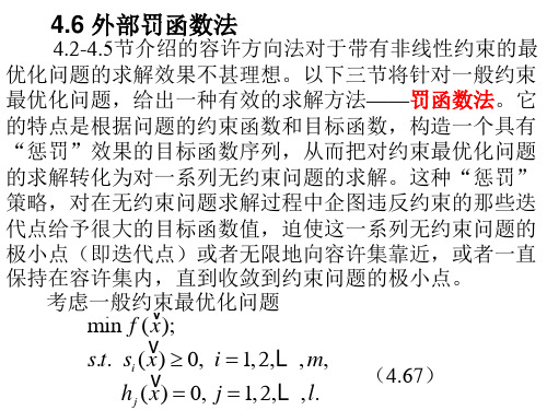
1. 算法的构成 首先讨论一个例子。求解
min x x ;
2 1 2 2
如图所示。此问题的容许集 D 是直线 x1 x2 2 。用 * T 图解法或Lagrange乘子法不难求出它的极小点是 x [1,1] 根据前面提出的惩罚策略,即 对容许点不予“惩罚”,而对非容 许点则给予正无穷大的“惩罚”, 设法将约束问题(4.68)转化为无约 束问题。 x2 x2 , x x 2 0
证 必要性是显然的。因为极小点是容许点。 充分性 设 x D ,这里的 D 是约束问题(4.67)
f ( x ) F ( x , ) [因 ( x ) 0] F ( x , ) [因x 是F的极小点] f ( x ). [因 ( x ) 0] 所以 x 也是约束问题(4.67)的极小点。 该定理说明,若由无约束问题(4.79)解出的极小点 x 属于(4.67)的容许集 D,则它就是约束问题(4.67)的 极小点。这时只需求解一次无约束问题。但实际上,这种 有利的情况很少发生,即 x 一般不属于 D。而若 x D , 则 x就一定不是约束问题(4.67)的极小点。这时,应该 增大 ,再重新求解无约束问题(4.79),新的极小点 将 向容许集进一步靠近,即向(4.67)的极小点进一步靠近。 把 在实际的算法中, 取为一个趋于正无穷大的正数 序列 k ,并对 k 0,1, 2, 依次求解无约束问题
最优潮流现代内点算法

优点: 具有二次收敛性 缺点: 1. 对不等式约束处理困难
2. 初始点必须在最优点附近才能保证算法的收敛性
3
三、现代内点算法
发展
1. 1949年Dantzig提出求解线性规划问题的单纯形法; 2. 1979年由Khachian提出第一个多项式时间算法——椭球法; 3. 1984年由Kmarmarkar提出了求解线性规划问题的新算法—— 现代内点算法。 4.1985年Gill证明了古典障碍函数法与 Kmarmarkar内点算法之间 存在着等价联系,从而将现代内点算法应用到非线性规划问题的 求解中。
7
三、现代内点算法
• 用牛顿法导出扰动KKT条件的修正方程为:
H xh(x) xg(x) xg(x)
Txh(x)
0
0
0
0 0
0x Lx 0y Ly
TTxxgg((xx))
0 0
0
0
0
0
0 0 L 0
0 0 0 U
I 0 Z 0
W 00I w uzlLLLLulwz
其中: H [ 2 x f( x ) 2 x h ( x )y 2 x g ( x )z (w )]
14
五、仿真结果
采用IEEE30系统进行仿真计算:
系统参数表:
系统 满阵
节点/线路 30/41
等式约束 60
不等式约束 121(3/6/30/82)
稀疏
30/41
60
140(14/15/29/82)
15
五、仿真结果
算法性能
16
对偶间隙
1.E+3
1.E+2
满阵
1.E+1
稀疏
斯坦福大学人工智能所有课程介绍
List of related AI Classes CS229covered a broad swath of topics in machine learning,compressed into a sin-gle quarter.Machine learning is a hugely inter-disciplinary topic,and there are many other sub-communities of AI working on related topics,or working on applying machine learning to different problems.Stanford has one of the best and broadest sets of AI courses of pretty much any university.It offers a wide range of classes,covering most of the scope of AI issues.Here are some some classes in which you can learn more about topics related to CS229:AI Overview•CS221(Aut):Artificial Intelligence:Principles and Techniques.Broad overview of AI and applications,including robotics,vision,NLP,search,Bayesian networks, and learning.Taught by Professor Andrew Ng.Robotics•CS223A(Win):Robotics from the perspective of building the robot and controlling it;focus on manipulation.Taught by Professor Oussama Khatib(who builds the big robots in the Robotics Lab).•CS225A(Spr):A lab course from the same perspective,taught by Professor Khatib.•CS225B(Aut):A lab course where you get to play around with making mobile robots navigate in the real world.Taught by Dr.Kurt Konolige(SRI).•CS277(Spr):Experimental Haptics.Teaches haptics programming and touch feedback in virtual reality.Taught by Professor Ken Salisbury,who works on robot design,haptic devices/teleoperation,robotic surgery,and more.•CS326A(Latombe):Motion planning.An algorithmic robot motion planning course,by Professor Jean-Claude Latombe,who(literally)wrote the book on the topic.Knowledge Representation&Reasoning•CS222(Win):Logical knowledge representation and reasoning.Taught by Profes-sor Yoav Shoham and Professor Johan van Benthem.•CS227(Spr):Algorithmic methods such as search,CSP,planning.Taught by Dr.Yorke-Smith(SRI).Probabilistic Methods•CS228(Win):Probabilistic models in AI.Bayesian networks,hidden Markov mod-els,and planning under uncertainty.Taught by Professor Daphne Koller,who works on computational biology,Bayes nets,learning,computational game theory, and more.1Perception&Understanding•CS223B(Win):Introduction to computer vision.Algorithms for processing and interpreting image or camera information.Taught by Professor Sebastian Thrun, who led the DARPA Grand Challenge/DARPA Urban Challenge teams,or Pro-fessor Jana Kosecka,who works on vision and robotics.•CS224S(Win):Speech recognition and synthesis.Algorithms for large vocabu-lary continuous speech recognition,text-to-speech,conversational dialogue agents.Taught by Professor Dan Jurafsky,who co-authored one of the two most-used textbooks on NLP.•CS224N(Spr):Natural language processing,including parsing,part of speech tagging,information extraction from text,and more.Taught by Professor Chris Manning,who co-authored the other of the two most-used textbooks on NLP.•CS224U(Win):Natural language understanding,including computational seman-tics and pragmatics,with application to question answering,summarization,and inference.Taught by Professors Dan Jurafsky and Chris Manning.Multi-agent systems•CS224M(Win):Multi-agent systems,including game theoretic foundations,de-signing systems that induce agents to coordinate,and multi-agent learning.Taught by Professor Yoav Shoham,who works on economic models of multi-agent interac-tions.•CS227B(Spr):General game playing.Reasoning and learning methods for playing any of a broad class of games.Taught by Professor Michael Genesereth,who works on computational logic,enterprise management and e-commerce.Convex Optimization•EE364A(Win):Convex Optimization.Convexity,duality,convex programs,inte-rior point methods,algorithms.Taught by Professor Stephen Boyd,who works on optimization and its application to engineering problems.AI Project courses•CS294B/CS294W(Win):STAIR(STanford AI Robot)project.Project course with no lectures.By drawing from machine learning and all other areas of AI, we’ll work on the challenge problem of building a general-purpose robot that can carry out home and office chores,such as tidying up a room,fetching items,and preparing meals.Taught by Professor Andrew Ng.2。
高斯牛顿法和内点法
高斯牛顿法和内点法高斯牛顿法与内点法是许多数值优化问题中常用的两种优化算法。
这两种方法有一些相似之处,但同时也存在一些显著的差异。
高斯牛顿法是一种用于解决非线性最小二乘问题的迭代算法。
该算法将待优化的目标函数拆解为一系列二次函数的和,然后通过不断优化每个二次函数的参数,最终获得目标函数最小值。
该算法主要用于解决大规模非线性回归问题。
该算法的迭代过程非常简单,每次迭代仅需要计算目标函数的梯度和海森矩阵,然后通过求解海森矩阵的逆矩阵来更新参数。
由于海森矩阵的逆矩阵通常比较难计算,因此该算法在实际应用中通常使用一些简单的近似方法来计算逆矩阵,例如拟牛顿法。
虽然高斯牛顿法非常高效,但是它也存在一些缺陷。
首先,该算法通常比较依赖初始参数,如果初始参数选取不好,可能会导致无法获得良好的最优解。
其次,该算法只能处理凸优化问题,对于非凸问题,可能会陷入局部最优解。
内点法是另一种常用的数值优化算法,该算法通常用于处理线性规划和二次规划问题。
该算法的基本思想是通过一系列迭代,将待求解的问题转化为逐步靠近可行解的新问题,并最终求解得到目标最小的最优解。
内点法的迭代过程非常复杂,每次迭代需要求解等式约束和不等式约束的牛顿方程组,并且需要保证迭代过程中所有的参数都满足约束条件。
与高斯牛顿法相比,内点法更加灵活,能够处理非凸问题,并且不受初始参数的影响。
除了以上提到的差异,高斯牛顿法和内点法在一些其他方面也存在差异。
例如,高斯牛顿法通常需要计算目标函数的梯度和海森矩阵,而内点法则需要处理约束条件,这导致内点法的计算复杂度更高。
此外,内点法还需要使用一些特殊的数据结构来处理问题,例如Klee-Minty方案和扰动技巧,这也增加了实现和调试的难度。
综上所述,高斯牛顿法和内点法都是常用的数值优化算法,在不同的问题中具有不同的优缺点。
选择正确的算法并根据具体的问题进行优化,是提高求解效率和精度的关键。
随着计算机硬件和算法的不断进步,数值优化将会在越来越多的领域发挥重要的作用。
凸优化、半定规划相关Matlab工具包总结(部分为C C++)
SoftwareFor some codes a benchmark on problems from SDPLIB is available at Arizona State University.∙CSDP 4.9, by Brian Borchers (report 1998, report 2001). He also maintains a problem library, SDPLIB.∙CVX, version 1.1, by M. Grant and S. Boyd.Matlab software for disciplined convex programming.∙DSDP 5.6 , by S. J. Benson and Y. Ye, parallel dual-scaling interior point code in C (manual); source and excutables available fromBenson's homepages.∙GloptiPoly3, by D. Henrion, J.-B. Lasserre and J. Loefberg;a Matlab/SeDuMi add-on for LMI-relaxations of minimization problemsover multivariable polynomial functions subject to polynomial or integer constraints.∙LMITOOL-2.0 of the Optimization and Control Group at ENSTA.∙MAXDET, by Shao-po Wu, L. Vandenberghe, and S. Boyd. Software for determinant maximization. (see also rmd)∙NCSOStools, by K. Cafuta, I. Klep, and J. Povh. An open source Matlab toolbox for symbolic computation with polynomials in noncommutingvariables, to be used in combination with sdp solvers.∙PENNON-1.1 by M. Kocvara and M. Stingl. It implements a penalty method for (large-scale, sparse) nonlinear and semidefiniteprogramming (see their report), and is based on the PBM method ofBen-Tal and Zibulevsky.∙PENSDP v2.0 and PENBMI v2.0, by TOMLAB Optimization Inc., a MATLAB interface for PENNON.∙rmd , by the Geometry of Lattices and Algorithms group at University of Magdeburg, for making solutions of MAXDET rigorous byapproximating primal and dual solution by rationals and testing forfeasibility.∙SBmethod (Version 1.1.3), by C. Helmberg. A C++ implementation of the spectral bundle method for eigenvalue optimization.∙SDLS by D. Henrion and J. Malick.Matlab package for solving least-squares problems over convexsymmetric cones.∙SDPA (version 7.1.2), initiated by the group around Masakazu Kojima.∙SDPHA does not seem to be available any more (it was package by F.A. Potra, R. Sheng, and N. Brixius for use with MATLAB).∙SDPLR (version 1.02, May 2005) by Sam Burer, a C package for solving large-scale semidefinite programming problems.∙SDPpack is no longer supported, but still available. Version 0.9 BETA, by F. Alizadeh, J.-P. Haeberly, M. V. Nayakkankuppam, M. L. Overton, and S. Schmieta, for use with MATLAB.∙SDPSOL (version beta), by Shao-po Wu & Stephen Boyd (May 20, 1996). A parser/solver for SDP and MAXDET problems with matrixstructure.∙SDPT3 (version 4.0), high quality MATLAB package by K.C. Toh, M.J.Todd, and R.H. Tütüncü. See the optimization online reference.∙SeDuMi, a high quality package with MATLAB interface for solving optimization problems over self-dual homogeneous cones started byJos F. Sturm.Now also available: SeDuMi Interface 1.04 by Dimitri Peaucelle.∙SOSTOOLS, by S. Prajna, A. Papachristodoulou, and P. A. Parrilo. A SEDUMI based MATLAB toolbox for formulating and solving sums ofsquares (SOS) optimization programs(also available at Caltech).∙SP (version 1.1), by L. Vandenberghe, Stephen Boyd, and Brien Alkire.Software for Semidefinite Programming.∙SparseCoLO, by the group of M. Kojima, a matlab package for conversion methods for LMIs having sparse chordal graph structure,see the Research report B-453.∙SparsePOP, by H. Waki, S. Kim, M. Kojima and M. Muramatsu, is a MATLAB implementation of a sparse semidefinite programmingrelaxation method proposed for polynomial optimization problems.∙VSDP: Verified SemiDefinite Programmin, by Christian Jansson.MATLAB software package for computing verified results ofsemidefinite programming problems. See the optimization onlinereference.∙YALMIP, free MATLAB Toolbox by J. Löfberg for rapid optmization modeling with support for, e.g., conic programming, integerprogramming, bilinear optmization, moment optmization and sum ofsquares. Interfaces about 20 solvers, including most modern SDPsolvers.Reports on software:∙M. Yamashita, K. Fujisawa, M. Fukuda, K. Nakata and M. Nakata."Parallel solver for semidefinite programming problem having sparseSchur complement matrix",Research Report B-463, Dept. of Math. and Comp. Sciences, TokyoInstitute of Technology, Oh-Okayama, Meguro, Tokyo 152-8552,September 2010.opt-online∙Hans D. Mittelmann."The state-of-the-art in conic optimization software",Arizona State University, August 2010, written for the "Handbook ofSemidefinite, Cone and Polynomial Optimization: Theory, Algorithms, Software and Applications".opt-online∙K.-C. Toh, M. J. Todd, and R. H. Tütüncü."On the implementation and usage of SDPT3 -- a Matlab softwarepackage for semidefinite-quadratic-linear programming, version 4.0", Preprint, National University of Singapore, June, 2010.opt-online∙K. Cafuta, I. Klep and J. Povh."NCSOSTOOLS: A Computer Algebra System for Symbolic andNumerical Computation with Noncommutative Polynomials",University of Ljubljana, Faculty of Mathematics and Physics, Slovenia, May 2010.opt-online∙I. D. Ivanov and E. De Klerk."Parallel implementation of a semidefinite programming solver based on CSDP on a distributed memory cluster",Optimization Methods and Software, Volume 25, Issue 3 June 2010 , pages 405 - 420 .OMS∙M. Yamashita, K. Fujisawa, K. Nakata, M. Nakata, M. Fukuda, K.Kobayashi and Kazushige Goto."A high-performance software package for semidefinite programs:SDPA 7",Department of Mathematical and Computing Sciences, Tokyo Institute of Technology, January, 2010.opt-online∙Sunyoung Kim, Masakazu Kojima, Hayato Waki and Makoto Yamashita."SFSDP: a Sparse Version of Full SemiDefinite ProgrammingRelaxation for Sensor Network Localization Problems",Report B-457, Dept. of Mathematical and Computing Sciences, Tokyo Institute of Technology, July 2009.opt-online∙K. Fujisawa, S. Kim, M. Kojima, Y. Okamoto and M. Yamashita."ser's Manual for SparseCoLO: Conversion Methods for SparseConic-form Linear Optimization Problems",Research report B-453, Department of Mathematical and Computing Sciences, Tokyo Institute of Technology, 2-12-1 Oh-Okayama,Meguro-ku, Tokyo 152-8552 Japan, February 2009.opt-online∙Sunyoung Kim, Masakazu Kojima, Martin Mevissen, Makoto Yamashita."Exploiting Sparsity in Linear and Nonlinear Matrix Inequalities viaPositive Semidefinite Matrix Completion",Research Report B-452, Department of Mathematical and ComputingSciences, Tokyo Institute of Technology, Oh-Okayama, Meguro, Tokyo 152-8552, Japan, November 2008.opt-online∙ D. Henrion, J. B. Lasserre, and J. Löfberg."GloptiPoly 3: moments, optimization and semidefinite programming", LAAS-CNRS, University of Toulouse, 2007.opt-online∙Didier Henrion and J茅r么me Malick."SDLS: a Matlab package for solving conic least-squares problems", LAAS-CNRS, University of Toulouse, 2007.opt-online∙M. Grant and S. Boyd."Graph Implementations for Nonsmooth Convex Programs",Stanford University, 2007.opt-online∙K. K. Sivaramakrishnan."A PARALLEL interior point decomposition algorithm for block-angular semidefinite programs",Technical Report, Department of Mathematics, North Carolina State University, Raleigh, NC, 27695, December 2006. Revised in June 2007 and August 2007.opt-online∙Makoto Yamashita, Katsuki Fujisawa, Mituhiro Fukuda, Masakazu Kojima, Kazuhide Nakata."Parallel Primal-Dual Interior-Point Methods for SemiDefinite Programs", Research Report B-415, Tokyo Institute of Technology, 2-12-1,Oh-okayama, Meguro-ku, Tokyo, Japan, March 2005.opt-online∙ B. Borchers and J. Young."How Far Can We Go With Primal-Dual Interior Point Methods forSDP?",New Mexico Tech, February 2005.opt-online∙H. Waki, S. Kim, M. Kojima and M. Muramatsu."SparsePOP : a Sparse Semidefinite Programming Relaxation ofPolynomial Optimization Problems",Research Report B-414, Dept. of Mathematical and ComputingSciences, Tokyo Institute of Technology, Oh-Okayama, Meguro152-8552, Tokyo, Japan, March 2005.opt-online∙M. Kocvara and M. Stingl."PENNON: A code for convex nonlinear and semidefinite programming", Optimization Methods and Software (OMS), Volume 18, Number 3,317-333, June 2003.∙Brian Borchers."CSDP 4.0 User's Guide",user's guide, New Mexico Tech, Socorro, NM 87801, 2002.opt-online∙M. Yamashita, K. Fujisawa, and M. Kojima."SDPARA : SemiDefinite Programming Algorithm PARAllel Version", Parallel Computing Vol.29 (8) 1053-1067 (2003).opt-online∙J. Sturm."Implementation of Interior Point Methods for Mixed Semidefinite and Second Order Cone Optimization Problems",Optimization Methods and Software, Volume 17, Number 6, 1105-1154, December 2002.optimization-online∙S. Benson and Y. Ye."DSDP4 Software User Guide",ANL/MCS-TM-248; Mathematics and Computer Science Division;Argonne National Laboratory; Argonne, IL; March 2002.opt-online∙S. Benson."Parallel Computing on Semidefinite Programs",Preprint ANL/MCS-P939-0302; Mathematics and Computer Science Division Argonne National Laboratory 9700 S. Cass Avenue Argonne, IL, 60439; March 2002.opt-online∙ D. Henrion and J. B. Lasserre."GloptiPoly - Global Optimization over Polynomials with Matlab andSeDuMi",LAAS-CNRS Research Report, February 2002.opt-online∙M. Kocvara and M. Stingl."PENNON - A Generalized Augmented Lagrangian Method forSemidefinite Programming",Research Report 286, Institute of Applied Mathematics, University of Erlangen, 2001.opt-online∙ D. Peaucelle, D. Henrion, and Y. Labit."User's Guide for SeDuMi Interface 1.01", Technical report number01445 LAAS-CNRS : 7 av. du Colonel Roche, 31077 Toulouse Cedex 4, FRANCE November 2001.opt-online∙Jos F. Sturm."Using SEDUMI 1.02, a MATLAB Toolbox for Optimization OverSymmetric Cones (Updated for Version 1.05)",October 2001.opt-online∙Hans D. Mittelmann."An Independent Benchmarking of SDP and SOCP Solvers",Technical Report, Dept. of Mathematics, Arizona State University, July2001.opt-online∙K. Fujisawa, M. Fukuda, M. Kojima and K. Nakata."Numerical Evaluation of SDPA",Research Report B-330, Department of Mathematical and ComputingSciences, Tokyo Institute of Technology, Oh-Okayama, Meguro-ku,Tokyo 152, September 1997.ps.Z-file (ftp) or dvi.Z-file (ftp)∙L. Mosheyev and M. Zibulevsky."Penalty/Barrier Multiplier Algorithm for Semidefinite Programming:Dual Bounds and Implementation",Research Report #1/96, Optimization Laboratory, Technion, November 1996.ps-file (http)Due to several requests I have asked G. Rinaldi for permission to put his graph generator on this page. Here it is: rudy (tar.gz-file)Last modified: Tue Oct 26 15:10:14 CEST 2010。
线性规划karmarkar方法的初始内点的求法
线性规划karmarkar方法的初始内点的求法线性规划Karmarkar方法是一种最优化算法,可以求解线性规划问题。
它于1984年由Karmarkar发表,被认为是一种重大突破。
Karmarkar方法以全局优化作为目标,建立了一种计算最优解的新方法。
通过求解初始内点,Karmarkar方法可以有效地求解线性规划问题。
二、定义Karmarkar方法是一种基于内点求解线性规划问题的algorithm。
点Interior Point)是指在一个满足线性不等式约束条件的线性函数的极值的计算过程中,其可行解区域内的一个点,这个点不在可行解变量的边界上。
其定义为:若存在矩阵A,则内点x*称为可行解(满足线性不等式约束条件)下的点,在它以及它周围的某一范围内,使得函数f(x)取极值,且满足所有线性不等式约束条件。
三、Karmarkar算法概述Karmarkar算法是一种基于内点的求解线性规划问题的algorithm,旨在求解满足线性不等式约束条件的线性函数的极值。
这种方法的目的是从满足线性不等式约束的潜在可行解空间中找出最优解。
Karmarkar算法以一系列的步骤来计算线性规划问题的最优解:首先,从初始解开始,将其与约束条件合并,然后计算该解的函数值,称为函数值分析;接着,在函数值分析的步骤中,对该初始内点进行增强,直到找到最优解为止。
四、Karmarkar算法的求解步骤1.解基本解:从原始问题中计算出一个可行解,称为基本解,是一个向量,它满足和所有线性不等式约束条件。
2.择初始内点:找出一个可行解,该解与基本解最接近,但不位于边界上,称为初始内点。
3.数值分析:以初始内点为基础,计算函数的函数值,然后通过改变内点来调整目标函数的值。
4.索步骤:将更新的内点和上述等式约束条件作为入口,搜索步骤将会求解最优解。
五、实例下面我们来看一个简单的例子。
约束条件为:Ax b求解的目标是: min f(x) = cTx首先,我们确定基本解: x_0 = (3,1,2)初始内点: x* = (2.5,0.5,1.5)此时,函数值为: f(x*) =10接下来,我们使用函数值分析方法,以计算出最优解。
线性规划的可行点算法
摘要本文研究的是线性规划的可行点算法,一个由线性规划的内点算法衍生而来的算法.线性规划的内点算法是一个在线性规划的可行域内部迭代前进的算法.有各种各样的内点算法,但所有的内点算法都有一个共同点,就是在解的迭代改进过程中,要保持所有迭代点在可行域的内部,不能到达边界.当内点算法中的迭代点到达边界时,现行解至少有一个分量取零值.根据线性规划的灵敏度分析理论,对线性规划问题的现行解的某些分量做轻微的扰动不会改变线性规划问题的最优解.故我们可以用一个很小的正数赋值于现行锯中等于零的分量,继续计算,就可以解出线陛规划问题的最优解.这种对内点算法的迭代点到达边界情况的处理就得到了线性规划的可行点算法.它是一个在可行域的内部迭代前进求得线性规划的最优解的算法.在此算法中,只要迭代点保持为可行点.本文具体以仿射尺度算法和原始一对偶内点算法为研究对象,考虑这两种算法中迭代点到达边界的情况,得到相对应的’仿射尺度可行点算法’和’原始.对偶可行点算法,.在用理论证明线性规划的可行点算法的可行性的同时,我们还用数值实验验正了可行点算法在实际计算中的可行性和计算效果.关键词:线性规划,仿射尺度算法,原始一对偶内点算法,内点,可行点算法,步长可行点.AbstractderivedThisDaperfocusesonafeasiblepointalgorithmforlinearprogramming,analgorithmfromtheinteriorpointalgorithmsforlineza"programming.TheinteriorpointalgorithmsfindtheoptimalsolutionofthelinearprogrammingbysearchingwithinthefeasmleTe譬ionofthelinearprogramming.ThereareaUkindsofinteriorpointalgorithlrmalltheforlinearprogramnfing.Butalltheseinteriorpointalgorithmsshareaspeciality,whichissolution|terativeDointscannotreachtheboundsAccordingtothesensitivitytheory,theoptimalofthelinearprogrammingwillnotbechangedbylittledisturbancesofthepresentsolution·SoWeletthe{xjIzJ=o,J=1,2,-··)n)equalaverysmallpositivenunlber,goonwiththecomputatio“一andthenwegettheoptimalsolutionofthelinearprogramming.Alltheseleadtothedevelopment。
- 1、下载文档前请自行甄别文档内容的完整性,平台不提供额外的编辑、内容补充、找答案等附加服务。
- 2、"仅部分预览"的文档,不可在线预览部分如存在完整性等问题,可反馈申请退款(可完整预览的文档不适用该条件!)。
- 3、如文档侵犯您的权益,请联系客服反馈,我们会尽快为您处理(人工客服工作时间:9:00-18:30)。
Examples
inequality form LP (m = 100 inequalities, n = 50 variables)
102 140
Newton iterations
duality gap
10
0
120 100 80 60 40 20 0 0 40 80 120 160 200
T T ⋆
c
i = 1, . . . , 6
x
⋆
x⋆(10)
hyperplane c x = c x (t) is tangent to level curve of φ through x⋆(t)
Interior-point methods 12–6
Dual points on central path
Interior-point methods 12–11
Convergence analysis
number of outer (centering) iterations: exactly log(m/(ǫt(0))) log µ plus the initial centering step (to compute x⋆(t(0))) centering problem minimize tf0(x) + φ(x) see convergence analysis of Newton’s method • tf0 + φ must have closed sublevel sets for t ≥ t(0) • classical analysis requires strong convexity, Lipschitz condition • analysis via self-concordance requires self-concordance of tf0 + φ
Interior-point methods
m i=1 log(−fi (x)) 10 5 0 −5 −3
−2
−1
u
0
1
12–4
logarithmic barrier function
m
φ ( x) = −
i=1
log(−fi(x)),
dom φ = {x | f1(x) < 0, . . . , fm(x) < 0}
m m i=1 log(−fi (x))
F0(x⋆(t)) +
i=1
Fi(x⋆(t)) = 0
Interior-point methods
12–9
example
minimize cT x subject to aT i x ≤ bi ,
i = 1, . . . , m
• objective force field is constant: F0(x) = −tc • constraint force field decays as inverse distance to constraint hyperplane: Fi(x) = −ai , T bi − a i x Fi(x)
m
∇f 0 ( x ) +
i=1
λ i ∇ f i ( x ) + AT ν = 0
difference with KKT is that condition 3 replaces λifi(x) = 0
Interior-point methods
12–8
Force field interpretation
Convex Optimization — Boyd & Vandenberghe
12. Interior-point methods
• inequality constrained minimization • logarithmic barrier function and central path • barrier method • feasibility and phase I methods • complexity analysis via self-concordance • generalized inequalities
m m m
Interior-point methods
12–5
Central path
• for t > 0, define x⋆(t) as the solution of minimize tf0(x) + φ(x) subject to Ax = b (for now, assume x⋆(t) exists and is unique for each t > 0) • central path is {x⋆(t) | t > 0} example: central path for an LP minimize cT x subject to aT i x ≤ bi ,
12–1
Inequality constrained minimization
minimize f0(x) subject to fi(x) ≤ 0, Ax = b
i = 1, . . . , m
(1)
• fi convex, twice continuously differentiable • A ∈ Rp×n with rank A = p • we assume p⋆ is finite and attained • we assume problem is strictly feasible: there exists x ˜ with x ˜ ∈ dom f0, fi(˜ x ) < 0, i = 1, . . . , m, Ax ˜=b
hence, strong duality holds and dual optimum is attained
Interior-point methods
12–2
Examples
• LP, QP, QCQP, GP • entropy maximization with linear inequality constraints minimize i=1 xi log xi subject to F x g Ax = b with dom f0 = Rn ++ • differentiability may require reformulating the problem, e.g., piecewise-linear minimization or ℓ∞-norm approximation via LP • SDPs and SOCPs are better handled as problems with generalized inequalities (see later)
Interior-point methods 12–3
n
Logarithmic barrier
reformulation of (1) via indicator function: minimize f0(x) + subject to Ax = b
m i=1 I− (fi (x))
where I−(u) = 0 if u ≤ 0, I−(u) = ∞ otherwise (indicator function of R−) approximation via logarithmic barrier minimize f0(x) − (1/t) subject to Ax = b • an equality constrained problem • for t > 0, −(1/t) log(−u) is a smooth approximation of I− • approximation improves as t → ∞
2
=
1 dist(x, Hi)
where Hi = {x | aT i x = bi }
−c − 3c t=1
Interior-point methods
t=3
12–10Hale Waihona Puke Barrier method
given strictly feasible x, t := t(0) > 0, µ > 1, tolerance ǫ > 0. repeat 1. 2. 3. 4. Centering step. Compute x⋆(t) by minimizing tf0 + φ, subject to Ax = b. Update. x := x⋆(t). Stopping criterion. quit if m/t < ǫ. Increase t. t := µt.
i=1
⋆ T λ⋆ ( t ) f ( x ) + ν ( t ) (Ax − b) i i
• this confirms the intuitive idea that f0(x⋆(t)) → p⋆ if t → ∞: p⋆ ≥ g (λ⋆(t), ν ⋆(t)) = L(x⋆(t), λ⋆(t), ν ⋆(t))
• convex (follows from composition rules) • twice continuously differentiable, with derivatives ∇φ ( x ) = ∇2 φ ( x ) = 1 ∇f i ( x ) − f ( x ) i i=1 1 1 2 T ∇ f ( x ) ∇ f ( x ) + ∇ fi ( x) i i 2 f ( x) − fi ( x) i=1 i=1 i
⋆ ⋆ where we define λ⋆ i (t) = 1/(−tfi (x (t)) and ν (t) = w/t