调制传递函数和调制传递函数曲线
mtf调制传递函数
mtf调制传递函数MTF (Modulation Transfer Function) refers to the ability of an imaging system to faithfully reproduce details of an object, such as contrast and spatial resolution. The MTF describes the system's ability to transfer contrast at different spatial frequencies from the object to the image. In this article, wewill discuss the MTF modulation transfer function in detail.The MTF modulation transfer function is a measurement of the system's spatial frequency response. It represents the abilityof the system to transfer contrast from the object to the image. The MTF is typically represented as a graph, with contrastplotted against spatial frequency.The MTF is derived from the sine wave response of the system.A sine wave of a specific spatial frequency is projected ontothe system, and the resulting image is analyzed for contrast.The contrast of the image is then normalized against thecontrast of the original sine wave to obtain the MTF value.The MTF is influenced by various factors, including lens quality, sensor resolution, and image processing algorithms. Higher quality lenses and sensors generally result in higher MTF values, indicating better contrast transfer. Similarly, advanced image processing algorithms can enhance the MTF by reducingnoise and sharpening details.The MTF is often used as a measure of image quality in various fields, including photography, microscopy, and medical imaging. With a higher MTF, the resulting images will havebetter contrast and sharper details, leading to improved image quality and diagnostic accuracy.The MTF is typically measured at various spatial frequencies, ranging from low to high. The MTF graph shows how the system's contrast transfer changes with increasing spatial frequency. A perfect system would have an MTF of 1 at all spatial frequencies, indicating perfect contrast transfer. However, in real-world systems, the MTF gradually decreases with increasing spatial frequency.The MTF graph can provide valuable information about the performance of an imaging system. For example, the spatial frequency at which the MTF drops to a certain value, such as 0.5, is often used as a measure of spatial resolution. A higherspatial resolution indicates that the system can reproducedetails with higher frequency.In conclusion, the MTF modulation transfer function is a crucial measure of image quality. It quantifies the system's ability to transfer contrast at different spatial frequencies.By measuring and analyzing the MTF, one can assess the performance of an imaging system and understand its capabilityto reproduce fine details. With a higher MTF, the system canproduce images with better contrast and spatial resolution, leading to improved image quality and accuracy in various applications.。
详细解读MTF成像曲线图
正弦光栅
国
中 我们再回过头来看反差。反差 =(照度的最大值 - 照度的最小值)/(照
度的最大值 + 照度的最小值)。所以,反差的数值总是小于等于 1 的。 这里我们引入调制度 M 的概念 :
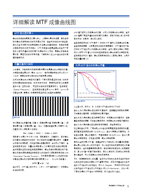
它的衰减过程很慢,说明其素质还是不错的。 曲线 B 所代表的镜头在低频表现很好,说明镜头的反差很好,但随 着空间频率的提高,它的曲线衰减很快,说明镜头的分辨率不算很好。 曲线 C 所代表的镜头在低频时就很快衰减,综合素质较低。 和上面的曲线不同,厂商绘制 MTF 曲线时都是固定空间频率和光圈。
测量反差与分辨率
利用 MTF 曲线判断镜头质量
众所周知,对数码照片成像素质影响最大的是镜头的分辨率和反差。
பைடு நூலகம்
分辨率的单位是线对 / 毫米(lp/mm),相邻的黑白两条线可以称为一 个线对,每毫米能够分辨出的线对数就是分辨率。
如何测试镜头的分辨率和反差呢?厂商利用拍摄正弦光栅(测试标 板中的黑白相间的栅格)的方法进行测试,亮度按正弦变化的周期 图形叫做“ 正弦 光栅”。 而正弦 光栅的 疏密 程 度 被 称为“ 空间频 率”
MTF 曲线与横 轴、 纵轴 所围成的空间, 面 积 越 大 越 好。
1 2
社 MTF 曲线越平直越好,平直性说明镜头边缘和中心部分的
成像均匀性 S 曲线与 M 曲线越接近越好
3
版 低频(10LP/mm)曲线代表镜头的反差特性,高频(30LP/
mm)曲线代表镜头的分辨率特性
出不要将不同焦距段、不同档次、不同规格(全幅、APS-C 画幅)以及定焦和变焦等不同镜头的 MTF 图进行比较, 4 因为它们的特性受设计规格、光学特性、像差以及成本、
其中固定空间频率低频(10 线对 /mm)曲线代表镜头反差特性,这 条曲线越高,镜头反差越大。而固定高频(30 线对 /mm)曲线代表 镜头分辨率特性,这条曲线越高,镜头分辨率越高。
光信息存储

访问时间可以做到在200毫秒以下。
一、光全息存储关键技术及原理
双色记录
全息数据记录的设备在双色全息记录的过程中, 参考光和信号光固定使用一个特殊的波长(绿光、 红光、甚至红外光),而敏化光束为一个单独的短 波长激光(蓝光或者紫外光)。敏化光束用来使材 料在记录过程之前和之后变得敏感,而信息将通过 参考光和信号光在晶体中记录下来。在读取的过程 中,仍然通过单独照射参考光来实现,由于参考光 波长较长,它无法在使被束缚的电子在读取阶段激 发,因此需要短波长的敏化光来擦除记录的信息。
关于光全息存储的探讨
光信息1001 唐丽红
目录
一、光全息存储关键技术及原 理 二、光全息存储的性能表征 三、光全息存储材料 四、光全息存储应用前景
光全息存储的提出
1984年, DennisGabor在 为提高电子显微镜 的分辨率时提出 1991年, 光驱问世; 1993年,第二代 MPC规格问世 1995年夏, Multimdeia PCWork ing Group公布第三代 规格标准,光驱速度提 高到四倍速。
全息光存储 的巨大竞争 力体现在它 所具有的超 大存储容量、 超高存储密 度和越快的 存取速度等 方面。 Inphase公 司和 Optware公 司已经在这 一领域中迈 出了坚实的 步伐,取得 了令人瞩目 的成就
1
2 2
3
参考文献
[1]景敏.全息显示技术发展与现状.[J].科 技广场.2008(7),232-234 [2]刘玉照.激光全息存储技术的发展.[J]. 情报科55学,2000(18),473-475 [3]江涛.信息存储新领域——全息存储及 其材料.[J].信息记录材料.2006(7),32-35
一、光全息存储关键技术及原理
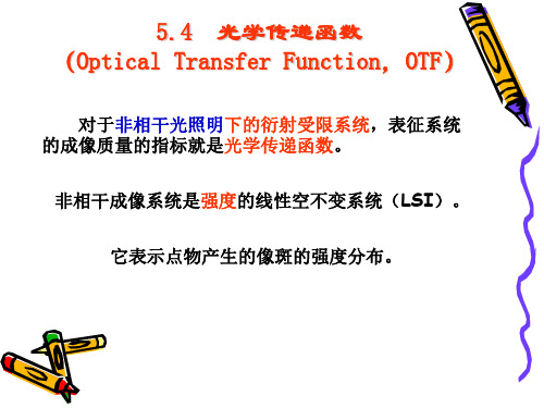
5.4 光学传递函数(OTF)
f ( x , y ) = aL{ f ( x , y )}
Ig
物 经过成像系统 像
Ii
x0
I g (~0 , ~0 ) = a + b cos 2π (ξ 0 ~0 ,η 0 ~0 ) + ϕ g (ξ 0 ,η 0 ) x y x y
xi
[
]
I i ( x i , yi ) = a + bM cos 2π (ξ 0 x i ,η 0 yi ) + ϕ g (ξ ,η ) + ϕ (ξ ,η )
它表示点物产生的像斑的强度分布。 它表示点物产生的像斑的强度分布。
非相干光照明下, 一. 非相干光照明下,衍射受限系统的成像规律 1. 物像关系(空域中) 物像关系(空域中)
~ y ~ I i ( x i , yi ) = k ∫∫ I g ( x0 , ~0 )hI ( x i − x0 , yi − ~0 )dx0 d~0 y ~ y = kI g ( x i , yi ) ∗ hI ( x i , yi )
Vi =
(a + bM (ξ ,η )) − (a − bM (ξ ,η )) b M (ξ ,η ) = (a + bM (ξ ,η )) + (a − bM (ξ ,η )) a
说明对比度下降了! 说明对比度下降了! 表明产生了条纹错开! 表明产生了条纹错开!
综合上式, 综合上式,有
Vi = V g M (ξ ,η )
,有
i i
∫∫ P ( x , y )P ( x + λd ξ , y + λd η )dxdy Η (ξ ,η ) = ∫∫ P ( x , y ) dαdβ ∫∫ P ( x , y )P ( x + λd ξ , y + λd η )dxdy = ∫∫ P ( x, y )dαdβ
CCD光子转移曲线及调制传递函数参数测试技术的实现

电工技术|2016年4月下|233CCD 光子转移曲线及调制传递函数参数测试技术的实现李 金 陈红兵中国电子科技集团公司第44研究所,重庆 400060摘要:研究列举了评价电荷耦合器件(CCD )光电性能的主要参数,详细介绍了光子转移曲线和调制传递函数参数测试方法和所需的测试设备条件及实现参数测试的过程。
关键词:电荷耦合器件;光子转移曲线;调制传递函数;测试方法 中图分类号:TN386.5文献标识码:A文章编号:1002-1388(2016)04-0233-03CCD 在中国军用和民用领域的用途越来越广泛,发挥着重要作用,CCD 光电性能参数测试及时反馈CCD 器件的性能参数状态,配合CCD 研制的顺利进行,是器件研制过程中的重要一环。
CCD 光电性能参数测试技术包括测试方法和测试系统两部分,建立测试系统首先要进行测试方法的研究,掌握各个被测参数的测试条件、测试仪器、测试过程和计算方法。
选择更适合的测试方法来搭建测试平台,建立测试系统。
CCD 包含的光电性能参数指标主要有:电荷-电压转换因子、电荷转移效率、暗信号、暗信号非均匀性(固定图像噪声)、读出噪声、光响应非线性、饱和输出信号、动态范围、信噪比、缺陷、光响应非均匀性、响应率、量子效率、光谱响应范围、调制传递函数、对比度传递函数、满阱电荷。
一些常规的参数如饱和电压、响应非均匀性、暗信号、动态范围等,测试方法比较简单易理解,下面重点介绍一下光子转移曲线(电荷-电压转换因子CVF )和调制传递函数MTF 的测试方法。
光子转移曲线可以全面的表征CCD 器件的综合性能,调制传递函数是评价CCD 器件成像性能的重要指标。
1 电荷-电压转换因子测试方法(光子转移曲线法)光子转移曲线[1]最重要的作用是表征CCD 处于最佳性能和最优工作状态。
光子转移方法可以用于估计众多的CCD 器件参数,这些参数包括读出噪声,暗电流,量子效率,满阱电荷,响应非线性,响应非均匀性,灵敏度,信噪比,动态范围等。
ZEMAX 中的调制传递函数MTF衍射极限是如何计算的?
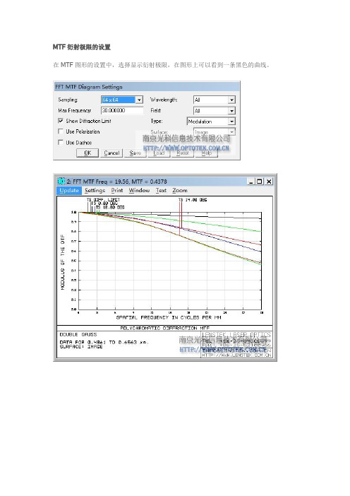
在MTF图形的设置中,选择显示衍射极限,在图形上可以看到一条黑色的曲线。
针对Focal 和Afocal两种模式,ZEMAX针对衍射极限的计算说名如下:
有以上信息可知,衍射极限由1.22 *λ *F# 决定。
其中λ 为波长,F# 就是我们要讨论的,因为在系统中有好几种F#
Image space F/# - 像空间F/#
Image space F/# is the ratio of the paraxial effective focal length calculated at infinite conjugates over the paraxial entrance pupil diameter. Note that infinite conjugates are used to define this quantity even if the lens is not used at infinite conjugates.
由以上信息可知:像空间F#是系统的有效焦距与入瞳直径的比值,而这两个参数都是以近轴光学为基础的。
而且,这种F#不会因为共轭状态的改变而有任何变化,很显然,MTF 的衍射极限不会以此为准。
近轴工作F/#及工作F/#
近轴工作F/#是以近轴的边缘光线在像空间的角度来计算F/#
工作F/#是以真实的边缘光线在像空间的角度来计算F/#,这个也就是我们的WFNO,其中这个就是计算MTF衍射极限的基础。
其中也要注意,系统计算的WFNO是以第一视场的边缘光学来进行计算的。
因此无论增加几个其他的视场,都不会影响ZEMAX计算的衍射极限。
CT成像质量影响因素及简易测试方法
CT成像质量影响因素及简易测试方法摘要:CT(Computed Tomography),指电子计算机断层扫描。
它是1967年由英国工程师Hounsfield发明,1972年开始应用于临床。
CT成像基本原理是相对均匀的X线束照射人体不同检查部位的组织、器官,因其密度、厚度等差别产生不同的衰减,导致探测器接收透过该层面的剩余X线量的不同,转变为不同强度的可见光后,由光电转换器转为电信号,再经模拟/数字转换器转为数字信号,输入计算机处理成不同的灰阶的相应的人体组织、器官的CT成像,当人体产生疾病后,其不同密度的病理组织同样能被CT设备所检出,这就是CT能够检出病变的基本原理。
由于CT的工作原理较为复杂,这就对放射科技师的技术要求要高,技师不仅要具备基本的控制CT扫描图像质量的方法,还要掌握多种行之有效的方式方法。
本文主要研究CT技师如何保证扫描图像的质量,并提出具体可行的方法。
关键词:CT;图像质量;方法随着经济的快速发展,医学水平不断提高,CT技术也不断地成熟。
如多排螺旋CT技术在临床诊断中的应用无论在扫描范围、成像速度、成像质量上都有显著的成果。
再如灌注CT技术和PET(正电子发射型计算机断层显像)/CT的不断发展使得CT扫描技术有了更为广泛的应用前景。
无论CT扫描成像的技术有多先进总会受到各种各样的因素干扰,影响成像质量,不利于医生的准确诊断。
所以CT成像质量有专业的评价标准。
1 CT图像质量评价标准1.1 空间分辨率空间分辨率是成像的量化指标,是用来衡量CT成像质量的一个重要参数。
一般情况下高对比度空间分辨率采用的是调制传递函数来描述,CT成像的调制传递函数和X射线焦点机检测器的孔径大小、重建算法有密切关系,与扫描物体大小和X射线量没有关系。
1.2 噪声噪声主要是指在ct扫描成像过程中亮度水平的波动。
噪声一般会在X射线光子发射过程中或者是吸收转化中出现,限制了系统的检测能力。
信号噪声在被重建算法滤波之后会以影像噪声的形式出现在CT图像上。
光学仪器概论第五章

第五章 光学系统的质量指标如何评价光学系统的光信息传递质量,即对非成像光学系统的光束传输质量怎样?成像光学系统的成像质量如何?一直是光学工作者极为重视且不断探讨的问题。
如对成像光学系统,传统的评价方法是星点法和分辨率法。
星点检验是观察点光源通过光学系统所得到的像斑形状。
光学系统没有几何像差时,像斑为标准的艾里圆,有几何像差或离焦时,光强分散。
光学系统有中心误差,装配应力或玻璃折射率不均匀等,均会使星点形状不对称或不规则。
但这种方法属主观检验,不同的观察者看法存在差别,是定性和半定量的,它的规定也只能是比较抽象和笼统的。
分辨率法比较简单、方便、意义明确,能够用数量表示。
但它只能表述细节能不能分辨的界限,对于较粗线条的成像质量,不能作出定量的评价,就是说,有两个物镜分辨率一样,但粗线条的明晰度可能不一样。
实际上是一个物镜质量好,一个较差,但分辨率法反映不出来。
此外,尚会出现为分辨情况,测出的分辨率可能比理论分辨率还高。
1900~1904年德国光学工作者哈德曼(Hartman )基于几何像差的概念,用米字形光阑模拟光线,测量除畸变、倍率色差外的其它五种几何像差。
其优点是§测量结果可直接与光线追踪结果相比较。
但它没考虑衍射,且测量工作量大。
此外还有阴影法、干涉法,它们比较适用于非成像光学系统,对于成像光学系统主要用于测量轴上点成象质量,测量范围受限制。
电视出现以后,同样涉及到像质评价问题。
从事电学行业的人和光学行业的人思维模式不同,他们将时域的问题扩展为空域,引入了空间频率的概念。
发现菲涅耳—基尔霍夫衍射积分公式如将积分域拓宽到无穷大恰为傅里叶变换式,从而出现了傅里叶光学,推动了现代光学的发展,这恰恰证明了交叉学科的碰撞出现了科学进步的火花。
对于像质评价则产生了光学传递函数法。
从而使像质评价更为客观、合理。
§ 5.1分辨率如前所述分辨率是以光学系统所能分辨开两垂轴靠近像点的能力为准。
- 1、下载文档前请自行甄别文档内容的完整性,平台不提供额外的编辑、内容补充、找答案等附加服务。
- 2、"仅部分预览"的文档,不可在线预览部分如存在完整性等问题,可反馈申请退款(可完整预览的文档不适用该条件!)。
- 3、如文档侵犯您的权益,请联系客服反馈,我们会尽快为您处理(人工客服工作时间:9:00-18:30)。
Modulation Transfer Function (MTF) and MTF Curves
MTF curves show resolution and contrast information simultaneously allowing a lens to be evaluated based on the requirements for a specific application and can be used to compare the performance of multiple lenses. Used correctly, MTF curves can help determine if an application is actually feasible. For information on how to read an MTF curve, seeLens Performance Curves. Figure 1 is an example of an MTF curve for a 12mm lens used on the Sony IXC 625 sensor, which has a sensor format of 2/3" and 3.45μm pixels. The curve shows lens contrast over a frequency range from 0 lp/mm to 150 lp/mm (sensor’s limiting resolution is 145lp/mm). Additionally, this lens has its f/# set at 2.8 and is set at a PMAG of 0.05X, which yields a FOV of approximately 170mm for 20X the horizontal dimensions of the sensor. This FOV/PMAG will be used for all examples in this section. White light is used for the simulated light source.
Figure 1: MTF curve for a 12mm lens used on the Sony IXC 625 sensor. This curve provides a variety of information. The first thing to note is that the diffraction limit is represented by the black line. The black line indicates that the maximum theoretically possible contrast that can be achieved is almost 70% at the 150lp/mm frequency, and that no lens design, no matter how good, can perform higher than this. Additionally, there are three colored lines: blue, green, and red. These lines correspond to how this lens performs across the sensor in the center (blue), the 0.7X position at 70% of the full field on the sensor (green), and the corner of the sensor (red), respectively. It is clearly shown that at lower and higher frequencies contrast reproduction is not the same across the entire sensor and, thus, not the same over the FOV.
Additionally, it can be seen that there are two green and two red lines. These lines represent the tangential and sagittal contrast components associated with detail reproduction that is not in the center of the FOV. Due to aberrational effects, a lens will produce spots that are not completely round and will therefore have different sizes in the horizontal and vertical orientation. This size variation leads to spots blending together more quickly in one direction than the other, and produces different contrast levels in different axes at the same frequency. It is very import to consider the implications of the lower of these two values when evaluating a lens for a given application. It is generally advantageous to maximize the contrast level across the entire sensor to gain the highest levels of performance in a system.
COMPARING LENS DESIGNS AND CONFIGURATIONS Example 1: Comparison of two different lens designs with the same focal length (fl), 12mm, at f/2.8 Figure 2 examines two different lenses of the same focal length that have the same FOV, sensor, and f/#. These lenses will produce systems that are the same size but differ in performance. In analysis, the horizontal light blue line at 30% contrast on Figure 2a demonstrates that at least 30% contrast is achievable essentially everywhere within the FOV, which will allow for the entire capability of the sensor to be well-utilized. For Figure 2b, nearly half the field is below 30% contrast. This means that better image quality will only be achievable at half of the sensor. Also to note, the orange box on both curves represents the intercept frequency of the lower performance lens in Figure 2b with 70% contrast. When that same box is placed on Figure 2a, tremendous performance difference can be seen even at lower frequencies between the two lenses.
The difference between these lenses is the cost associated with overcoming both design constraints and fabrication variations; Figure 2a is associated with a much more complex design and tighter manufacturing tolerances. Figure 2a will excel in both lower resolution and demanding resolution applications where relatively short working distances for larger field of view are required. Figure 2b will work best where more pixels are needed to enhance the fidelity of image processing algorithms and where lower cost is required. Both lenses have situations where they are the correct choice, depending on the application.