Field Calculator 的使用
使用ArcGIS统计栅格数据面积
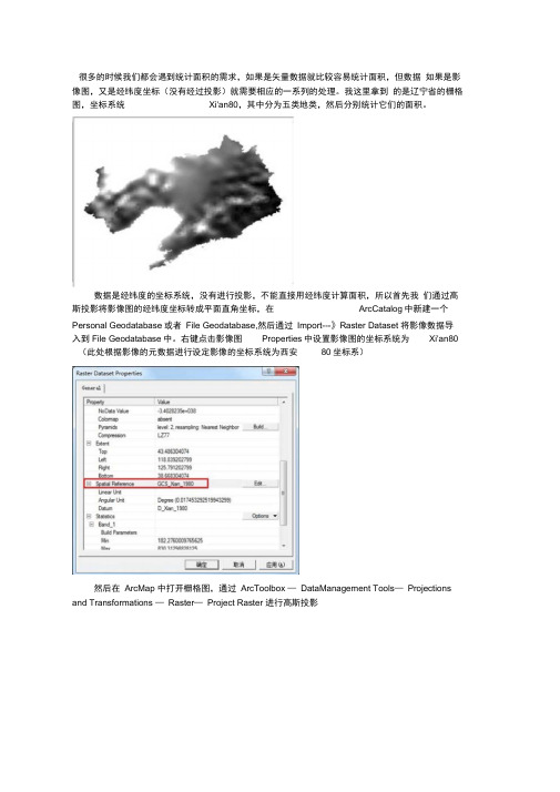
很多的时候我们都会遇到统计面积的需求,如果是矢量数据就比较容易统计面积,但数据如果是影像图,又是经纬度坐标(没有经过投影)就需要相应的一系列的处理。
我这里拿到的是辽宁省的栅格图,坐标系统Xi'an80,其中分为五类地类,然后分别统计它们的面积。
数据是经纬度的坐标系统,没有进行投影,不能直接用经纬度计算面积,所以首先我们通过高斯投影将影像图的经纬度坐标转成平面直角坐标,在ArcCatalog中新建一个Personal Geodatabase或者File Geodatabase,然后通过Import---》Raster Dataset 将影像数据导入到File Geodatabase中。
右键点击影像图Properties中设置影像图的坐标系统为Xi'an80 (此处根据影像的元数据进行设定影像的坐标系统为西安80坐标系)然后在ArcMap 中打开栅格图,通过ArcToolbox —DataManagement Tools—Projections and Transformations —Raster—Project Raster 进行高斯投影投影之后,就可以进行分类计算了,将投影后的影像图通过栅格分析工具进行重分类, 选择Spatial Analyst工具栏下拉菜单的"Reclassify ••”项Spatial AnalystSpatial Analyst ▼La吟:lExtCSOBjOOSpl 二J 務L L distanceDensity...Interpola te to RasterSurface AnalysisCell Statistics...Neighborhood Statistics.,,Zonal Statistics-Zonal Histogram在重分类后的影像上点击鼠标右键,选择" Open Attribute Table Reclassify.«.Rastsr Calculator*其中COUNT字段中的数值时代表每类地物中所包含的像素个数,这样的话我们就可以通过像素个数*每个像素的面积=影像图的面积,如何获得每个像素所代表的面积,在重分类后的影像上点击鼠标右键,选择" properties •”,在弹出的layer properties窗口中择"Source”选项栏,CellSize项的值为单元格大小信息。
水文分析详细步骤

提取小流域给定一个地区的DEM 数据,提取各级小流域,并计算各个流域面积 (1) 加载原始DEM 数据数据,,设为DEM (2) 对原始DEM 数据进行洼地填充数据进行洼地填充,,结果记为fillDEM (3) 利用fillDEM 计算水流方向矩阵计算水流方向矩阵,,记为Flowdir —fillDEM(4) 利用Flowdir —fillDEM 计算汇集水流量计算汇集水流量,,记为Accumul —fillDEM(5) 对Accumul —fillDEM 进行一个计算提取先加载Spatial Analyst 工具条,打开下面的Raster Calculator输入提取公式,进行计算,得结果Calculaton4. (6) 双击Stream Link设置如下参数:点击OK,得结果StreamL—cal3.(7)双击Watershed设置如下参数:点击OK,得结果Watersh—Flow6.双击上述结果,,打开图例编辑(7)双击上述结果进行如上参数设置:Show:Unique ValuesValued Field:选VALUE并点击Add All Values,再点击确定即可(8) 得到结果如下图所示得到结果如下图所示::(9) 计算流域面积计算流域面积,,首先要将上述结果转化为矢量首先要将上述结果转化为矢量,,在Spatial Analyst 下的Convert 下进行转换进行转换,,结果记为Watershe —flow6(10) 在未启动编辑状态下,打开上述结果的属性表点击右下角Options,增加一栏属性,数值选Double类型左键点击AREA表头,选中该栏,然后右键单击表头,选择Failed Calculator先将Advanced 复选框选上点击Help,打开,找到面积计算代码将代码复制到Field Calculator里:点击OK,计算完成注意:我的计算结果貌似不准确,再重新做一遍看看(已实验,没问题)注意:将第(5)步的计算结果转化为矢量得到结果如下:将此图与流域图一起显示,则效果更好啊(注意:要将此图图例改为Hollow,并将此图放在流域图上面)设置完以后,得到效果如下:。
arcgis怎样将图斑自上而下,从左到右编号

arcgis怎样将图斑自上而下,从左到右编号
很多工作要求将图斑自上而下、从左到右排序,arcgis没有现成的工具做这事情,许多软件虽然能做,但方式是采用按质心点来排序,这种方法有很多弊端,比如有个图斑从左上角开始一直延伸到左下角,按理说应该是第一个图斑,但按质心排序时会排到后边去。
下面介绍的方法是按照每个图斑的最小外包矩形的左上角坐标来排序,这样的排序方法基本符合要求。
具体步骤:
1、在属性表中增加xmin、ymax、tbxh字段用于存放外包矩形左上角x、y坐标和排序后的图斑序号
2、将附件解压,里边有shape_Get_X_Min.cal和shape_Get_Y_Max.cal两个文件分别用于计算xmin和ymax
3、开始编辑,打开属性表,在xmin上点右键,选field calculator,然后点load,将shape_Get_X_Min.cal载入
点OK,xmin将填入字段
4、在ymax上点右键,选field calculator,然后点load,将shape_Get_Y_Max.cal载入,计算ymax
5、导出属性表到dbf,在excel里将其打开,按ymax降序,xmin升序排序
6、在excel里将表增加一个字段,比如bh,令bh=row()-1,将表另存为.xls文件。
7、在arcmap里将属性表和上步保存的xls文件通过objectid或fid做join。
8、开属性表,在tbxh上点右键,令tbxh等于xls中的bh
9、保存结果。
这样做后,排序后的图斑编号就保存在了tbxh里。
使用arcgis统计栅格数据面积
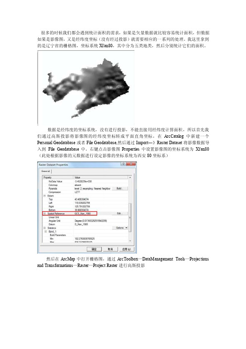
很多的时候我们都会遇到统计面积的需求,如果是矢量数据就比较容易统计面积,但数据如果是影像图,又是经纬度坐标(没有经过投影)就需要相应的一系列的处理。
我这里拿到的是辽宁省的栅格图,坐标系统Xi'an80,其中分为五类地类,然后分别统计它们的面积。
数据是经纬度的坐标系统,没有进行投影,不能直接用经纬度计算面积,所以首先我们通过高斯投影将影像图的经纬度坐标转成平面直角坐标,在ArcCatalog中新建一个Personal Geodatabase或者File Geodatabase,然后通过Import---》Raster Dataset将影像数据导入到File Geodatabase中。
右键点击影像图Properties中设置影像图的坐标系统为Xi'an80(此处根据影像的元数据进行设定影像的坐标系统为西安80坐标系)然后在ArcMap中打开栅格图,通过ArcToolbox—DataManagement Tools—Projections and Transformations—Raster—Project Raster进行高斯投影投影之后,就可以进行分类计算了,将投影后的影像图通过栅格分析工具进行重分类,选择Spatial Analyst工具栏下拉菜单的“Reclassify…”项在重分类后的影像上点击鼠标右键,选择“Open Attribute Table”其中COUNT字段中的数值时代表每类地物中所包含的像素个数,这样的话我们就可以通过像素个数*每个像素的面积=影像图的面积,如何获得每个像素所代表的面积,在重分类后的影像上点击鼠标右键,选择“properties…”,在弹出的layer properties窗口中择“Source”选项栏,CellSize项的值为单元格大小信息。
最后通过Field Calculator可以计算出面积,可以把计算出来的值存放到另外一个字段里文案编辑词条B 添加义项?文案,原指放书的桌子,后来指在桌子上写字的人。
关于矢量数据叠加分析的教程
项,在Pro-logic VBA Script Code文本框内输入以下VBA代码:(“//”右边的文
字为代码说明,不必输入,只输入英文代码即可)
dim newarea as double //声明double类变量newarea用于保存面积值,该名
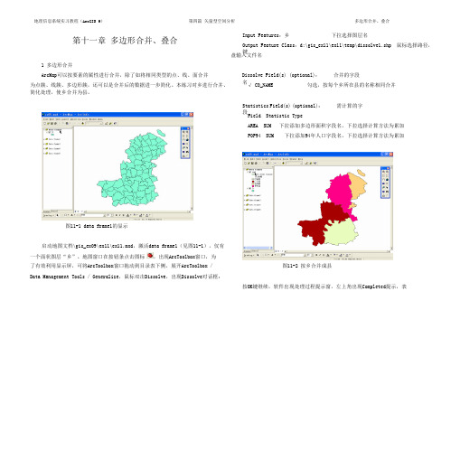
地理信息系统实习教程(ArcGIS 9) 第四篇 矢量型空间分析 多边形合并、叠合
11 - 2
示处理完毕,按Close键关闭。叠合后的图层dissolve1出现在目录表、地图窗口
内(见图11-2)。每个乡按所在县合并,空间处理的结果是取消了多边形乡的边
界,保留了县的边界,对AREA和POP94二个字段作了累加计算。
到这二个图层名出现在Features列表中。
Output Feature Class:d:\gis_ex09\ex11\temp\Union1.shp 鼠标选择路径,键
盘输入文件名
JoinAttributes (Optional):ALL 默认,所有字段都合并
按OK键继续,软件出现处理过程提示窗,左上角出现Completed提示,处
字可以自行取名,但要与下面的命令框输入的名字
保持一致
dim pArea as IArea //声明IArea类变量pArea用于保存参与计算的字段
set pArea = [shape] //为变量pArea赋值
newarea = pArea.area //求解多边形面积并赋给以上用户定义的变量
newarea
独立属性表found.dbf,用Add按钮,该表加载。鼠标右键点击该表,选Open打
HFSS的前、后处理

4-15
4-16
Ansoft HFSS的后处理(Radiation)
Radiation
4-17
HFSS Field Calculator: Definition
A tool for performing mathematical operations on ALL saved field data in the modeled geometry
Driven Modal Driven Terminal Eigenmode
Validation Checking
用于检验模型的可行性
4-3
设置解算类型:
设置解算类型:
本节将介绍如何设置解算类型。解算类型决定求解结果的类型, 确定如何激励和收敛。HFSS有以下几种解算类型: 模式驱动(Driven Modal):这种解算类型计算以模式为基础的 S参数。根据波导模式的入射和反射功率表示S参数矩阵的解。 终端驱动(Driven Terminal): 这种解算类型计算以终端为基础 的多导体传输线端口的S参数。此时,根据传输线终端的电压和 电流表示S参数矩阵的解。 本征模(Eignemode):计算某一结构的本征模式或谐振.本征模 解算器可以求出该结构的谐振频率以及这些谐振频率下的场模式 。 模式驱动(Driven Modal):模式S参数的差值▽S.这是以前版本 驱动解唯一可以提供的收敛方法. 终端驱动(Driven Terminal): 单端或不同节点S参数的差值 ▽S。 本征模(Eignemode): 频率差值▽F.
4-5
激励设置
HFSS的求解设置
网格设置
GIS缓冲区分析2
上机练习2目标:使用ArcToolbox掌握最基本的空间分析操作,即缓冲区分析(也称邻近区分析)。
缓冲区分析(Buffer)是对选中的一组或一类地图要素(点、线或面)按设定的距离条件,围绕其要素而形成一定缓冲区多边形实体,从而实现数据在二维空间得以扩展的信息分析方法。
缓冲区应用的实例有如:污染源对其周围的污染量随距离而减小,确定污染的区域;为失火建筑找到距其500米范围内所有的消防水管等。
ArcGIS提供多种方式执行同一功能,主要包括:(1)使用ArcToolbox中的工具();(2)使用ArcGIS内置的命令(Command);(3)使用专门的工具条(Toolbar)。
以下将分别练习前两种实现空间分析Buffer的方法。
数据:a.仓库(面状,warehouse.shp),用来产生多边形要素的邻近区b.道路(线状,road.shp),用于地图显示和道路密度的计算c.铁路(线状,railway.shp),用来产生线状要素的邻近区d.道路1(线状,road1.shp),仅用于地图显示,不参加分析e.区域界线(面状,bound.shp),用来计算道路密度f.公园(点状,park.shp),用来产生基于网络的服务区操作步骤:一、产生多边形要素的邻近区要求:对存储危险品的仓库,规定在存储基地周围100米范围内不准有建筑物,也不准存放易燃易爆物品;周围200米范围内可以有一般建筑物,但不能有易燃易爆物品;周围300米范围内不准建设住宅,以及商业、学校、办公等设施。
为实现上述要求,须对仓库要素产生100、200、300米的邻近区。
1.打开ArcMap应用程序,创建空地图,使用标准工具条中的按钮添加存放在文件夹F:\Spatial Analysis\Exercises\ex02中的warehouse和road数据层。
2.为地图设置距离单位和显示单位。
有两种方式进入设置单位的对话框,一种是选中数据组(在目录中显示为Layers),双击打开“Data Frame Properties”对话框;另一种方法是在选中数据组后,单击鼠标右键,弹出快捷菜单,选择最后一栏Properties。
ansoft后处理过程中计算器使用方法英文版
ANSOFT MAXWELL 2D/3D FIELD CALCULATOR-Examples-IntroductionThis manual is intended as an addendum to the on-line documentation regarding Post-processing in general and the Field Calculator in particular. The Field Calculator can be used for a variety of tasks, however its primary use is to extend the post-processingcapabilities within Maxwell beyond the calculation / plotting of the main field quantities.The Field Calculator makes it possible to operate with primary vector fields (such as H, B, J, etc) using vector algebra and calculus operations in a way that is both mathematically correct and meaningful from a Maxwell’s equations perspective.The Field Calculator can also operate with geometry quantities for three basic purposes:-plot field quantities (or derived quantities) onto geometric entities;-perform integration (line, surface, volume) of quantities over specified geometric entities;-export field results in a user specified box or at a user specified set of locations (points).Another important feature of the (field) calculator is that it can be fully macro driven. All operations that can be performed in the calculator have a corresponding “image” in one or more lines of macro language code. Post-processing macros are widely used forrepetitive post-processing operations, for support purposes and in cases whereOptimetrics is used and post-processing macros provide some quantity required in the optimization / parameterization process.This document describes the mechanics of the tools as well as the “softer” side of it as well. So, apart from describing the structure of the interface this document will show examples of how to use the calculator to perform many of the post-processing operations encountered in practical, day to day engineering activity using Maxwell. Examples are grouped according to the type of solution. Keep in mind that most of the examples can be easily transposed into similar operations performed with solutions of different physical nature. Also most of the described examples have easy to find 2D versions.1.Description of the interfaceThe interface is shown in Fig. I1. It is structured such that it contains a stack which holds the quantity of interest in stack registers. A number of operations are intended to allow the user to manipulate the contents of the stack or change the order of quantities being hold in stack registers. The description of the functionality of the stack manipulationbuttons (and of the corresponding stack commands) is presented below:-Push repeats the contents of the top stack register so that after the operation the two top lines contain identical information;-Pop deletes the last entry from the stack (deletes the top of the stack);-RlDn(roll down) is a “circular” move that makes the contents of the stacks slide down one line with the bottom of the stack advancing to the top;-RlUp (roll up) is a “circular” move that makes the contents of the stacks slide up one line with the top of the stack dropping to the bottom;-Exch (exchange) produces an exchange between the contents of the two top stack registers;-Clear clears the entire contents of all stack registers;-Undo reverses the result of the most recent operation.Fig. I1 Field Calculator Interface Stack & stack registersStackcommandsCalculatorbuttonsThe user should note that Undo operations could be nested up to the level where a basic quantity is obtained.The calculator buttons are organized in five categories as follows:-Input contains calculator buttons that allow the user to enter data in the stack; sub-categories contain solution vector fields (B, H, J, etc.), geometry(point, line surface,volume), scalar, vector or complex constants (depending on application) or even entiref.e.m. solutions.-General contains general calculator operations that can be performed with “general”data (scalar, vector or complex), if the operation makes sense; for example if the top two entries on the stack are two vectors, one can perform the addition (+) but notmultiplication (*);indeed, with vectors one can perform a dot product or a cross product but not a multiplication as it is possible with scalars.-Scalar contains operations that can be performed on scalars; example of scalars are scalar constants, scalar fields, mathematical operations performed on vector which result in a scalar, components of vector fields (such as the X component of a vector field), etc.-Vector contains operations that can be performed on vectors only; example of such operations are cross product (of two vectors), div, curl, etc.-Output contains operations resulting in plots (2D / 3D), graphs, data export, data evaluation, etc.As a rule, calculator operations are allowed if they make sense from a mathematical point of view. There are situations however where the contents of the top stack registers should be in a certain order for the operation to produce the expected result. The examples that follow will indicate the steps to be followed in order to obtain the desired result in anumber of frequently encountered operations. The examples are grouped according to the type of solution (solver) used. They are typical medium/higher level post-processing task that can be encountered in current engineering practice. Throughout this manual it is assumed that the user has the basic skills of using the Field Calculator for basicoperations as explained in the on-line technical documentation and/or during Ansoft basic training.Note: The f.e.m. solution is always performed in the global (fixed) coordinate system.The plots of vector quantities are therefore related to the global coordinate system and will not change if a local coordinate system is defined with a different orientation from the global coordinate system.The same rule applies with the location of user defined geometry entities for post-processing purposes. For example the field value at a user-specified location (point)doesn’t change if the (local) coordinate system is moved around. The reason for this isthat the coordinates of the point are represented in the global coordinate systemregardless of the current location of the local coordinate system.Electrostatic ExamplesExample ES1: Calculate the charge density distribution and total electric charge on the surface of an objectDescription: Assume an electrostatic (3D) application with separate metallic objects having applied voltages or floating voltages. The task is to calculate the total electric charge on any of the objects.a)Calculate/plot the charge density distribution on the object; the sequence of calculatoroperations is described below:-Qty -> D (load D vector into the calculator);-Geom -> Surface… (select the surface of interest)-> OK-Unit Vec -> Normal (creates the normal unit vector corresponding to the surface of interest)-Dot (creates the dot product between D and the unit normal vector to the surface of interest, equal to the surface charge density)-Geom -> Surface… (select the surface of interest)-> OK-Plotb)Calculate the total electric charge on the surface of an object-Qty -> D (load D vector into the calculator);-Geom -> Surface… (select the surface of interest)-> OK-Normal--EvalExample ES2: Calculate the Maxwell stress distribution on the surface of an objectDescription: Assume an electrostatic application (for ex. a parallel plate capacitorstructure). The surface of interest and adjacent region should have a fine finite element mesh since the Maxwell stress method for calculation the force is quite sensitive to mesh.The Maxwell electric stress vector has the following expression for objects withoutelectrostrictive effects:()221E n E n D T nEερρρρ-⋅=where the unit vector n is the normal vector to the surface of interest. The sequence of calculator commands necessary to implement the above formula is given below.- Qty -> D- Geom -> Surface… (select the surface of interest) -> OK- Unit Vec -> Normal (creates the normal unit vector corresponding to the surface of interest) - Dot - Qty -> E - * (multiply)- Geom -> Surface… (select the surface of interest) -> OK- Unit Vec -> Normal (creates the normal unit vector corresponding to the surface of interest) - Num ->Scalar (0.5) OK - * - Const -> Epsi0 - * - Qty -> E - Push - Dot - * - - (minus)- Geom -> Surface… (select the surface of interest) -> OK -PlotIf an integration of the Maxwell stress is to be performed over the surface of interest, then the Plot command above should be replaced with the following sequence:- Normal - ⎰-EvalNote: The surface in all the above calculator commands should lie in free space or should coincide with the surface of an object surrounded by free space (vacuum, air). It should also be noted that the above calculations hold true in general for any instance where a volume distribution of force density is equivalent to a surface distribution of stress (tension): dS T dv f F v n ⎰⎰∑∑==ρρρwhere Tn is the local tension force acting along the normal direction to the surface and F is the total force acting on object(s) inside ∑.The above results for the electrostatic case hold for magnetostatic applications if the electric field quantities are replaced with corresponding magnetic quantities.Current flow ExamplesExample CF1: Calculate the resistance of a conduction path between two terminalsDescription: Assume a given conductor geometry that extends between two terminals with applied DC currents.In DC applications (static current flow) one frequent question is related to the calculation of the resistance when one has the field solution to the conduction (current flow) problem. The formula for the analytical calculation of the DC resistance is:()()⎰⋅=CDC s A s dsR σwhere the integral is calculated along curve C (between the terminals) coinciding with the “axis” of the conductor. Note that both conductivity and cross section area are in general function of point (location along C). The above formula is not easily implementable in the general case in the field calculator so that alternative methods to calculate the resistance must be found.One possible way is to calculate the resistance using the power loss in the respective conductor due to a known conduction current passing through the conductor. 2DC DC I P R = where power loss is given by dV J J dV J E P V Vρρρρ⋅=⋅=⎰⎰σThe sequence of calculator commands to compute the power loss P is given below:-Qty -> J - Push- Num -> Scalar (1e7) OK (conductivity assumed to be 1e7 S/m) - / (divide) - Dot- Geom -> Volume… (select the volume of interest) -> OK - ⎰-EvalThe resistance can now be easily calculated from power and the square of the current.There is another way to calculate the resistance which makes use of the well known Ohm’s law.IU R DCAssuming that the conductor is bounded by two terminals, T1 and T2 (current through T1 and T2 must be the same), the resistance of the conductor (between T1 and T2) is given the ratio of the voltage differential U between T1 and T2 and the respective current, I . So it is necessary to define two points on the respective terminals and then calculate the voltage at the two locations (voltage is called Phi in the field calculator). The rest is simple as described above.Example CF2: Export the field solution to a uniform gridDescription: Assume a conduction problem solved. It is desired to export the field solution at locations belonging to a uniform grid to an ASCII file.The field calculator allows the field solutions to be exported regardless of the nature of the solution or the type of solver used to obtain the solution. It is possible to export any quantity that can be evaluated in the field calculator. Depending on the nature of the data being exported (scalar, vector, complex), the structure of each line in the output file is going to be different. However, regardless of what data is being exported, each line in the data section of the output file contains the coordinates of the point (x, y, z) followed by the data being exported (1 value for a scalar quantity, 2 values for a complex quantity, 3 values for a vector in 3D, 6 values for a complex vector in 3D)To export the current density vector to a grid the field calculator steps are: - Qty J- Export -> On Grid (then fill in the data as appropriate, see Fig. CF2) - OKFig. CF2 Define the size of the export region (box) and spacing withinMinimum, maximum & spacing in all 3 directions X, Y, Z define the size of therectangular export region (box) as well as the spacing between locations. By default the location of the ASCII file containing the export data is in the project directory. Clicking on the browse symbol one can also choose another location for the exported file.Note: One can export the quantity calculated with the field calculator at user specified locations by using the Export/To File command. In that case the ASCII file containing on each line the x, y and z coordinates of the locations must exist prior to initiating theexport-to-file command.Example CF3: Calculate the conduction current in a branch of a complex conduction pathDescription:There are situations where the current splits along the conduction path. If the nature of the problem is such that symmetry considerations cannot be applied, it may be necessary to evaluate total current in 2 or more parallel branches after the split point.To be able to perform the calculation described above, it is necessary to have eachparallel branch (where the current is to be calculated) modeled as a separate solid.Before the calculation process is started, make sure that the (local) coordinate system is placed somewhere along the branch where the current is calculated, preferably in amedian location along that branch. In more general terms, that location is where theintegration is performed and it is advisable to choose it far from areas where the current splits or changes direction, if possible.Here is the process to be followed to perform the calculation using the field calculator.-Qty -> J- Geom -> Volume… (choose the volume of the branch of interest) OK- Domain (this is to limit the subsequent calculations to the branch of interest only)-Geom -> Surface… yz (choose axis plane that cuts perpendicular to the branch) OK - Normal - ⎰- EvalThe result of the evaluation is positive or negative depending on the general orientation of the J vector versus the normal of the integration surface (S). In mathematical terms the operation performed above can be expressed as:⎰⋅=SdS n J I ρρNote: The integration surface (yz, in the example above) extends through the whole region, however because of the “domain” c ommand used previously, the calculation is restricted only to the specified solid (that is the S surface is the intersection between the specified solid and the integration plane).Magnetostatic examplesExample MS1: Calculate (check) the current in a conductor using Ampere’s theoremDescription: Assume a magnetostatic problem where the magnetic field is produced by a given distribution of currents in conductors. To calculate the current in the conductor using Ampere’s theorem, a closed polyline (of arbitrary shape) shou ld be drawn around the respective conductor. In a mathematical form the Ampere’s theorem is given by:⎰ΓΓ⋅=s d H I S ρρwhere Γ is the closed contour (polyline) and S Γ is an open surface bounded by Γ but otherwise of arbitrary shape. I S Γ is the total current intercepting the surface S Γ.To calculate the (closed) line integral of H, the sequence of field calculator commands is:- Qty -> H - Geom -> Line (choose the closed polygonal line around the conductor) OK - Tangent - ⎰-EvalThe value should be reasonably close to the value of the corresponding current. Thematch between the two can be used as a measure of the global accuracy of the calculation in the general region where the closed line was placed.Example MS2: Calculate the magnetic flux through a surfaceDescription: Assume the case of a magnetostatic application. To calculate the magnetic flux through an already existing surface the sequence of calculator commands is: -Qty -> B -Geom -> Surface… (specify the integration surface) OK -Normal -⎰ - EvalThe result is positive or negative depending on the orientation of the B vector with respect to the normal to the surface of integration.The above operation corresponds to the following mathematical formula for the magnetic flux:⎰⋅=ΦSS dA n B ρρExample MS3: Calculate components of the Lorentz forceDescription: Assume a distribution of magnetic field surrounding conductors with applied DC currents. The calculation of the components of the Lorentz force has the following steps in the field calculator. -Qty -> J <curl H> -Qty -> B -Cross -Scalar -> ScalarX -Geom -> Volume … (specify the volume of interest) OK -⎰ - EvalThe above example shows the process for calculating the X component of the Lorentz force. Similar steps should be performed for all components of interest.Example MS4: Calculate the distribution of relative permeability innonlinear materialDescription: Assume a non-linear magnetostatic problem. To plot the relativepermeability distribution inside a non-linear material the following steps should be taken: -Qty -> B-Scal? -> ScalarX-Qty -> H-Scal? -> ScalarX-Const -> Mu0-* (multiply)-/ (divide)-Smooth-Geom -> Surface… (specify the geometry of interest)OK-PlotAs an example of distribution of relative permeability please take a look at plot in Fig.MS 4.Fig. MS4 Distribution of relative permeability (saturation)Note: The above sequence of commands makes use of one single field component (X component). Please note that any spatial component can be used for the purpose ofcalculating relative permeability in non-linear soft magnetic materials. The result would still be the same if we used the Y component or the Z component. The “smoothing” also used in the sequence is also recommended particularly in cases where the mesh density is not very high.Frequency domain (AC) ExamplesExample AC1: Calculate the radiation resistance of a circular loopDescription: Assume a circular loop of radius 0.02 m with an applied current excitation at 1.5 GHz; The radiation resistance is given by the following formula: 2rms av r I P R = ()()dS H H j dS H E P S S av ⎰⎰⎰⎰⎥⎦⎤⎢⎣⎡⨯⨯∇=⨯=*0*1Re 21Re 21ρρρρωε where S is the outer surface of the region (preferably spherical), placed conveniently far away from the source of radiation. Assuming that a half symmetry model is used, no ½ is needed in the above formula. The sequence of calculator commands necessary for the calculation of the average power is as follows: - Qty -> H -Curl -Num -> Complex (0 , -12) OK -* -Qty -> H -Cmplx -> Conj -Cross -Cmplx -> Real -Geom -> Surface…(select the surface of interest) -> OK -Normal -⎰ - EvalNote : The integration surface above must be an open surface (radiation surface) if a symmetry model is used. Surfaces of existing objects cannot be used since they are always closed. Therefore the necessary integration surface must be created in the example above using Geometry/Create/Faces List command.Example AC2: Calculate/Plot the Poynting vectorDescription: Same as in Example AC1.To obtain the Poynting vector the following sequence of calculator commands isnecessary:- Qty -> H-Curl-Num -> Complex (0 , -12) OK-*-Qty -> H-Cmplx -> Conj-CrossTo plot the real part of the Poynting vector the following commands should be added to the above sequence:…..-Cmplx -> Real-Num -> Scalar (0.5) OK-Geom -> Surface…(select the surface of interest)-> OK-PlotA plot similar to the one in Fig. AC2 is obtained.Fig. AC2 Distribution of the real part of the Poynting vectorExample AC3: Calculate total induced current in a solidDescription: Consider (as example) the device in Fig. AC3.a) full modelb) quarter modelFig. AC3 Geometry of inductor modelAssume that the induced current through the surface marked with an arrow in the quarter model is to be calculated. Please note that there is an expected net current flow through the market surface, due to the symmetry of the problem. As a general recommendation, the surface that is going to be used in the process of integrating the current density should exist prior to initiating the respective post-processing. In some cases this also means that the geometry needs to be created in such a way so that the particular post-processing task is made possible. Once the object containing the integration surface exists, after thesolution was calculated, while in the post-processor use the Geometry/Create/Faces List command to create the integration surface necessary for the calculation. Make sure that the object with expected induced currents has non-zero conductivity and that the eddy-effect calculation was turned on.Assuming now that all of the above was taken care of, the sequence of calculatorcommands necessary to obtain separately the real part and the imaginary part of theinduced current is described below:For the real part of the induced current:-Qty -> J-Cmplx -> Real-Geom -> Surface… (select the previously defined integration surface)OK-Normal--EvalFor the imaginary part of the induced current:-Qty -> J-Cmplx -> Imag-Geom -> Surface… (select the previously defined integration surface)OK-Normal-⎰-EvalIf instead of getting the real and imaginary part of the current , one desires to do an “a t phase” calculation, the sequence of commands is:-Qty -> J-Num -> Scalar (45) OK(assuming a calculation at 45 degrees phase angle)-Cmplx -> AtPhase-Geom -> Surface… (select the previously defined integration surface)OK-Normal-⎰-EvalExample AC4: Calculate (ohmic) voltage drop along a conductive pathDescription: Assume the existence of a conductive path (a previously defined open line totally contained inside a conductor). To calculate the real and imaginary components of the ohmic voltage drop inside the conductor the following steps should be followed:For the real part of the voltage:-Qty -> J-Matl -> Conductivity -> Divide OK-Cmplx -> Real-Geom -> Line (select the applicable line)OK-Tangent-⎰-EvalFor the imaginary part of the voltage:-Qty -> J-Matl -> Conductivity -> Divide OK-Cmplx -> Imag-Geom -> Line (select the applicable line)OK-Tangent-⎰-EvalTo calculate the phase of the voltage manipulate the contents of the stack so that the top register contains the real part of the voltage and the second register of the stack contains the imaginary part. To calculate phase enter the following command:- Trig -> Atan2Example AC5: Calculate the AC resistance of a conductorDescription:Consider the existence of an AC application containing conductors with significant skin effect. Assume also that the mesh density is appropriate for the task, i.e.mesh has a layered structure with 1-2 layers per skin depth for 3-4 skin depths if the conductor allows it. Here is the sequence to follow in order to calculate the total power dissipated in the conductor of interest.-Qty -> Ohmic-Loss-Geom -> Volume -> (specify volume of interest)OK--EvalNote: To obtain the AC resistance the power obtained above must be divided by the squared rms value of the current applied to the conductor. Note that in theBoundary/Source Manager peak values are entered for sources, not rms values.Time Domain ExamplesExample TD1: Creation of a post processing macroDescription: Assume a time domain (transient application) requiring the display of induced current as a function of time.Enter Cntrl-F1 and enter a macro name to start recording the macro.Enter Geometry/Create/FacesList, select the object and then the face(s) necessary for the calculation. Repeat the operation for all integration operation desired to be performed by the macro. Then select Data/Calculator to start the field calculator.The sequence of calculator commands is presented below. Please note that the geometry necessary for the macro (certain faces of objects) is also included in the macro.-Qty -> J<curl H>-Geom -> Surface… (enter the surface of interest)OK-Normal--Eval-Append (enter the name of the variable)Close the calculator and enter Cntrl-F2 to stop recording and to save the macro.# Version 1DefineFacesList "faces1"AddFaceWithId "faces1" "box3" 134……………………ShowCalcEnter "CurlH"EnterSurface "faces1"NormalComponentIntegrateEvaluateRenameEntry "curr_core"AppendSolutions "d:/maxwell/tr2_tr.pjt/tmpfiles/curr_core.tmp"The name (& path) of the macro must be specified in the Solution Setup window.Example TD2: Find the maximum/minimum field value/locationDescription: Consider a solved transient application. To find extreme field values in a given volume and/or the respective locations follow these steps.To get the value of the maximum magnetic flux density in a given volume:-Qty -> B-Mag-Geom -> Volume… (enter volume of interest)OK-Max -> Value-EvalTo get the location of the maximum:-Qty -> B-Mag-Geom -> Volume… (enter volume of interest)OK-Max -> Position-EvalThe process is very similar when searching for the minimum. Just replace the Max with Min in the above sequences.Example TD3: Find the iso-surface of a given value inside a given object Description: Assume a solved application. Find the surface (inside an object) where the magnetic flux density magnitude has a user-specified value.The sequence of commands is as follows.-Qty -> B-Mag-Geom -> Volume … (enter volume of interest) OK-Domain-Num -> Scalar… (0.3)OK (0.3 is the value on the iso-surface)-Iso-DrawThe result of the operation is a surface. The result can be used in subsequent operations involving a surface. For example it can be used for integration purposes.Note: The iso-value entered above must be realistic. If an iso-surface with the specified value cannot be found, an error message is displayed.Example TD4: Combine (by summation) the solutions from two time steps Description: Assume a linear model transient application. It is possible to add thesolution from different time steps if you follow these steps:First enter the post-processor to post-process the solution at a certain time step, say t1.Then in the calculator:-Qty -> B-Write (enter the name of the file)OKExit the post-processor and re-enter at a different time step, say t2.Then, in the calculator:-Qty -> B-Read (specify the name of the .reg file to be read in)OK-+ (add)-Mag-Geom -> Surface… (enter surface of interest)OK。
dwg文件点提取高程
dwg文件点提取高程(最新版)目录1.DWG 文件简介2.点提取高程的方法3.高程数据的应用4.总结正文一、DWG 文件简介DWG(Drawing)文件是一种常用于工程设计和建筑领域的矢量图形文件格式。
它由 AutoCAD 开发,并用于存储二维和三维图形信息。
DWG 文件中包含了各种设计元素,如线条、多边形、文本和点等。
在众多应用场景中,点是表示地形高程的一种常见方式。
二、点提取高程的方法提取 DWG 文件中的高程点,通常采用以下几种方法:1.使用 AutoCAD 软件:作为 DWG 文件的创建者,AutoCAD 提供了一系列的工具和命令来提取高程点。
用户可以利用 AutoCAD 的“点”命令创建高程点,然后使用“高程”命令或“属性”命令查询高程值。
2.使用 GIS 软件:许多 GIS 软件,如 ArcGIS、QGIS 等,都可以读取 DWG 文件。
用户可以将 DWG 文件导入到 GIS 软件中,然后利用GIS 工具提取高程点。
例如,在 ArcGIS 中,可以使用“Make XY Event Layer”工具将 DWG 文件转换为点要素层,再使用“Field Calculator”工具计算高程值。
3.使用编程语言:如果需要自动化处理大量 DWG 文件,可以使用编程语言(如 Python)结合相应库(如 PyAutoCAD、Geopandas 等)来实现点提取高程的功能。
三、高程数据的应用提取出的高程点可以用于多种应用场景,如地形分析、工程测量、城市规划等。
高程数据的处理和分析,可以借助 GIS 软件或编程语言来完成。
例如,可以利用 GIS 软件进行地形分析,计算坡度、坡向等地形指标;也可以利用编程语言进行高程数据的可视化,生成三维地形图等。
四、总结通过以上方法,我们可以从 DWG 文件中提取高程点,并将其应用于各种实际场景。
需要注意的是,根据实际需求和数据量,选择合适的方法和工具来完成任务。
arcgis 提取字段
arcgis 提取字段【最新版】目录1.ArcGIS 简介2.提取字段的目的和方法3.常用提取字段工具4.提取字段的步骤5.提取字段的应用案例正文一、ArcGIS 简介ArcGIS 是一款由美国环境系统研究所(Esri)公司开发的地理信息系统(GIS)软件。
它广泛应用于地理信息数据的采集、管理、分析和可视化等领域,为各个行业提供了强大的空间数据处理能力。
在 ArcGIS 中,用户可以利用各种工具和函数完成地理信息的处理和分析任务。
二、提取字段的目的和方法在 ArcGIS 中,提取字段是指从地理信息数据中选取特定的字段,以便进行进一步的分析和处理。
提取字段的目的主要包括:减少数据量、优化数据结构、方便数据查询和分析等。
提取字段的方法主要有以下几种:1.使用“提取字段”工具:ArcGIS 工具箱中的“提取字段”工具(如“Make Fields”),可以方便地对地理信息数据进行字段提取。
2.使用“字段计算器”:在 ArcGIS 中,用户可以使用“字段计算器”根据已有字段计算出新的字段。
3.使用 Python 脚本:通过编写 Python 脚本,用户可以实现更复杂的字段提取需求。
三、常用提取字段工具在 ArcGIS 中,有以下几种常用的提取字段工具:1.“Make Fields”工具:位于“ArcToolbox”工具箱中的“Spatial Analyst Tools”组,可用于提取点、线、面等地理信息数据的字段。
2.“Field Calculator”工具:位于“ArcToolbox”工具箱中的“Spatial Analyst Tools”组,可用于对地理信息数据的字段进行计算和转换。
3.“Python Parser”工具:位于“ArcToolbox”工具箱中的“Conversion Tools”组,可用于将 Python 脚本中的字段提取操作应用到地理信息数据上。
四、提取字段的步骤以“Make Fields”工具为例,提取字段的步骤如下:1.打开 ArcGIS 软件,加载需要提取字段的地理信息数据。
- 1、下载文档前请自行甄别文档内容的完整性,平台不提供额外的编辑、内容补充、找答案等附加服务。
- 2、"仅部分预览"的文档,不可在线预览部分如存在完整性等问题,可反馈申请退款(可完整预览的文档不适用该条件!)。
- 3、如文档侵犯您的权益,请联系客服反馈,我们会尽快为您处理(人工客服工作时间:9:00-18:30)。
Field Calculator 的使用
Field Calculator 工具可以在属性表字段点击右键,选择“Field Calculator ”,或者Data Management
Tools->fields-> Calculate Field打开。
1.基本函数
针对数值型:
Abs:求绝对值
Atn:求反正切值
Cos:求余弦值
Exp:求反对数值
Fix:取整数部分,与 Int 函数有区别的
Int:取整数部分
Int 和 Fix 函数的区别在于如果 number 参数为负数时,Int 函数返回小于或等于 number 的第一个负
整数,而 Fix 函数返回大于或等于 number 参数的第一个负整数。
MyNumber = Int(99.8) ' 返回 99。
MyNumber = Fix(99.2) ' 返回 99。
MyNumber = Int(‐99.8) ' 返回‐100。
MyNumber = Fix(‐99.8) ' 返回‐99。
MyNumber = Int(‐99.2) ' 返回‐100。
MyNumber = Fix(‐99.2) ' 返回‐99。
Log:求对数值
Sin:求正弦值
Sqr:开方
Tan:求正切
针对字符串型:
Asc:返回与字符串的第一个字母对应的 ANSI 字符代码
Chr:将一个 ASCII 码转为相应的字符,与它对应的是 ASC()函数
Format:返回根据格式 String 表达式中包含的指令设置格式的字符串,例如Format(13.3,"0.00")=13.30
Instr:返回某字符串在另一字符串中第一次出现的位置
LCase:返回字符串的小写格式,例如 LCase("ARCGIS")="arcgis"
Left:返回字符串左边的内容,例如 Left("arcgis",2)="ar" ,把[A]字段的前2个字符赋给[B]
Len:返回字符串的长度,例如 Len("arcgis")=6
LTrim:去掉字符串左边的空格,例如 LTrim(" arcgis")="arcgis"
Mid:取出字符串中间的内容,例如 Mid("arcgis",2,1)="r" 在name字段前四个字符后面加一个空格,left([name],4) & " " & mid([name],5)
QBColor:返回一个 Integer 值,该值表示对应于指定的颜色编号的 RGB 颜色代码
Right:返回字符串右边的内容,例如 Right("arcgis",2)="is"
RTrim:去掉字符串右边的空格,例如 RTim("arcgis ")="arcgis"
Space:返回由指定数量空格组成的字符串,例如 MyString = "Hello" & Space(10) & "World" ' 在两个字符串
之间插入 10 个空格。
StrConv:返回按照指定方式转换的字符串。
String:将对象转换为字符串。
Trim:去掉字符串前后的空格,例如 Trim(" arcgis ")="arcgis"
UCase:返回字符串的大写格式,例如 UCase("arcgis")="ARCGIS"
针对日期类型:
Date:获取日期
DateAdd:返回一个 Date 值,其中包含已添加指定时间间隔的日期和时间值。
DateDiff:两个日期之间存在的指定时间间隔的数目
DatePart:用于计算日期并返回指定的时间间隔
Now:获取日期+时间
2.简单VBA
把属性值1、2、3换成A、B、C
Dim sResult as string
Dim sField as string
sField = [字段名]
If (sField="1") Then
sResult ="A"
ElseIf (sField="2") Then
sResult ="B"
ElseIf (sField="3") Then
sResult ="C"
End If。