The Rich Are Different! Pareto Law from asymmetric interactions in asset exchange models
泰尔指数资料

泰尔指数泰尔指数是一种衡量收入或财富分配不平等程度的指标,最初由意大利经济学家冯·泰尔于1912年提出。
它常被用来评估一个国家、地区或群体内个体之间收入或财富分配的不均衡程度。
泰尔指数的计算方法泰尔指数的计算方法相对简单,通常基于收入或财富在总体中相对的份额来确定。
假设有n个单位(个人、家庭或其他单位),第i个单位的收入或财富比例为pi(i=1,2,…,n),总的收入或财富比例为P。
泰尔指数的计算公式为:\[T = \frac{1}{2} \sum_{i=1}^{n} \sum_{j=1}^{n} \frac{1}{n^2} |p_i - p_j|\]其中,|pi - pj|表示第i个和第j个单位之间的差距;n为单位的总数。
泰尔指数的取值范围为[0,1],值越接近0则表示收入或财富分配越趋于平等,反之越接近1则表示分配越不平等。
泰尔指数的应用泰尔指数广泛应用于经济学、社会学等领域,可以帮助研究人员量化不平等情况并进行比较。
在政策制定和社会政治决策中,泰尔指数也扮演着重要的角色。
政府和国际组织通常会根据泰尔指数等指标来评估经济状况、贫富差距,进而采取相应的政策来促进社会公平和稳定。
泰尔指数的局限性虽然泰尔指数是一种常用的衡量不平等程度的指标,但也存在一些局限性。
首先,泰尔指数只能提供总体不平等的概览,无法深入到个体或具体群体的情况。
其次,泰尔指数对极端值或异常值比较敏感,可能受到极端富有或贫穷个体的影响。
此外,泰尔指数本质上是一种相对指标,不同国家、地区或文化背景下的比较需要谨慎对待。
结语泰尔指数作为一种常用的不平等度量工具,为我们提供了一个客观评估不平等现象的视角。
虽然存在一些局限性,但在适当的情况下,泰尔指数仍然可以为我们提供有价值的信息,帮助我们更好地了解和应对不平等问题。
希望通过对泰尔指数的了解,可以引起更多人对不平等问题的关注,促进社会的公平和持续发展。
范里安-微观经济学现代观点-第8版-第八版-ch13-风险资产(含全部习题解答)-东南大学曹乾
Intermediate Microeconomics:A Modern Approach (8th Edition)Hal R. Varian范里安中级微观经济学:现代方法(第8版)完美中文翻译版)含全部习题详细解答)第13章:风险资产(含全部习题详细解答风险资产(曹乾译(东南大学caoqianseu@)13风险资产在上一章,我们分析了不确定性情形下的个人行为模型,以及保险市场和股票市场这两种经济制度的作用。
在本章我们进一步分析股票市场如何分散风险的。
为做此事,最好从一个简化的不确定性行为模型进行分析。
13.1均值—方差效用在上一章我们分析了不确定性情形下的选择问题,我们是用期望效用函数进行分析的。
这样的问题还有另外一类分析方法,即用一些参数(parameters )描述选择的目标,然后将效用函数视为这些参数的函数。
这类方法中最为流行的就是均值..—.方差模型....(mean-variance model )。
在均值—方差方法中,我们不再认为消费者的偏好取决于他的财富在每种可能结果上的整个概率分布,而是假设他的偏好可用几个关于他财富概率分布的统计量进行描述。
令随机变量w 取值s w 的概率为s π(其中S s ,...,2,1=)。
w 概率分布的均值..(mean )就是它的加权平均值:s Ss s w w ∑==1πµ.上式就是加权平均值的计算公式:每个结果s w 以它自身发生的概率s π作为权重(即s s w π),然后全部相加(一)。
w 概率分布的方差..(variance )是2)(w u w −的加权平均值: 212)(w S s s wu w −=∑=πσ. 方差衡量分布的“分散性”,因此可用来衡量风险。
还有一种相近的衡量方法,称为标准差...(standard deviation ),用w σ表示,它是方差的平方根:2w w σσ=.概率分布的均值衡量它的加权平均值,即这些分布围绕着的那个数值。
浪波比尔定律

浪波比尔定律浪波比尔定律是什么?浪波比尔定律(Bill's Law of Waves)是指在任何一个群体中,20%的人会掌握80%的资源和权力。
这个定律最初由意大利经济学家维尔弗雷多·帕累托(Vilfredo Pareto)提出,后来被美国社会学家约瑟夫·马修斯(Joseph M. Juran)和W. Edwards Deming等人进一步发展和应用。
为什么会有浪波比尔定律?浪波比尔定律的原因在于,在任何一个群体中,人们的能力、贡献和机遇都是不平等的。
有些人天生就具备了更多的天赋和才华,有些人则具备更好的机遇和资源,这使得他们在竞争中更容易脱颖而出。
同时,在一个群体中,有些人也更善于利用自己所拥有的资源去获取更多的资源,这也加剧了不平等现象。
如何应对浪波比尔定律?1. 了解自己所处环境要想应对浪波比尔定律,首先需要了解自己所处环境。
只有深入了解自己所在行业、公司或社交圈子中的资源和权力分布情况,才能更好地制定应对策略。
2. 建立良好的人际关系建立良好的人际关系是应对浪波比尔定律的重要手段之一。
通过与他人建立良好的关系,可以获取更多的资源和机会,同时也可以获得更多的支持和帮助。
3. 提高自己的能力提高自己的能力是应对浪波比尔定律最根本的方法。
只有不断提升自己的技能和知识水平,才能在竞争中更具优势,获得更多的机会和资源。
4. 创新和创造价值创新和创造价值也是应对浪波比尔定律的有效手段之一。
通过创新和创造价值,可以打破原有资源分配方式,开辟新的机会和领域。
5. 寻找合适的机会寻找合适的机会也是应对浪波比尔定律重要的策略之一。
只有找到适合自己发挥优势、获取资源和机会的领域,才能更好地应对浪波比尔定律带来的挑战。
浪波比尔定律的应用领域浪波比尔定律在经济学、管理学、市场营销等领域都有广泛的应用。
在经济学中,它被用来解释财富和收入的分配不均现象;在管理学中,它被用来解释组织中权力和资源的分配不均现象;在市场营销中,它被用来解释顾客行为和消费习惯的分布规律。
斯威齐模型概念

斯威齐模型概念解析1. 概念定义斯威齐模型(Pareto distribution),又称为洛伦兹曲线(Lorenz curve),是一种描述不平等分布的概率分布模型。
该模型是由意大利经济学家维尔弗雷多·斯威齐(Vilfredo Pareto)于1896年提出的,用于描述经济和社会领域中收入、财富、权力等指标的分布情况。
斯威齐模型的数学表达为:f(x)=k x k+1其中,x是一个正数,k是一个正参数,f(x)是x的概率密度函数。
2. 关键概念2.1 洛伦兹曲线洛伦兹曲线是斯威齐模型的可视化表示方法,用于展示不平等分布情况。
在洛伦兹曲线上,横坐标表示累积人口或累积收入比例(从小到大排列),纵坐标表示相应累积总收入比例。
通过绘制洛伦兹曲线可以直观地看出不同群体之间收入或财富的分布情况。
2.2 基尼系数基尼系数是衡量不平等程度的指标,通常与洛伦兹曲线一起使用。
基尼系数的取值范围为0到1,数值越大表示不平等程度越高。
基尼系数通过计算洛伦兹曲线下方面积与对角线下方面积的比值得到,公式如下:G=A A+B其中,A表示洛伦兹曲线下方面积,B表示对角线下方面积。
2.3 斯威齐指数斯威齐指数是斯威齐模型中的一个重要参数,用于描述分布的形状。
斯威齐指数越大,说明不平等程度越高。
斯威齐指数可以通过对斯威齐模型进行参数估计得到。
2.4 少部分财富或收入集中现象斯威齐模型描述了财富或收入在社会中的不平等分布情况。
根据该模型,少部分人拥有了大部分的财富或收入,而大多数人只能分享剩余的少部分。
这种现象被称为少部分财富或收入集中现象,也是斯威齐模型的核心概念之一。
3. 重要性3.1 揭示社会不平等问题斯威齐模型能够客观地描述经济和社会领域中财富、收入、权力等指标的分布情况。
通过洛伦兹曲线和基尼系数,可以直观地展示出不同群体之间的不平等程度,揭示出社会中存在的不公平现象。
3.2 政策制定依据斯威齐模型为政策制定提供了重要依据。
异质性时间偏好与资产定价

本文的模型丰富了异质性资产定价理论这一方 兴未艾的研究领域 . aal H r_ 的模 型侧重于分 析如何 将异质性 个体投 资者 的效用 函数加 总得到代 表 陛代 理人的效用 函数 , 而分 析代表性 代理 人 的时问偏 进
W a g4 n lJ
,
要的假设就是,股票市场的红利等同于总产出 ( 禀
赋) ,并且等 同于总消 费.均 衡 时可 以根 据外生 给
Ca hn和 K gn 等 ,探讨 存 在市 场摩 擦 oa
定的消费过程、效用函数以及代表性代理人的一阶
欧拉方 程推 导 出随机贴 现 因子 ( D ) S F .此 时 S F D
价格和收益的解析解 , 并且分析投资者的最优 消费和投 资策略 , 最后数值分析 了异质性 时间偏好 的
资产定价含义.
关键词 : 异质性时间偏好 ; 代表性代理人 ; 资产 定价
中图分类号 : 24 F 3 F2 ; 80 文献标 识码 : A 文章编 号 : 07— 87 2 1 }8 05 1 1 0 90 (02 0 — 00— 0
或者投资组合保 险约束时 ,具有 不同风险规避系数 或时间偏好的投资者之间发生的交易 ,认 为这种源 自异质 I 生偏好 的交易能够 产生 时变市场 风险价 格 ,
从 而有助于解 释 M ha和 Pect 的 “ er r o s 代率 , 资产价格可以
由大量分散的消费者组成 ,这些消 费者 的加总行为 能否 以及如何 由代表 l代理 人的行 为来描述 ,是个 生 十分复 杂 的 问题 ,经 济 学 家 给 出 了 一 些 充 分 条 件一 加总定理 ,H ag Lt ne e_对此有很 un 和 iebr r z g 2
柏拉图

5
使用柏拉图的时机?
I.确定改善目标,找出问题點,任何问题均可应 用柏拉图表来作解析。 II.可作为降低不良、缺点、费用等之有效工具。 III.在效果确认时,可作為改善前、后的比較,即 可有效评估改善之效果。 IV.用于整理报告或记录,使报告、记录一目了然。 V.可与特性要因图等品管手法配合使用,使因果 关係更明确化。
120 100 80
時 數 60
40 20 0
60% 50% 40% 30% 20% 10%
待備品 連繫廠商 維 修
累 計 影 響 度
82.45%
80
時 時 數 60 數 60
40 20 0
40 20 0
連繫廠商
連繫廠商
計 300% 影 300% 響 200%200% 度
100%100%
維 修
維 修
CONFIDENTIAL
14
柏拉图之效用(二)
3.报告或记录用 作报告或记录时,如果能整理成柏拉 图来看的话,会很容易一目了然。 4.改善效果的确认 改善后,须再绘一次柏拉图,如采取 的对策好,不良会降低,并且可观察 不良项目的顺序会变动状况。
CONFIDENTIAL
15
柏拉图应用案例(一)
纵轴最高点刻度为 总金额数或总缺点数
CONFIDENTIAL
6
Part2 繪製/使用步驟
CONFIDENTIAL
7
制作柏拉图的步骤(一)--数据准备
1.决定欲调查之主题並收集数据 2.将数据依照其发生之原因或现象分类整理(层别) 依现象,缺点别,如:刮伤,氧化等。 依流程,制程别,如:化金,压合等。 依原因别:如:药水浓度不足,压力调整错误等。 依时间点等区分data,如D/C。 统计不良数,不良率。 3.将问题项目依其发生次数之大小顺序排列,同时 计算出累积数。 4.依公式计算累积影响度(百分比)
拉姆齐法则的名词解释
拉姆齐法则的名词解释拉姆齐法则(The Pareto Principle)是一种管理学原理,也被称为“二八法则”或“80/20法则”。
这个法则的命名来自于意大利经济学家维尔弗雷多·拉姆齐(Vilfredo Pareto),他在19世纪末观察到,社会的大部分财富都被少数人所拥有。
后来,这个法则被应用在各个领域,从经济学到生活管理,都产生了重要的影响。
按照拉姆齐法则,80%的结果往往来自于20%的原因。
换句话说,我们可以通过专注于那个具有最高影响力的20%来实现最大的效果。
这个法则适用于许多方面,比如财务管理、时间管理、市场营销等等。
明智地运用这个原则,可以帮助我们更加高效地分配资源,提高工作效率和生活质量。
在财务管理方面,拉姆齐法则可以用来识别和优化收入来源和支出项。
我们可以发现大部分的收入都来自于少数几个客户或项目,而大部分的支出则来自于少数几个费用项。
因此,重点关注那些贡献最大收入和最主要支出的来源,可以帮助我们更有效地管理财务,并优化投资回报。
在时间管理方面,我们可以利用拉姆齐法则来识别和优化时间利用。
我们经常发现,只有少数几个任务或活动对于工作进展或个人成长有着最大的影响力。
通过专注于这些关键任务,我们可以提高工作效率,减少不必要的时间浪费。
此外,这个法则也提醒我们要及时地识别和筛选掉那些浪费时间的低价值活动,从而为更重要的事情腾出更多时间。
在市场营销方面,拉姆齐法则可以用来识别和利用客户资源。
大部分的销售额往往来自于少数几个核心客户或市场细分。
因此,找到这些重要的目标客户,并为其提供个性化和高价值的服务,可以更好地满足他们的需求,提高客户满意度和忠诚度。
此外,对于市场推广活动,拉姆齐法则也提醒我们要重点关注那些有最高潜在回报的渠道和策略,以确保我们的营销投资产生最大的效应。
除了上述领域,拉姆齐法则在生活管理和个人发展方面也有着重要的应用。
我们可以利用这个原则来优化自己的健康、人际关系以及学习进步。
普利斯系数
普利斯系数1. 什么是普利斯系数?普利斯系数(Price Index of Absolute Inequality,简称P-A P)是一种衡量收入或财富分配不平等程度的指标。
它是由美国经济学家奥托·普利斯(Otto Paul Louis Plaschke)于1963年提出的。
普利斯系数通过比较最高收入者和最低收入者之间的收入差距,反映了社会中的贫富分化情况。
它可以用于不同国家、地区以及不同时间段之间的比较,帮助人们了解和评估不同社会经济发展阶段中的收入分配情况。
2. 普利斯系数的计算方法普利斯系数的计算方法相对简单,主要通过以下几个步骤:1.收集数据:首先需要收集一组关于个人或家庭收入水平的数据。
这些数据可以来自调查问卷、统计局等公共机构。
2.排序:将所收集到的数据按照从低到高进行排序。
3.计算累积百分位数:根据排序后的数据,计算每个百分位点对应的累积百分位数。
例如,如果有100个家庭,第25个百分位点对应的累积百分位数为0.25。
4.计算普利斯系数:根据累积百分位数计算普利斯系数。
普利斯系数的计算公式如下:其中,N表示样本数量。
5.解释结果:根据计算得到的普利斯系数进行解释和比较。
通常情况下,普利斯系数的取值范围在0和1之间,越接近于1表示收入或财富不平等程度越高。
3. 普利斯系数的应用普利斯系数可以用于研究和比较不同地区、国家以及时间段之间的收入或财富分配情况。
它在以下几个方面有着重要的应用:3.1 政策评估通过计算和比较不同地区或国家的普利斯系数,政策制定者可以评估所实施政策对收入或财富分配产生的影响。
如果某个地区或国家的普利斯系数较高,说明贫富差距较大,政策制定者可以采取相应措施来减小不平等程度,促进社会公平和经济发展。
3.2 社会研究普利斯系数可以作为社会研究的重要指标之一,帮助人们了解不同社会群体之间的收入或财富差距。
通过对普利斯系数的计算和分析,可以深入了解社会经济结构、社会阶层以及收入分配的特点和趋势。
第六章 多因素模型
ret
• APT does not tell us what factors to use or how many. Just so the number of factors is less than the number of securities. • No short selling restrictions
Financial Economics_WCY 3
APT
APT: Assumptions
• Law of one price holds (LOP)
– Pricing rules out risk-free arbitrage opportunities.
• Arbitrage opportunities arise when an investor can construct a zero investment portfolio that yields a sure profit
E(rit ) = E(rz ) + ∑λj β j,i λj = E(Fj ) − E(rz ) E(rit ) = E(rz ) + ∑[E(Fj ) − E(rz )]β j,i
j=1 k j=1
k
Financial Economics_WCY
17
k k E(rit ) = E(rz )1− ∑β j,i + ∑E(Fj )β j,i j=1 j=1
Financial Economics_WCY 14
Financial Economics_WCY
The Money Machine
• Construct a portfolio with zero investment in the portfolio the newly created portfolios that have no systematic risk E(rz’) and E(rz).
StylizedFacts
Chapter2Stylized FactsThe name Stylized Facts refers to all non trivial statistical evidences which are observed throughoutfinancial markets.Almost all price time series offinancial stocks and indexes approximatively exhibit the same statistical properties(at least quali-tatively).In addition it has been shown that Stylized Facts are robust on different timescales and in different stock markets[1].The systematic study of Stylized Facts has begun in very recent time(approxi-mately from’90)for two reasons:a technical and a cultural one.The former one is that the huge amount of empirical data produced byfinancial markets are now easily available in electronic format and can be massively studied thanks to the growth of computational power in the last two decades.In order to make a comparison with some traditionalfields of Physics,a similar quantity of information is observed only in the output of a big particle accelerator.The latter instead is due to the fact that tradi-tional approaches to economic systems neglect empirical data as candidates respect to which a theory must be compared differently from Physics.From this point of view standard Economics is not an observational science.Turning now our attention to the experimental evidences offinancial markets,the main Stylized Facts are•the absence of simple arbitrage,•the power law decay of the tails of the return distribution,•the volatility clustering.In the following sections we analyze them.2.1Absence of Simple ArbitrageThe absence of simple arbitrage infinancial markets means that,given the price time series up to now,the sign of the next price variation is unpredictable on average.In other words it is impossible to make profit without dealing with a risky investment. This implies that the market can be seen as an open system which continuously reacts to the interaction with the world(i.e.trading activity,flux of information,etc)andM.Cristelli,Complexity in Financial Markets,19 Springer Theses,DOI:10.1007/978-3-319-00723-6_2,©Springer International Publishing Switzerland2014202Stylized Facts self-organizes in order to quickly eliminate arbitrage opportunities.This property is also called arbitrage efficiency.This condition is usually equivalent to the informational efficiency expressed in economic literature saying that the process described by the price p t is a martingale that isE[p t|p s]=p s(2.1) where t>s.Here we are assuming that the price is a synthetic variable which reflects all the information available at time t.If this is not true the conditioning quantity is the available information I s at time s and not only the price p s.However,the condition of martingale is uneasy from a practical point of view and the two-point autocorrelation function of returns is usually assumed as a good measure of the market efficiencyρ(τ,t)=E[r t r t+τ]−E[r t]E[r t+τ]E[r2t]−E[r t]2.(2.2)If the process{r t}is at least weakly stationary then Eq.2.2simply becomes ρ(τ)=(E[r t r t+τ]−μ2r)/σ2r whereμr=E[r t]andσr=E[r2t]−E[r t]2.If the autocorrelation function of returns is always zero we can conclude that the market is efficient.In real markets the autocorrelation function is indeed always zero(see Fig.2.1) except for very short times(from few seconds to some minutes)where the correlation is negative(see inset of Fig.2.1).The origin of this small anti-correlation is well-known and due to the so-called bid ask bounce.This is a technical reason deriving from the double auction system which rules the order book dynamics(see[2]for further details).In the end we want to stress that the efficiency is a property that holds on average: locally some arbitrage opportunities can appear but,as they have been exploited,the efficiency is restored[3,4].2.2Fat-Tailed Distribution of ReturnsThe distribution of price variations(called returns)is not a Gaussian and prices do not follow a simple random walk.In details very largefluctuations are much more likely in stock market with respect to a random walk and dramatic crashes are approximately observed every5–10years on average.These large events cannot be explained by gaussian returns.Therefore to characterize the probability of these events we introduce the complementary cumulative distribution function F(x)F(x)=1−Prob(X<x)(2.3) which describes the tail behavior of the distribution P(x)of returns.2.2Fat-Tailed Distribution of Returns210100200300t (day)00,20,40,60,81A u t o c o r r e l a t i o n r 050100150t (tick)-0,200,20,40,60,81A u t o c o r r e l a t i o n r Fig.2.1We report the autocorrelation function of returns for two time series.The series of the main plot is the return series of a stock of New York Stock Exchange (NYSE)from 1966to 1998while the series of the inset is the return series of a day of trading of a stock of London Stock Exchange (LSE).As we can see the sign of prices are unpredictable that is the correlation of returns is zero everywhere.The time unit of the inset is the tick,this means that we are studying the time series in event time and not in physical timeThe complementary cumulative distribution function F (x )of real returns is found to be approximately a power law F (x )∼x −αwith exponent in the range 2–4[5],i.e.the tails of the probability density function (pdf)decay with an exponent α+1.Since the decay is much slower than a gaussian this evidence is called Fat or Heavy Tails.Sometimes a distribution with power law tails is called a Pareto distribution.The right tail (positive returns)is usually characterized by a different exponent with respect to the left tail (negative returns).This implies that the distribution is asymmetric in respect of the mean that is the left tail is heavier than the right one (α+>α−).Moreover the return pdf is a function characterized by positive excess kurtosis,a Gaussian being characterized by zero excess kurtosis.In Fig.2.2we report the complementary cumulative distribution function F (x )of real returns compared with a pure power law decay with exponent α=4and with a gaussian with the same variance.When the tail behavior of the return distribution is studied varying the time lag at which returns are performed [1],a transition to a gaussian shape is observed for yearly returns.However it is unclear if this transition is genuine or due to a lack of statistics or to the non stationary return time series.2.3Volatility ClusteringIn the lower panel of Fig.2.3we report the return time series of a NYSE stock (returns are here defined as log (p t +1/p t )).As we can see the behavior of returns appears to be intermittent in the sense that periods of large fluctuations tend to be followed by222Stylized FactsFig.2.2We report the complementary cumulative distribution function of the absolute value of returns(solid black line).The green dashed line(·−)is the complementary cumulative distribution function of a gaussian with the same variance of the real return distribution.The dashed black line is a pure power law decay with exponentα=4.The blue and red lines are instead the complementary cumulative distribution functions for positive and negative returns respectively.We can see that red curve has a slower decay with respect to the blue one.This asymmetry between positive and negative returns is the origin of the non zero skewness of the probability density function of returns largefluctuations regardless of the sign and the same behavior happens for small ones.In Economics the magnitude of pricefluctuations is usually called volatility.It is worth noticing that a clustered volatility does not deny the fact that returns are uncorrelated(i.e.arbitrage efficiency).Therefore the magnitude of the next price fluctuations is correlated with the present one while the sign is still unpredictable. In other words stock prices define a stochastic process where the increments are uncorrelated but not independent.Different proxies for the volatility can be adopted:widespread measures are the absolute value and the square of returns.As a consequence of the previous consider-ations about the clustering of volatility,the autocorrelation function of absolute(or square)returns is non zero.We alsofind that the autocorrelation is well-described by a power law decay with exponent ranging from−1to0as reported in Fig.2.4. The very slow decay means that volatility is correlated on very long time scales from minutes to several months/years.The exponent of the autocorrelation function is not universal as the one of fat tails but it is typically around0.2–0.3.The volatility clustering was observed thefirst time by Mandelbrot in1963[6].2.4Other Stylized Facts2302000400060008000t (days)-40-2002040r e t u r n s (Δp )02000400060008000t (days)-0,2-0,100,1l o g r e t u r n s Fig.2.3Return time series of a stock of NYSE from 1966to 1998.The two figures represent the same price pattern but returns are differently computed.In the top figure returns are calculated as simple difference,i.e.r t =p t −p t − t while in the bottom one returns are log returns that is r t =log p t −log p t − t .From the lower plot we can see that volatility appears to be clustered and therefore large fluctuations tend to be followed by large ones and vice versa.The visual impression that the return time series appears to be stationary for log returns suggests the idea that real prices follow a multiplicative stochastic process rather than a linear process2.4Other Stylized FactsBeyond these Stylized Facts we can state other relevant effects which are widespread in financial markets such as•the gain/loss asymmetry,i.e.one observes large drawdowns in stock prices and stock index values but not equally large upward movements.This is linked to the asymmetry of the return pdf.•leverage effect:the volatility of an asset are negatively correlated with the returns of that asset.•trading volume and volatility are correlated.See also [1,3–5,7,8]for more details about Stylized Facts and their analysis.2.5Stationarity and Time-ScalesBefore turning our attention to the analysis of the models which try to interpret Stylized Facts,we want to discuss a final question:the stationarity and the time scales of the observation of financial markets.242Stylized Facts 110100500t (day)0,11A u t o c o r r e l a t i o n |r |1 week 1 month 1 year Fig.2.4Autocorrelation function of volatility measured as the absolute value of returns.We find that the function can be approximately described by a power law.We report a pure power law decay with exponent 0.2for comparison.The return time series used in this analysis is the previous NYSE one from 1966to 1988.It is worth noticing that the volatility is significantly correlated and then clustered on time scale longer than one yearThe hypothesis of stationarity is usually invoked because,if satisfied,the statistical properties of the phenomenon under consideration become invariant under temporal translation.In the case of financial markets it is not clear whether the return time series verifies this condition:intraday activities,seasonality,weekends,holidays,Economy growth are elements that can a priori make the returns not stationary.However,it can be argued that the process is observed on the wrong scale (see [9])and on a larger time scale the process may become stationary.Last but not least it has been hypothesized that the non stationarity of financial series derives from the fact that they are studied in physical time units.On this account it has been proposed to define a time rescaling such that the transformation which makes stationary the financial data is the correct one.However,the choice of which elements should be involved in this transformation is arbitrary and ranges form seasonality of the calendar to the volumes of trading activity.The question is still open (see [10–13]for further references).References1.Cont,R.(2001).Empirical properties of asset returns:stylized facts and statistical issues.Quantitative Finance ,1,223.2.Harris,L.(2003).Trading and exchanges .Oxford:Oxford University Press.3.Mizuno,T.,Takayasu,H.,&Takayasu,M.(2007).Analysis of price diffusion in financial markets using PUCK model.Physica A ,382,187./abs/arXiv:physics/0608115.References25 4.Takayasu,M.,Mizuno,T.,&Takayasu,H.(2006).Potential force observed in market dynamics.Physica A,370,91.5.Bouchaud,J.-P.&Potters,M.(2003).Theory offinancial risk and derivative pricing:fromstatistical physics to risk management.Cambridge:Cambridge University Press.6.Mandelbrot,B.(1963).The variation of certain speculative prices.Journal of Business,35,394.7.Mantegna,R.N.,&Stanley,H.(2000).An introduction to econophysics:correlation andcomplexity infiA:Cambridge University Press.8.Chakraborti,A.,Toke,I.M.,Patriarca,M.,&Abergel,F.(2011).Econophysics:Empiricalfacts and agent-based models.Quantitative Finance,(in press).arXiv:/abs/ arXiv:0909.1974v2.9.LeBaron,B.(2001).Stochastic volatility as a simple generator of apparentfinancial powerlaws and long memory.Quantitative Finance,1,621.10.Andersen,T.G.,&Bollerslev,T.(1998).Intraday periodicity and volatility persistence infinancial markets.Journal of Empirical Finance,4,115.11.Ané,T.,&Geman,H.(1999).Stochastic volatility and transaction time:an activity basedvolatility estimator.Journal of Risk,2,57.12.Bak,P.,Tang,C.,&Wiesenfeld,K.(1987).Self-organized criticality:An explanation of the1/f noise.Physical Review Letter,59,4.13.Mizuno,T.,Takayasu,M.,&Takayasu,H.(2005).Modeling a foreign exchange rate usingmoving average of yen-dollar market data./pdf/physics/0508162.。
- 1、下载文档前请自行甄别文档内容的完整性,平台不提供额外的编辑、内容补充、找答案等附加服务。
- 2、"仅部分预览"的文档,不可在线预览部分如存在完整性等问题,可反馈申请退款(可完整预览的文档不适用该条件!)。
- 3、如文档侵犯您的权益,请联系客服反馈,我们会尽快为您处理(人工客服工作时间:9:00-18:30)。
arXiv:physics/0504197v1 [physics.soc-ph] 27 Apr 20052SitabhraSinha100101102109101010111012
Rank kWealth Wk ( Indian Rupees ) Business Standard data
200220032004
103104105106102103104105
106
Income X ( Rupees )Population with Income > Xα = 1.15
Cumulative Income DistributionIndia 1929−1930
Super Tax dataIncome Tax data
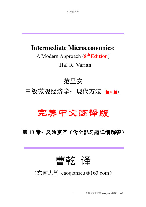
Fig.1.WealthandincomedistributioninIndia:(Left)Rankorderedwealthdistri-butionduringtheperiod2002-2004plottedonadouble-logarithmicscale,showingthewealthofthek-thrankedrichestperson(orhousehold)inIndiaagainsttherankk(withrank1correspondingtothewealthiestperson)aspersurveysconductedbyBusinessStandard[7]inDec31,2002(squares),Aug31,2003(triangles)andAug31,2004(circles).Thebrokenlinehavingaslopeof−1.23isshownforvisualreference.(Right)Cumulativeincomedistributionduringtheperiod1929-30asperinformationobtainedfromIncomeTaxandSuperTaxdatagiveninRef.[8].TheplothasGibbs/log-normalformatthelowerincomerange,andapowerlawtailwithParetoexponentα≃1.15forthehighestincomerange.
forthelow-incomeend,thedistributionfollowseitheralog-normal[4]orex-ponentialdistribution[5].Similarpowerlawtailshavebeenobservedforthewealthdistributionindifferentsocieties.Whilewealthandincomeareobvi-ouslynotindependentofeachother,theexactrelationbetweenthetwoisnotveryclear.Whilewealthisanalogoustovoltage,beingthenetvalueofassetsownedatagivenpointoftime,incomeisanalogoustocurrent,asitisthenetflowofwages,dividends,interestpayments,etc.overaperiodoftime.Ingeneral,ithasbeenobservedthatwealthismoreunequallydistributedthanincome.Therefore,theParetoexponentforwealthdistributionissmallerthanthatforincomedistribution.Mostoftheempiricalstudiesonincomeandwealthdistributionhavebeendoneforadvancedcapitalisteconomies,suchas,JapanandUSA.Itisinter-estingtonotethatsimilardistributionscanbeobservedevenforIndia[6],whichuntilrecentlyhadfollowedaplannedeconomy.AsincometaxandotherrecordsaboutindividualholdingsarenotpubliclyavailableinIndia,wehadtoresorttoindirectmethods.AsexplainedindetailinRef.[6],theParetoexponentforthepower-lawtailofthewealthdistributionwasdeterminedfromtherank-orderedplotofwealthoftherichestIndians[Fig.1(left)].ThisprocedureyieldedanaverageParetoexponentof≃1/1.23=0.82.AsimilarexercisecarriedoutfortheincomedistributioninthehighestincomerangeproducedaParetoexponentα≃1.51.Surprisingly,thisisidenticaltowhatParetohadthoughttobetheuniversalvalueofα.Comparingthiswithhistor-icaldataofincomedistributioninIndia[8],weagainobservethepower-lawTheRichAreDifferent!3tailalthoughwithadifferentexponent[Fig.1(right)].Inaddition,wenotethatthelow-incomerangehasalog-normalorGibbsformverysimilartowhathasbeenobservedforadvancedcapitalisteconomies[4].Inthesubse-quentsections,wewilltrytoreproducetheseobservedfeaturesofwealth&incomedistributionsthroughmodelsbelongingtothegeneralclassofassetexchangemodels.
2AssetexchangemodelsAssetexchangemodelsbelongtoaclassofsimplemodelsofaclosedeconomicsystem,wherethetotalwealthavailableforexchange,W,andthetotalnum-berofagents,N,tradingamongeachother,arefixed[9,10,11,12,13].EachagentihassomewealthWi(t)associatedwithitattimestept.Startingfromanarbitraryinitialdistributionofwealth(Wi(0),i=1,2,3,....),duringeachtimesteptworandomlychosenagentsiandjexchangewealth,subjecttotheconstraintthatthecombinedwealthofthetwoagentsisconservedbythetrade,andthatneitherofthetwohasnegativewealthafterthetrade(i.e.,debtisnotallowed).Ingeneral,oneoftheplayerswillgainandtheotherplayerwillloseasaresultofthetrade.Ifweconsideranarbitrarilychosenpairofagents(i,j)whotradeatatimestept,resultinginanetgainofwealthbyagenti,thenthechangeintheirwealthasaresultoftradingis:
Wi(t+1)=Wi(t)+∆W;Wj(t+1)=Wj(t)−∆W,where,∆Wisthenetwealthexchangedbetweenthetwoagents.Differentexchangemodelsaredefinedbasedonhow∆Wisrelatedto[Wi(t),Wj(t)].Fortherandomexchangemodel,thewealthexchangedisarandomfractionofthecombinedwealth[Wi(t)+Wj(t)],whileforthemin-imumexchangemodel,itisarandomfractionofthewealthofthepooreragent,i.e.,min[Wi(t),Wj(t)]].Theasymptoticdistributionfortheformerisexponential,whilethelattershowsacondensationoftheentirewealthWintothehandsofasingleagent[Fig.2(left)].Neitherofthesereflecttheem-piricallyobserveddistributionsofwealthinsociety,discussedintheprevioussection.Introducingsavingspropensityintheexchangemechanism,wherebyagentsdon’tputatstake(andarethereforeliabletolose)theirentirewealth,butputinreserveafractionoftheircurrentholdings,doesnotsignificantlychangethesteadystatedistribution[10].Byincreasingthesavingsfraction(i.e.,thefractionofwealthofanagentthatisnotbeingputatstakeduringatrade),oneobservesthatthesteady-statedistributionbecomesnon-monotonic,al-thoughthetailstilldecaysexponentially.However,randomlyassigningdiffer-entsavingsfractions(between[0,1])toagentsleadtoapower-lawtailintheasymptoticdistribution[13].ThisresultraisesthequestionofwhetheritisthedifferentialabilityofagentstosavethatgivesrisetotheParetodistribution.Or,turningthequestionaround,wemayaskwhethertherichsavemore.Thisquestionhasbeenthe