Use of the finite elements method for modelling the dynamic load impact on hydraulic leg equippe

合集下载

疲劳分析软件介绍_DesignLife_9-1_S2098-6_EN_web

Product Details
Streamlining the CAE Durability Process
Product Overview:
nCode DesignLife provides fatigue life prediction from finite element results to answer the question “how long will it last?” or “will it pass the test?” before you even have a prototype. Go beyond simplified stress analysis and avoid under- or over-designing your products by simulating actual loading conditions.
• Direct support for leading FEA results data including ANSYS, Nastran, Abaqus, LS-Dyna, RADIOSS and others
• Efficiently analyze large finite element models and complete usage schedules
• Crack Growth – provides a complete fracture mechanics capability using industry standard methodologies for specified locations on FE model. Built-in growth laws include NASGRO, Forman, Paris, Walker and more. Select from a provided library of geometries or supply custom stress intensity factors.

涂层中裂纹应力强度因子的计算及裂纹扩展

收稿日期:2007-03-12基金项目:国家自然科学基金资助项目(10472097).作者简介:覃森(1981-),男,重庆人,硕士研究生,主要从事材料失效的数值仿真研究.机械与材料涂层中裂纹应力强度因子的计算及裂纹扩展覃森,潘亦苏,罗征志(西南交通大学工程科学研究院,成都 610031)摘要:在涂层工作过程中,由于喷涂材料硬度高、抗裂性能差、喷涂工件刚性大工件表面产生应力集中,涂层很容易产生裂纹.对于含初始裂纹的喷涂材料,在拉伸载荷作用下裂纹的扩展与裂尖应力强度因子有很大的关系,根据断裂力学的基本原理,提出了利用数值模拟的方法来计算裂纹尖端的应力强度因子.并讨论了裂纹前沿网格划分对应力强度因子的影响,预测了裂纹扩展时形状的变化.关键词:三维有限元分析;应力强度因子;正交网格;裂纹扩展中图分类号:TH128 文献标识码:A文章编号:1671-0924(2007)06-0011-04Calculation of Crack Stress Intensity Factors andCrack Propagation in CoatingQIN Sen,P AN Y-i su,LUO Zheng -zhi(Research Ins titute of Engineering Science,Sou th west Jiaotong University,Chengdu 610031,China)Abstract:Because of the high hardness and lo w crack -resistance of spray material,and the high rigidity ofspray workpieces,and the stress convergence on the coating surface,cracks tend to result on the coating.To the initial spray material with a crack,the propagation path of the c rack in the material under tensile load has much to do with the stress intensity factor.According to the basic principle of the fracture me -chanics,this paper proposes the numerical method to calculate the stress intensity factor of the crack tip,discusses the effect of crack front grid partition on stress intensity,and predicts the shape changes during the propagation of crack.Key words:3-D FE M;stress intensity factors;orthogonal grid;propagation of crack0 引言从20世纪50年代初到60年代初断裂力学形成之后,就在航空航天、土木建筑及水利交通等众多领域中得以大力发展和广泛应用[1].断裂力学考虑材料破坏是由于初始裂纹的扩展造成的.在外力作用下,有初始裂纹的材料首先在裂纹尖端区域引起应力集中,所以裂纹在外力作用下就很容易引起扩展,直至裂纹失效.裂纹在外力作用下第21卷第6期Vol.21 No.6重庆工学院学报(自然科学版)Journal of Chongqing Institu te of Technology(Natural Science Edition)2007年6月Jun.2007应力强度因子对材料的破坏模式起非常重要的作用,所以受到众多研究者的重视.由于裂纹扩展和应力强度因子联系紧密,所以计算的应力强度因子的准确性对裂纹研究至关重要.数值模拟由于具有重复性好,费用低等优点,在该问题的研究中得到充分的应用,有限单元法、边界元法及位移不连续法等数值分析方法在裂纹模拟中得到了广泛应用[2-4].本文中采用有限单元法来计算涂层裂纹的应力强度因子,在此基础上使用Paris模型模拟裂纹扩展以及裂纹形状的变化.1 计算模型1.1 裂纹形状及扩展的基本假设1)裂纹相对结构中面是对称的,分析时只需取工件的四分之一来计算;2)裂纹面的形状呈半椭圆状,深度为a,长度为2c;3)基体和涂层间有好的界面连接;4)由于材料是线弹性的,假设裂纹的扩展方向沿裂纹线的法线方向.1.2 应力强度因子的计算方法对应力强度因子的精确估计可以降低在预测裂纹生长时的误差值,估计应力强度的方法有几种,其中有限单元法在计算复杂裂纹结构时由于其具有多功能性和普遍性而得到广泛应用.Hen-shell Shaw[5]和Barsoum[6]通过移动单元的中间节点到四分之一位置处来解决应力应变奇异性.在裂纹表面的四分之一处的应力强度因子可用下式估计:K=E4(1-v2)2r(1/4)u z(1/4)(1)其中:r(1/4)是四分之一处节点到裂尖的距离,uz(1/4)是四分之一处节点位置裂纹平面的偏离距离,E为弹性模量, 为泊松比.如图1所示.1.3 有限元建模喷涂材料采用的是镍铬硼硅型合金粉末,喷涂方法采用的是等离子喷涂法,喷涂所得涂层的弹性模量是120MPa,泊松比为0.3,本文中裂纹前沿采用20节点等参奇异单元,用四分之一节点来代替裂纹尖端节点,以适应该处的应力奇异.为研究裂纹前沿应力强度的影响因素,有限元模型按如下方法生成:为了方便建立模型和计算模型,把模型分为2个部分裂纹体模型和非裂纹体模型,在每步计算完成后,只需将裂纹体部分重新建模,而非裂纹体模型保持不变,这样可以节约大量的时间,裂纹体部分如图2所示.图1 裂尖附近的网格划分2 网格划分对应力强度因子的影响2.1 裂纹前沿非正交网格划分的影响当用四分之一节点位移方法来估计裂纹前沿应力强度因子时,裂纹前沿附近的网格划分对应力强度因子的计算有很大的影响.所得的应力强度因子或J积分值通过修正参数Y来确定,Y= J/( 2 a/E)或K/( a),裂纹前沿网格的划分如图3,计算得到的应力强度因子从图4中可以看出,随着网格前沿单元划分由垂直到偏离垂直, Y变化越来越大,最大误差达到25%,所以裂纹前沿网格的正交性对应力强度因子的影响非常大,划分网格时应避免过大地偏离正交.2.2 裂纹前沿奇异单元宽度与裂纹深度的比率的影响裂纹前沿的网格划分如图3所示,裂纹前沿奇异单元宽度L(如图1)与裂纹深度a的比值分别取0.02,0.04,0.08,0.12来研究,图4为裂纹前沿网格垂直度的影响、图5为裂纹前沿奇异单元长度与裂纹深度的比率的影响图,从图中可以看出,当比率小于0.1时,得到的应力强度因子差别不大,在误差范围内;当比率大于0.1时,裂纹前沿的应力强度因子变化很大.因此,本文中建议比率应小于0.1,此时应力强度因子计算较精确.12重庆工学院学报图2 裂纹体部分的有限元模型图图3裂纹前沿的网格划分图4 裂纹前沿网格垂直度的影响图5 裂纹前沿奇异单元长度与裂纹深度的比率的影响3 裂纹形状的改变涂层裂纹沿着深度和表面方向的生长用Paris 疲劳裂纹生长公式来估算:d a id N=C( K i )m (2)由式(2)可得:a i =K iK maxma max ,i =1,2(3)其中:m 是材料常数,对于大多数金属通常取2~4;i 是增量步; a max 是裂纹前沿最大应力强度因子处的裂纹生长增量.一旦有限单元计算成功完成,软件的后处理器开始工作.首先,它在每个裂尖位置从AB AQUS 输出文件中提取四分之一节点到裂尖的位移值和J 积分值(通常3个J 积分值可用).这些有限单元结果用四分之一节点位移和J 积分方法去计算裂纹前沿SIF 的变化.在每个位置取3个J 积分均值,并通过假设的应力或应变状态转变成SIF .在Paris 公式中通过选择合适的材料常数c 和13覃森,等:涂层中裂纹应力强度因子的计算及裂纹扩展m ,后处理器在裂纹前沿的角节点计算裂纹生长的法向增量和对应的疲劳循环增量.为了达到好的精度,裂纹前沿最大的生长增量 a max 通常取一个小值[7].后处理器自动地把裂纹前沿的角节点推进到一个新的位置,并用立方单元曲线方法重建一个新的裂纹前沿.这些新的节点(包括角节点和中间节点)沿着裂纹前沿被重新安排,以便于让他们有合适的距离.在新的节点被设置之后,在新的裂纹前沿软件产生了一个新的二维网格,并且在二维网格里重新布置所有的节点以使网格符合条件.以最初的半椭圆缺陷(a/c =0.5,Y 方向厚度为1m m)的裂纹一步步生长,弹性模量和泊松比在涂层、基体中分别是:70GPa,0.3;200GPa,0.3和18.6GPa,0.3.取m 的值为3,模型中大概有180个分析步,每12个分析步在图6和图7中被列出.可以看出,在裂纹的生长过程中,与最初的半椭圆形状相比,裂纹的形状改变越来越大,特别是最后阶段,顶部的接触载荷对裂纹形状产生越来越大的影响.当裂纹扩展靠近涂层顶部时,由于裂纹沿着厚度方向扩展越来越困难,当裂纹生长到涂层厚度的80%左右时计算终止.当基体强度为200GPa 时,裂纹沿x 方向扩展速率相对于基体强度为18.6GPa 时要小一些,即裂纹形状更趋于椭圆形扩展.图6 当基体弹性模量为18.6GPa 时裂纹形状的扩展图7 当基体弹性模量为200GPa 时裂纹形状的扩展4 结束语本文中描述了一种基于有限单元法计算涂层与基体间裂纹应力强度因子的方法,使用了一种裂纹前沿网格的划分形式,并讨论了2个重要参数:裂纹前沿网格的垂直划分和裂纹前沿奇异单元宽度与裂纹深度的比率对应力强度因子的影响,预测了裂纹扩展模式.按照本文中建立的含裂纹涂层的三维有限元模型进行分析,其结果与Newman -Raju 计算结果相对误差在可靠范围内,表明本文中采用的裂纹前沿垂直网格的划分方法的正确性.当选取裂纹前沿单元宽度与裂纹深度的比率大于0.1时,计算误差变得很大.涂层裂纹形状的扩展有一定的规律性,当裂纹扩展到涂层厚度的80%左右时,裂纹在厚度方向的生长很困难,此时,计算终止.本文中提供的三维有限元分析法不仅可以用来计算涂层裂纹的应力强度因子,还可以用来模拟各种复杂结构的裂纹及其形状的变化,为分析裂纹在工程中的应用提供了很好的解决方法.参考文献:[1] 范天佑.断裂理论基础[M ].北京:科学出版社,2003.[2] Sumi Y,Wang Z N.A finite2element simulation methodfor a system of growing cracks in a heterogeneous material [J].Mechanics of Materials,1998,28:197-206.[3] Sabhino D J,Trefftz.Boundary element method appliedtofracture mechanics [J].Engineering Fracture Mechanics,1999,16(4):485-492.[4] 黄醒春,顾隽超,夏小和.压载条件下裂纹断裂扩展的位移不连续数值分析[J].上海交通大学学报,2001,35(10):1486-1490.[5] Henshell R D,Shaw K G.Crack tip finite elements are un -necessary[J].Int J Numer Meth En gng,1975,9:495-507.[6] Barsoum R S.On the use of isoparametric finite elements inlinear fracture mechanics [J].Int J Numer MethEngng 1976,10:25-37.[7] Lin X B,Smi th R A.Finite element modelling of fatiguecrack growth of surface cracked plates[J].The numerical technique,2000(5):43-45.(责任编辑陈松)14重庆工学院学报。

小型货车钢板弹簧结构有限元仿真设计毕业论

摘要钢板弹簧具有结构简单、工作可靠、价格低廉等优点，在汽车中被广泛地使用。

它在工作过程中存在大变形、叶片间的接触等多种非线性因素，故多年来一直没有形成一个比较切合实际的完善的设计与分析方法。

集中载荷法、共同曲率法等传统设计方法以线弹性理论为依据，把问题抽象为简单的数学、力学模型，并应用材料力学公式进行粗略计算，一般计算结果与实际情况差别较大。

随着汽车向轻量化和高速化发展，对悬架的要求越来越高。

显然，传统设计方法已经不能适应现代汽车发展对悬架的要求。

近年来，随着有限元技术、CAE技术的不断发展以及在工程中的成功应用，以计算机为工具、有限元分析为基础的CAE法正逐渐成为汽车设计的主流。

应用CAE法进行钢板弹簧设计可以同时考虑到结构的大变形、摩擦、簧片间的接触以及组装时的预应力和工作应力的结合，从而实现对钢板弹簧的精确设计。

本文根据汽车设计的要求对悬架中的钢板弹簧进行了设计和计算，并使用UG进行建模，然后应用ABAQUS有限元分析软件进行了受力分析和仿真设计和计算。

关键词：钢板弹簧 ABAQUS 有限元Jubilee wagon spring structure finite element simulationdesignABSTRACTThe spring has the structure simply, the work reliable, the price inexpensive and so on the merits, widely is used in the automobile. It has contact between the big distortion, leaf blade's in the work process and so on many kinds of non-linear factors, therefore for many years has not formed of a quite realistic perfect design and the analysis method. Traditional design methods and so on concentrated load law, common curvature law take the line theory of elasticity as the bases, abstracts the question as the simple mathematics, mechanics model, and carries on the rapid calculation using the materials mechanics formula, the general computed result and the actual situation difference are big. Along with the automobile to the lightweight and the high speed development, is more and more high to the suspension fork request. Obviously, the traditional design method already could not adapt the modern automobile development to the suspension fork request.In recent years, along with the finite element technology, the CAE technology unceasing development as well as in the project success application,take the computer as the tool, the finite element analysis was becoming the automobile design gradually for the foundation CAE law the mainstream.Carries on the spring design using the CAE law to be possible simultaneously to consider the structure the bigdistortion ,contact as well as assembly between friction, time reed pre-stressed and working stress union, thus realizes to the spring precise design.This article according to the automobile design the request to carry on the design and the computation to in the suspension fork spring, and used UG to carry on the modelling, then has carried on the stress analysis and the simulation design and the computation using the ABAQUS finite element analysis software.Key words: leaf spring, ABAQUS, finite element小型货车钢板弹簧结构有限元仿真设计龚顺聪 0611032680 引言钢板弹簧几何形状简单，传统计算方法应用梁理论，简单地看是合理的，实际上远不如此。

SESAM软件GeniE建模自学手册

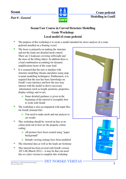
SesamPart 0 - GeneralCrane pedestal Modelling in GeniESesam User Course in Curved Structure Modelling Genie Workshop: Local model of crane pedestal• •The purpose of this workshop is to create a model intended for stress analysis of a crane pedestal installed on a floating vessel. The focus is primarily on making the structure and not the loads nor detailed mesh control. There are 2 loadcases covering selfweight and the mass of the lifting object. In addition there is a load combination accounting for dynamic amplification factor of the crane load. It is assumed that the user is familiar with structure modelling (beams and plates using snap to point modelling techniques). Furthermore, it is required that the user has basic knowledge on GeniE’s user interface and how the user may interact with the model to derive necessary information (such as length, positions, properties, display settings and so on). Some detailed guidance is given in the beginning of the tutorial to exemplify how to work with GeniE••The workshop is also accompanied with input files for GeniE (Journal file) You need to make mesh and run analysis to see results•This workshop should be viewed on-line or on colour print out to best see the property colour coding. All pictures have been created using “paper background” Default viewing settings have been modified• •The structural data as well as the loads are fictitious This tutorial has been revised with GeniE version D5.3-06 (March 2011) – it may be that you need this or a later version to complete this workshopDNV Software – GeniE Crane Pedestal Workshop Revised 12 March 2011DET NORSKE VERITAS1SesamPart 0 - GeneralCrane pedestal Modelling in GeniE• • • •Part 0 – General introduction to the workshop Pages 1-3 Part 1 – Design premise Define the units, material and section types Pages 4-10 Part 2 – Guiding geometry Define the guiding geometry needed to define the outer hull and deck levels Pages 11-13 Part 3 – Make the outer hull Model the hull interactively. You will se the 1 2 symbols to the right that represent start and stop of beams during modelling. Click start of beam Click end of beam Notice that the symbol for right mouse bottom click is different from left mouse bottom click Use right mouse button Pages 14 - 18 3 Part 4 – Make the deck plates sensitive menu Create the deck levels and insert stiffening in between using both plates and beams Pages 19 – 27 Part 5 – Make the column Insert the column between lower deck and above upper deck level Pages 28 – 32 Part 6 – Create the web frames Insert three simple web frames and connect to the Pages 33 – 34 Part 7 – Column stiffening Insert vertical stiffeners as well as a ring stiffener at top of column Pages 35 – 38 Part 8 – The crane Model the crane using beams in order to apply the loads at end of crane tip Pages 39 – 43 Part 9 – Boundary conditions Insert pinned boundary conditions along all free edges and ensure that the simplified crane beam is connected properly to the shell column model by using linear dependencies Pages 44 – 45 Part 10 – Loads Create one loadcase with selfweight, another with 75 tonnes load at the crane tip and a load combination where loadfactor 1.6 is used on the crane load Pages 46 – 48to activate the context• • • • • ••DNV Software – GeniE Crane Pedestal Workshop Revised 12 March 2011DET NORSKE VERITAS2SesamPart 0 - GeneralCrane pedestal Modelling in GeniE• •Part 11 – Verify model Verify the model before launching the analysis, Page 49 Part 12 – Run analysis Run the analysis and see how the mesh and results changes when performing changes in the global mesh settings. Learn how to work with sets in results presentation and open the results in Xtract Pages 50 -57DNV Software – GeniE Crane Pedestal Workshop Revised 12 March 2011DET NORSKE VERITAS3SesamPart 1 – Design premiseCrane pedestal Modelling in GeniE•Define units meters and N Start the program and open a new workspace File|New Workspace. Specify name Crane_pedestal_tutorial and use the default values for database units. Click OK when done. » Notice, if you want Finite Element results in other units than N and m, you need to change now.•Define materials Use the command Edit|Properties and select Material. Select Create/Edit Material to give the details for MAT1 (remember to tick “Allow edit”). Set the material type to default and click OK when doneDNV Software – GeniE Crane Pedestal Workshop Revised 12 March 2011DET NORSKE VERITAS4SesamPart 1 – Design premiseCrane pedestal Modelling in GeniE•Define section properties Section profiles Tbar425x120x12x25, Tbar575x150x12x25 and Tbar885x200x14x35 are found from section libraries Section profiles (user defined name) Column, Crane_inner, Crane_outer and Hydraulic_cylinder are defined by the user Use the command Edit|Properties and select Section. Select Create/Edit section to start defining the sections. Select “Section Library”Find the right section library from “Browse” and select the library ‘tbar’ (a library containing typical Tbar ship profiles)DNV Software – GeniE Crane Pedestal Workshop Revised 12 March 2011DET NORSKE VERITAS5SesamPart 1 – Design premiseCrane pedestal Modelling in GeniEYou may find the profiles Tbar425x120x12x25, Tbar575x150x12x25 and Tbar885x200x14x35 The sections are now selected by clicking on Tbar425x120x12x25 and then RMB+click on Tbar575x150x12x25 and Tbar885x200x14x35 » The picture below shows the selection of Tbar425x120x12x25 and Tbar575x150x12x25 Click OK and the profiles are now part of the design premiseClick create/edit section to define the remaining profilesDNV Software – GeniE Crane Pedestal Workshop Revised 12 March 2011DET NORSKE VERITAS6SesamPart 1 – Design premiseCrane pedestal Modelling in GeniEDefine the profiles Column, Crane_inner, Crane_outer and Hydraulic_cylinder as shown below. You may use mixed units as shownDNV Software – GeniE Crane Pedestal Workshop Revised 12 March 2011DET NORSKE VERITAS7SesamPart 1 – Design premiseCrane pedestal Modelling in GeniE•Define the plate thicknesses Pl12, Pl15 and Pl30 as follows: Use the command Edit|Properties and select Thickness. Select Create/Edit Thickness to start defining the thickness propertiesDNV Software – GeniE Crane Pedestal Workshop Revised 12 March 2011DET NORSKE VERITAS8SesamPart 1 – Design premiseCrane pedestal Modelling in GeniE•The thickness and section properties may now be accessed from the browser. Since the modelling will start with the outer hull, the plate thickness Pl15 should be set as default. Similarly, the first use of stiffeners will be at a deck level; you should set Tbar885x200x14x35 to defaults. Notice also the default symbol that will appear. Material default has already been set when creating the property1Use right mouse button to activate the context sensitive menu1Use right mouse button to activate the context sensitive menuDNV Software – GeniE Crane Pedestal Workshop Revised 12 March 2011DET NORSKE VERITAS9SesamPart 1 – Design premiseCrane pedestal Modelling in GeniE•Specify the mesh settings for automatic mesh creation as follows: Edit|Rules|MeshingDNV Software – GeniE Crane Pedestal Workshop Revised 12 March 2011DET NORSKE VERITAS1010 in each direction (equal length of allD ET N ORSKE V ERITASD ET N ORSKE V ERITASSelect GuidePlane2 and copy to the other side of GuidePlane1.1Select guideplaneUse right mouse button2to activate the contextsensitive menu3Select copy4Click startof copy vector5Click endof copy vector6Perform copyoperationD ET N ORSKE V ERITASD ET N ORSKE V ERITASInsert two guidelines as follows:Insert|Guiding Geometry|Guide Line DialogBefore accepting above dialog,change z-coordinate for end point to 0.5 mStart line1Find start point2End line3Find end point4Edit the lowest point and change z-coordinate from 2m to 2.5 mLine Dialog2Find end point1Find start pointD ET ERITASJoin Curve1 and Curve2 by using the fillet curve option» 4. Change radius to 2.5 by typing 2.5 andclick <Enter>» 5. The two curves (1&2) are now joinedto a composite guide curve, Curve3D ET N ORSKE V ERITASCopy Curve3 to the other end of the bottom guideplane as follows:2. Right click to activate the menu copy5Performcopy3Find start point4Find end pointD ET N ORSKE V ERITAS» 4. Click on Curve 4 again to stop skinning operation and the hull plate is created having thickness 15mm since this was the default setting •In case you had several curves click on each one sequentially and double-click on final curveV ERITASD ET N ORSKE V ERITASCreate the horizontal deck levels at elevations 2m, 5m, 7m, 11m, 14m and 15m. The steps are:1. Change default thickness value toPl12. Right click Pl12 in the Thickness browser and select Set Default2. Insert the top plate by clicking thefour plate corners as shown below. Use command Insert|Plate|Flat Plate Dialog orFirst corner1Second corner2Third corner3Fourth corner4Above using ”Default display”Right using ”Modelling –Structure”D ET N ORSKE V ERITAS3. Copy Plate2 downwards to the other levels, also for elevation 2m. Find the copy»Click Copy Translate »Click from position »Click to position»Picture to right shows copy toelevation 11m»Use same copy technique and create plates at elevations 7m, 5m and 2m»Notice for 2 meters use the same plate even though it is outside the hull. The plate will be trimmed in the next operationUse right mouse button to activate the context sensitive menu2From3To4SesamPart 4 – Make the deck plates4. Trim Plate Pl7 so that it matches the hull form. » Select the plate, RMB and select DivideCrane pedestal Modelling in GeniE»The plate is now divided in two parts – the split is along the intersection with the hull. Select the outer part of the horizontal elevation and delete it.DNV Software – GeniE Crane Pedestal Workshop Revised 12 March 2011DET NORSKE VERITAS21SesamPart 4 – Make the deck platesCrane pedestal Modelling in GeniE5. Make the stiffening between plates at elevation 14m and 15m » Copy GuidePlane1 to elevations 14m and 15m » Insert a vertical plate using the highlighted positions as the four plate corner points 5 spacings» »Select the new plate, RMB and click Copy Translate Specify copy vector 1.4 m in x-direction and copy 3 timesDNV Software – GeniE Crane Pedestal Workshop Revised 12 March 2011DET NORSKE VERITAS22SesamPart 4 – Make the deck plates» Repeat copy operation, but use vector (-1.4m, 0m, 0m)Crane pedestal Modelling in GeniE»Select all the new vertical stiffening plates, RMB and click Copy Rotate • Rotate around position (5m, 5m, 15m) which is the centre of the plate (and also centre of the column to be modelled)Structural parts hidden for better visibilityDNV Software – GeniE Crane Pedestal Workshop Revised 12 March 2011DET NORSKE VERITAS23SesamPart 4 – Make the deck platesCrane pedestal Modelling in GeniE6. Make the vertical plates between lowest deck level and the hull. The steps are: » Copy GuidePlane1 to deck elevation 2m » Insert vertical plates at same positions as for the upper deck. Use same modelling procedure by inserting one plate and copy in positive and negative x-direction. Select all plates and rotate as on previous page» »Select all new vertical plates, RMB and click Divide Delete all plate parts outside the hull.DNV Software – GeniE Crane Pedestal Workshop Revised 12 March 2011DET NORSKE VERITAS24SesamPart 4 – Make the deck platesCrane pedestal Modelling in GeniE7. For the remaining deck levels insert vertical stiffening using beams. Follow the steps: » Set section property Tbar885x200x14x35 to default » The stiffeners shall be inserted at the same locations as the vertical stiffener plates (see previous pages). » Copy GuidePlane1 to elevation 11 m and use as reference. » Insert one stiffener at elevation 11m (Insert|Beam|Straight Beam)2To1From»Flush the stiffener to the plate elevation, flush top if it is like the one on the picture shown below. If its opposite of this one, rotate and flush bottom.3RMBDNV Software – GeniE Crane Pedestal Workshop Revised 12 March 2011DET NORSKE VERITAS25SesamPart 4 – Make the deck plates»Crane pedestal Modelling in GeniESelect the stiffener and copy in positive and negative x-direction as follows»Select all stiffeners, RMB and click Copy Rotate • Rotate around position (5m, 5m, 11m)DNV Software – GeniE Crane Pedestal Workshop Revised 12 March 2011DET NORSKE VERITAS26SesamPart 4 – Make the deck plates»Crane pedestal Modelling in GeniESelect all stiffeners and copy to the deck elevations below:1From2To1From2ToDNV Software – GeniE Crane Pedestal Workshop Revised 12 March 2011DET NORSKE VERITAS27SesamPart 5 – Make the columnCrane pedestal Modelling in GeniE•The steps are as follows 1. Select the top guideplane (GuidePlane5) and hide all other structure or guiding geometries. Right click the guideplane, click Visible Model and select Show selection only (or use ALT+S)2. Look at the guideplane from top – rotate the guideplane or use tool button “View from Z” or (F8)3. Make a curved guideline forming one quarter of the column circle » Insert points for the curve first (Insert|Guiding Geometry|Guide Point Dialog) » Use points to create the guide21FromOrigin3ToDNV Software – GeniE Crane Pedestal Workshop Revised 12 March 2011DET NORSKE VERITAS28SesamPart 5 – Make the column4. Copy the guide curve to elevations 5m and 20m » I.e. copy vectors (0,0,-10) and (0,0,5) 5. Copy and rotate the selected guidecurves -90 degreesCrane pedestal Modelling in GeniE6. Select the guide curve highlighted above and move to the deck level below at elevation 2m, i.e. a copy vector (0,0-3) 7. Set default plate thickness to Pl30DNV Software – GeniE Crane Pedestal Workshop Revised 12 March 2011DET NORSKE VERITAS29SesamPart 5 – Make the columnCrane pedestal Modelling in GeniE8. Make the column plates by a skin operation between the relevant curves. Remember to double click the end curve to finalise the skin command » Make two quart parts and copy mirror theseDNV Software – GeniE Crane Pedestal Workshop Revised 12 March 2011DET NORSKE VERITAS309. Insert a vertical plate between deck levels 2m and 5m below the column»Delete the highlighted beam»Set plate thickness Pl12 to default»Insert the plateD ET N ORSKE V ERITASRemember to deactivate the Paintbrush tool button by clickingD ET N ORSKE V ERITASD ET N ORSKE V ERITAS•This part shows how to create three web frames. The procedure is as follows:1. View the model from one side and make sureyou see the vertical guideplane. Select the guideplane and show this only2. Insert the web frame by using insert flat plateand snap point loop. Click the plate corners on the guideplane as shown, remember to close the loop by finally clicking on the start point again.3. Select the web frame, RMB and divide it.Trim the plate to the hull by deleting the part outside the hull1st corner 12nd corner23rd corner34565. Move and copy the web frame to final positions»Move to intersect with first occurrence of stiffenerERITAS4. Insert stiffeners by using command Insert|Beam|Straight Beam Dialog. Click on bottom point and edit the upper point so that the z—coordinate becomes 5m+15m (or 20m)»Select the beam, RMB, Edit Beamand offset the beamD ET N ORSKE ERITAS6. Select all the 4 stiffeners and rotate 3 times using 90 degreesRotate around column centre lineD ET N ORSKE V ERITAS7. Insert the top ring stiffener by using Insert Beam|Curved BeamSet section property Tbar575x150x12x25 to defaultInsert the beam by clicking the start point and double»Select the beam, RMB and align beam local axis to column plate »Flip the beam so that flange is on inside 132Click on column plateD ET N V»Copy rotate the stiffener 3 times using 90 degrees •Column centre line as rotation axisV ERITAS3. Insert the crane beam by Insert|Beam|Straight Beam Dialog. Find the start point by clicking on the reference point defined by the two guide lines above. Edit the end point as shown below (z-elevation 33m)»Notice that the cranebeam is modelled as a beamand not a plateORSKE V ERITAS»Select the upper beam and divide using parameter 4/6D NSesamPart 8 – The crane5. Create the crane cantilever » Set section property Crane_inner to default » Use command Insert|Beam|Straight Beam Dialog to create the beam. • Start point is at elevation +27 m • End point is edited as shown belowCrane pedestal Modelling in GeniE»Double click the horizontal beam and make segments with Right click|Divide as follows:DNV Software – GeniE Crane Pedestal Workshop Revised 12 March 2011DET NORSKE VERITAS41SesamPart 8 – The crane»Crane pedestal Modelling in GeniESelect the segment to the left and change section property to Crane_outer • RMB to activate the commands • Double click in graphic window to exit segmented modelling view»Move the segmented beam upwards 4 meters. Select the beam, RMB and MoveDNV Software – GeniE Crane Pedestal Workshop Revised 12 March 2011DET NORSKE VERITAS42SesamPart 8 – The crane»Crane pedestal Modelling in GeniESelect the segmented beam and move the end 2 m upwards • RMB, Edit Beam and Move end2P21P16.Insert the hydraulic cylinder » Set section property Hydraulic_cylinder to default » Insert the beam by clicking between points P1 and P2 as shown aboveDNV Software – GeniE Crane Pedestal Workshop Revised 12 March 2011DET NORSKE VERITAS43SesamPart 9 – Boundary conditionsCrane pedestal Modelling in GeniE•The boundary conditions along plate members are assumed to be /fixed, fixed, fixed, free, free, free) Ensure there are guide lines along all relevant edges Select the edges and click “Create Support Curve” » You may also insert support curves by using Remember to double click the end point Select the Support Curves, RMB, Properties and change from fixed in all dof’s to (fix, fix, fix, free, free, free)DNV Software – GeniE Crane Pedestal Workshop Revised 12 March 2011DET NORSKE VERITAS44SesamPart 9 – Boundary conditionsCrane pedestal Modelling in GeniE•Connect the top of the shell column to the lower part of the beam column and ensure plane sections remain plane Use a support rigid link Step 1: Select the independent point » The bottom point of the crane beam Step 2: Decide boundary conditions for independent point » Free in all degrees of freedom, i.e. free to move and rotate Step 3: Decide dependent region » Centre of volume is in the middle of the column (i.e. same as the independent point) » Ensure that all edges of the shell circle is part of region, use dx=6m, dy=6m, dz=0.2m)The symbols for the rigid support link looks like:DNV Software – GeniE Crane Pedestal Workshop Revised 12 March 2011DET NORSKE VERITAS45SesamPart 10 – LoadsCrane pedestal Modelling in GeniE•Before making the loadcases make an analysis activity Right click in right browser pane area to access the commands Specify activity name Linear_static•Make two loadcases to represent the structure selfweight and the crane load Create the loadcases from the browser pane area as shownDNV Software – GeniE Crane Pedestal Workshop Revised 12 March 2011DET NORSKE VERITAS46SesamPart 10 – LoadsCrane pedestal Modelling in GeniE•Include selfweight in LC1_stru Select the laodcase, RMB and choose Properties. Tick for ”Include structure selfweight in structural analysis”•Ensure that LC2_cran is the active loadcase by selecting the loadcase, RMB and choose Set CurrentDNV Software – GeniE Crane Pedestal Workshop Revised 12 March 2011DET NORSKE VERITAS47SesamPart 10 – LoadsCrane pedestal Modelling in GeniE•Include a point load at the crane tip equal to 75 tonnes x gravity ≈ 750.000 N Insert|Explicit Load|Point Load•Make a loadcombination LC3_comb and use load factor 1.6 on LC2_cranDNV Software – GeniE Crane Pedestal Workshop Revised 12 March 2011DET NORSKE VERITAS48SesamPart 11 – Verify modelCrane pedestal Modelling in GeniE•Run Tools | Structure | Verify to verify the model before launching the analysis. The model verification should indicate that there are two disjoint model parts, but this is due to the program not treating the rigid support link as geometry. The analysis will run.If no other warnings or problems are reported, you can continue to the next page to run the analysis.DNV Software – GeniE Crane Pedestal Workshop Revised 12 March 2011DET NORSKE VERITAS49SesamPart 12 – Run analysisCrane pedestal Modelling in GeniE•Run the analysis from Tools|Analysis|Activity Monitor (or by using the shortcut ALT+D) There are several ways of verifying analysis details. The example below shows how to open the listing file from the analysis done by Sestra•You may now look at the finite element mesh and results by selecting e.g. the view setting “Results with mesh” It is not the objective of this tutorial to do results presentation, but the results are accessed as follows or from using short-cut ALT+P (in this case the displacements are shown for the whole structure using load combination LC_comb) The mesh is also very coarse since no mesh details have been specifiedDNV Software – GeniE Crane Pedestal Workshop Revised 12 March 2011DET NORSKE VERITAS50。

法国电网电能质量承诺和电能质量评估_英文_

2009年第3卷第3期南方电网技术特约专稿2009，V ol. 3，No. 3 SOUTHERN POWER SYSTEM TECHNOLOGY FeaturedArticles 文章编号：1674-0629(2009)03-0007-08 中图分类号：TM934.5 文献标志码：A 法国电网电能质量承诺和电能质量评估杨显军（法国电力公司研究与开发部，92141 卡拉马特，法国）摘要：介绍法国电网的电能质量承诺，包括输电运营商（TSO）的质量承诺和配电运营商（DSO）的质量承诺。

TSO和DSO在作出电能质量承诺的同时，还利用入网规则以协议的方式来考虑和限制每个客户的负荷和分布式电源对电能质量的影响。

这些协议的实施表明，只有遵守承诺，加上电网运营商与用户双方共同作出努力，才能获得全面良好的电能质量。

对于电网干扰评估，建议使用基波潮流计算与多相谐波注入相结合的方法。

这个方法利用很短的计算时间就能对非线性负荷建模情形给出可接受的结果。

所提议的频域方法的要点在于，将每个谐波源逐一地同时作为扰动源和受扰者来考察，以便计及扰动源之间的相互作用。

研发了一个即插即用的HVDC组件并将其用在文章最后部分实例研究中。

关键词：电能质量承诺；频域建模；谐波；电力电子设备；高压直流输电Grid Power Quality Commitments and Grid Power Quality Assessmentin FranceYANG Xian-jun (Xavier X. YANG)(R&D, Electricité de France, 92141 Clamart, France)Abstract: Grid Power Quality Commitments in France are introduced, including the Power Quality Commitments of TransmissionSystem Operator (TSO) and the Power Quality Commitments of Distribution System Operator (DSO). Undertaking the commitments,TSO and DSO are using connection rules to take into account and minimize the impact on power quality of each customer (load ordistributed generation) in the way of contracts. The practice of these contracts shows that a good overall power quality can only beachieved by respecting commitments and doing effort from both of grid and customer sides. For grid disturbance assessment, it issuggested to use multi-phase harmonic injection method with fundamental power flow. This method can give an acceptable resultswith very short computing time for non-linear load modelling. The key point of proposed frequency domain method is that eachharmonic source is individually considered as both disturbance source and disturbance receiver in order to take into accountinteractions between sources. A plug & play HVDC component has been developed and used in one of two case-studies in the end ofthis article.Key words: power quality commitment; frequency domain modelling; harmonic; power electronic device; HVDC1 Power Quality Commitments1.1 Power Quality Contracts and CommitmentsStandard EN 50160 gives the main voltage pa-rameters and their permissible deviation ranges at the point of common coupling (PCC) in public low volt-age (LV) and medium voltage (MV) electricity distri-bution systems, under normal operating conditions.Based on EN 50160 and the former French power quality contract Emeraude, two new grid access con-tracts have been put into service in France between system operators (utilities) and customers: called CART for transmission customers and CARD for dis-tribution customers, see Fig. 1. These contracts not only set the power quality commitments for the grid operators but also for the customer disturbance emis-sion level.Fig. 1 Power Quality Commitments in CARD and CART8南方电网技术第3卷The power quality that is handled in grid access contracts includes harmonic, unbalance, flicker, inter-ruption, voltage dip disturbances. Among these dis-turbances, the number of interruption is considered as commitment and others are given as indicative values. 1.2 Power Quality Commitments of Transmis-sion System Operator (TSO)French TSO has the standard and personalized contractual commitments with the customers concern-ing:1） long interruptions (1 per year, 2 per 3 years, 1 per 3 years)；2） short interruptions (1 to 5 per year, 1 to 2 per 3 years)；3） voltage dips (optional from 3 to 5 per year)； 4） RMS voltage magnitude (± 8 %)； 5） frequency (± 1 %)； 6） voltage unbalance (< 2 %)； 7） harmonics ；8） rapid voltage fluctuations, flicker (P lt < 1). For transmission power supply voltage, harmonic limits have been set (Tab. 1). These limits are meas-ured by 10 min mean value at each harmonic voltage (h ≤ 25, the order of harmonics) and total harmonic distortion (THD , h ≤ 40) during 100% of time. For transmission customer, current harmonic emissions are also limited in % compared to contracted rated currenth HRU lim /%h HRU lim /%h HRU lim /%5, 7 2.0 3 2.0 2 1.5 6.0 11, 13 1.5 9 1.0 4 1.0 6.0 171.015, 210.5> 40.56.019 1.0 6.0 23, 25 0.76.01.3 Power Quality Commitments of DistributionSystem Operator (DSO)The Tab. 3 shows the contracted voltage interrup-tion values for the four geographical zones.With personalized contracts signed jointly by system operators and customers, it is possible to in-clude some voltage dips in guaranteed power supply quality by network operators.Tab. 2 Transmission Customer Current Harmonic Commitments Odd Order hHRI lim /% Even Oder h HRI lim /%3 4.0 2 2 5, 7 5.04 1.0 9 2.0 > 4 0.5 11, 133.0>13 2.0Tab. 3 DSO Commitments of Voltage Interruptions per Year Interruption DurationZone 1 Zone 2 Zone 3Zone 4≥ 3 min6 3 3 2 > 1 s and < 3 min301032As grid commitments (Tab. 4), harmonic limits have been set for distribution power supply voltage. These limits are measured by 10 min mean value ateach harmonic voltage (h ≤ 25) and total harmonic distortion (THD , h ≤ 40) during 100% of time. For distribution customer, current harmonic emissions are also limited in % compared to contracted rated current (Tab. 5).Tab. 4 Distribution Voltage Harmonic Commitments Odd Harmonic OrderNot-Triplet Triplet Even HarmonicOrderTHD lim /13 3.0 8.0 17 2.0 8.0 19, 23, 251.5 8.0Tab. 5 Distribution Customer Current Harmonic Commitments Odd Order hHRI lim /% Even Oder h HRI lim /%3 4.0 2 2.0 5, 7 5.04 1.0 9 2.0 > 4 0.5 11, 133.0>13 2.0第3期杨显军：法国电网电能质量承诺和电能质量评估 9For more detail of the power qualify commit-ments of TSO and DSO, please see the following web site: /.1.4 Customer Load ConnectionIn order to meet their power quality commitments, TSO and DSO are using connection rules to take into account and minimize the impact on power quality of each customer (load or distributed generation). DSO has set up a number of technical referential documents and studying tools for load connection. Before per-forming a load or a DG connection, DSO undertakes three level’s studies which are based on standards and site measurements. The aim is to anticipate the possi-ble disturbances which may be provoked by the equipment to be connected and to determine the most adaptive Point of Common Coupling (PCC). Follow-ing these steps, DSO can ensure the optimal perform-ance of the network for all users.The first level study includes identifying the main characteristics of the installation to be connected and effectuating a global analysis. The second level con-sists of evaluating particularly the disturbances. The third level is composed of a detailed study on the iden-tified disturbances. In wind mill connection, this study is based on the standard IEC 61400-21 which evalu-ates the impact in terms of power quality [1].1.5 Power Quality Indices and Evolution ofCommitmentsIn order to measure the evolution of power qual-ity, DSO calculates a number of criterions based on network parameters. These indicators make it possible to evaluate the needs of power supply infrastructure improvement. The following values have been defined as power quality indicators:1）SAIDI or B-Criterion in France, index of mean duration of interruption for LV customers;2）SAIDI for MV customers weighted by the supplied power;3）SAIFI, indices of mean number of interrup-tion of the network, for the long interruption (t id > 3 min), the short interruption (1 s≤ t id≤ 3 min) and the very short interruption (t id < 1 s) . 2 Harmonic Source Modelling and GridDisturbance Assessment2.1 Simulation MethodFrequency domain analysis uses an admittance matrix system model developed from individual com-ponent level models connected according to system topology. The development of admittance matrix mod-els is based on multi-port network theory. Linear grid components are similarly developed from multi-port admittance parameters.In frequency domain simulation, harmonic gener-ating devices are usually modelled by current sources and the whole system admittance matrix is resolved from a start frequency to an end frequency with a fixed or variable frequency step. The deficiencies in the current source method can be partially overcome using a technique that has come to be known as “harmonic power flow”. More often, a fundamental frequency power flow solution is executed using a linear model for all power delivery equipment and loads, and the resultant fundamental frequency load terminal volt-ages are used to “adjust” non-linear load harmonic current vectors automatically without additional user action. However, in frequency approach, initial har-monic current patterns are still required to be known for each nonlinear load.2.2 Harmonic Source ModellingHarmonic model based on a constant current source, see Fig. 2(a), can’t represent real harmonic currents generated by a power electronic device con-nected to an actual network.Fig. 2 General Structure of Three Phase Harmonic Source ModelThe method (a) is too simplified because actual harmonic current of an electric device is always con-10南方电网技术第3卷trolled by network configuration. In order to overcome this drawback, we have developed multiphase har-monic model with a voltage vector controlled current source and a frequency-variable impedance to repre-sent an actual harmonic source, see Fig. 2(b). In pro-posed method (b), J (f ) is a current source controlled by the fundamental voltage crossing frequency-variable impedance Z (f ). Z (f ) represents the behaviour of the power electronic device towards harmonic distur-bances coming from power supply side.The method (b) is detailed in the following para-graphs.Equivalent harmonic current source of a nonlin-ear load is generated by two main steps: the initial cur-rent J 0(f ) and the corrected current source J (f ) by load-flow. In parameter setting before simulation, the initial J 0(f ) is defined by pre-designed waveform pat-tern, rated power and rated voltage of the load. In fre-quency domain, J 0(f ) is represented by the followingformula:00()()cos()k kJ f J k k t ωφ=⋅+.The pre-designed waveform patterns include cur-rent waveforms generated by the most usual distur-bance sources such as 6-pulse and 12-pulse rectifiers, dimmers, arc furnaces, etc. The following procedure summarizes the proposed source modelling method:1） Choosing a pre-designed waveform (database, analytical formulas, wave form generated by Excel data sheet, empirical data table, on-site measurements) which represents the current harmonic distortion to be used;2） Refining the waveform by particular working state of the device. For example, by switching angle of rectifier and by short-circuit power of upstream net-work;3） Spectrum calculation of the refined wave-form by means of Fast Fourier Transform;4） Calculation of the designed fundamental current and phase angle between voltage and current from rated electric values of the device: voltage, pow-ers P and Q ;5） Pre-design of the harmonic spectrum at rated current and creation of a voltage controlled current source model for frequency domain simulation J 0(f ), see example in Fig. 3 for the used current pattern of a 12-pulse rectifier.Fig. 3 Current Waveform and Harmonic Spectrumof a 12-Pulse RectifierDefine the source impedance Z (f ) as a function of frequency. Z (f ) reflects the device behaviour to the disturbances coming from power supply side.For particular case, it is very important to define Z (f ) values within the studied frequencies. For instance, a static converter’s impedance was set an infinite value in the past in performing inter-harmonic studies. This is not true for a number of static converters. Some in-dustrial cases show the ripple control signal at 175 Hz can be partially absorbed by a rectifier with a capacitor filter as in a variable-speed drive [2].The proposed harmonic source model behaviours as follows: when the source J (f ) is activated, imped-ance Z (f ) is naturally set to an infinite value because the device behaviours as a current source. When the source J (f ) is not activated, Z (f ) has to be added into the system admittance matrix. In this case, the device behaviours as a passive component. Value of Z (f ) is defined case by case in accordance with studied phe-nomena:At fundamental frequency, Z (f ) is calculated from rated voltage and powers P , Q of the simulated device.第3期杨显军：法国电网电能质量承诺和电能质量评估 11At studied harmonic or inter harmonic frequen-cies whose source comes from the power supply side, Z(f) can be defined from the real response of the de-vice at these frequencies. Z(f) is depending on device structure, it can be modelled by series (or parallel) RL, RC circuits, by mixed model of CIGRE 36.05[3] or by a data table for irregular cases.If it is difficult to define a general analytical for-mula representing Z(f) for all studied frequencies. For studying a specific frequency, a simple solution is to perform a time domain simulation on the power elec-tronic device in order to obtain the impedance re-sponse. For example, at ripple control frequency of 175 Hz, the equivalent impedance at input of a recti-fier changes with the type of the rectifier structure, DC bus filter, AC filter and rectifier control techniques. A time domain simulation shows that for a 400 V, 250 kV A diode rectifier used in a variable-speed drive, the impedance at 175 Hz (Z175) is mainly determined by the DC bus type: Z175 = (0.1 ~ 0.9) × Z50 for a capaci-tive DC filter, and Z175 = (0.8 ~ 3) × Z50 for an induc-tive DC filter (Z50 is the rated fundament equivalent impedance) [2].2.3 HVDC Link Frequency Domain ModelAn High V oltage DC link (HVDC) model has been studied in frequency domain and a plug & play HVDC component has been created by using studied harmonic source models. A general HVDC link is composed of two power electronic devices (converter stations): one works as rectifier and another as inverter (or generator), see Fig. 4.Fig. 4 HVDC Link Structure between Two GridsThe studied HVDC component is decomposed in Fig. 5. Each side of HVDC is composed of a three-phase controlled harmonic current source with 74 harmonic number, an impedance and a regulator for power regulation. Two current sources are independent and each current source is synchronized with con-nected fundamental voltage after fundamental fre-quency load flow. This model can simulate independ-ently power quality and electromechanical transient phenomena of each side of HVDC link such as har-monic, reactive power, voltage fluctuation, etc. One case study below will show the application of pro-posed model.Fig. 5 Structure of Frequency Domain HVDC Model2.4 Power Quality Meter ModellingFor a power quality software, PQ meter algorithm is also a key component to think about. A general power quality software that gives just the harmonic spectrum is not enough for a site engineer to perform grid disturbance assessment in a short delay. In fact, the software needs to spend a lot of time in post-data processing in order to get necessary PQ values such as inter-harmonic, harmonic grouping, flicker, unbalance, voltage sag, etc. In most commercialised time domain software, there is no integrated power quality meter. Users have to create tool box in post data processing in order to perform grid PQ assessment. Generally, this step is time-consuming.Simulation tools for grid power quality assess-ment should include at least a build-in total harmonic distortion and individual harmonic computation unit. An advanced power quality simulation tool has to in-tegrate other disturbance metering such as in-ter-harmonic, harmonic grouping, IEC flicker meter, etc [4−5]. Tab. 6 gives some electric measurements to be integrated into power quality simulation tools.An advanced power quality meter algorithm has been studied and implanted in our power quality12 南方电网技术第3卷Tab. 6 Electric Measurements Concerning Power QualityBasic Power Quality Values Advanced Power Quality Valuestotal harmonic distortion; individual harmonic magnitude; armonic angle;voltage sag. inter-harmonic level; harmonic grouping; harmonic power; unbalance;flicker level (P st and P lt).software [6−7]. Fig. 6 shows a case study including harmonic and flicker assessments with embedded dis-turbance analyser and IEC flicker meter in a frequency domain software with electromechanical transient analysis. Harmonic distortion and flicker level Pst are displayed directly on the main simulation.Fig. 6 Disturbance Assessment with Embedded PowerQuality Meters in a Simulation Tool3 Case-Studies: Application & ValidationThe developed harmonic source models and power quality meters have been integrated in a power quality simulation tool, which has been used for grid and customer power quality analysis in a number of actual case studies. Two of them are presented here.3.1 Case Study 1: HVDC Link IntegrationA case study has been performed on harmonic level assessment and voltage improvement upon future HVDC integration to two existing grids. The study has been done using software ExpertEC [8−9] (a frequency domain software with electro-mechanical transient analysis) embedded with the developed numeric HVDC model and power quality meters. This software reads directly the substation databases and converts relative grid data into electric circuit models (Fig. 7). Current harmonic patterns at each HVDC converter station have been modelled by both simplified theo-retical data and on-site measurements offered by a manufacturer. The studied HVDC link is inserted be-tween grid 1 and grid 2 modelled by the following parameters:1）Grid 1 — short-circuit power 5 GV A, total number of nodes 1 100;2）Grid 2 — short-circuit power 1 GV A, total number of nodes 320;3）200 MW of HVDC power flow from grid 1 to grid 2;4）Frequency domain simulation: 50 ~ 3 150 Hz;5）Time step in voltage regulation 20 ms.Fig. 7 Simulated Harmonic Levels in Two GridsHVDC Option 1: Thyristor-based HVDC. Con-verter station is composed of 12-pulse rectifier + sim-plified harmonic filters with current harmonic distor-tion THD = 3.2% (Fig. 8).Fig. 8 Current Waveform and Harmonic Spectrum at Input ofThyristor-Based HVDC Converter StationHVDC Option 2: In the same grid conditions, the two converter stations are replaced by IGBT-based con-verters + harmonic filters. In this case, the current har-monic distortion TDH will be lower than 1.2% (Fig. 9).Fig. 9 Current Waveform and Harmonic Spectrum at Input ofIGBT-Based HVDC Converter Station第3期杨显军：法国电网电能质量承诺和电能质量评估 13For these two HVDC options, voltage harmonicassessment has been performed in all nodes of twogrids from 50 to 3 150 Hz. The simulation resultsshow after insertion of the HVDC option 1 (Thyris-tor-based HVDC with simplified AC filters), the totalvoltage harmonic distortion in two grids becomes toohigh (THD > 3.79%) compared to the planning level ofTHD < 3% defined by IEC 61000-3-6. The simplifiedfilters are not enough to reduce current harmonics in this case. The results from HVDC option 2 (IGBT-based HVDC) gives satisfaction: voltage har-monic levels in two grids are 0.35% for grid 1 and 0.71% for grid 2. These results mean that the integra-tion of this HVDC link will not deteriorate substan-tially harmonic levels of the two grids. This HVDC solution could be taken in consideration.Tab. 7 Total Voltage Harmonic Distortion (225 kV Level)Name of Grids Option 1, THD Option2,THD Grid 1 3.79% 0.35%Grid 2 5.91% 0.71%3.2 Case Study 2: Harmonic Current Assess-ment at PCCAnother case study has been performed on a point of common coupling (PCC) of two industrial sites. Site 1 has an important harmonic source (3 MW, power electronic devices). Site 2 has mainly linear load (induction heating by fundamental frequency) no important harmonic source but there is a very impor-tant capacitor bank for var compensation (Fig. 10).Some simulations have been done in order to confirm site engineer’s first assumption: 550 Hz har-monic source is inside site 1 although at PCC the har-monic current measured at feeder 1 is lower than that of feeder 2. Former measurements show that upstream back ground harmonic voltage at PCC is negligible if these two sites are switched off. Simulation results show that overall harmonic power flow at feeder 1 comes from downstream as the harmonic power is negative (Fig. 10). And the overall harmonic power flow at feeder 2 comes from upstream at the feeder 2 (the harmonic power is positive).Fig. 10 Simulation of Harmonic Resonance at 550 HzThis phenomenon is caused by harmonic reso-nance around 550 Hz between capacitor bank and up-stream impedance. Fig. 11 shows harmonic impedance magnitude at PCC.Fig. 11 Harmonic Impedance Magnitude at PCC4 ConclusionThis paper gives an overview of power quality commitments in grid and customer sides. Two con-tracts have been put into service in France between utilities and customers. These power quality contracts set not only the power quality commitments for the grid operator but also on the customer disturbance emission level.Generally, frequency domain software is more adequate in doing power quality assessment than time domain software. Two key points should be taken into account in power quality simulation tools: disturbance load models and power quality meter in order to re-duce computation and post processing time.Power quality meter models and three phase harmonic source models have been developed. By means of advanced build-in non-linear components, it is possible to study grid power quality assessment by14 南方电网技术第3卷dealing with non-linear loads either as disturbance sources or as disturbance receivers. As an extension of introduced general harmonic source model, an HVDC component has been built, which is composed of two independent harmonic sources and two regulators.A number of multi phase harmonic source models have been developed and integrated into a power qual-ity software, which has been used in grid harmonic analysis. Two case-studies have shown applications of harmonic source and power quality meters in actual grid power quality assessment.References:[1]NASLIN C, GONBEAU O, FRAISSE J L, et al. Wind Farm Integra-tion — Power Quality Management for French Distribution Network[C]// The 18th International Conference and Exhibition on ElectricityDistribution (CIRED 2005), June 6−9, 2005, Turin, Italy. London:IEE Conference Publications, 2005, 2: 41.[2]YANG X, DENNETIÈRE S. Modeling of the Behavior of PowerElectronic Equipment to Grid Ripple Control Signal [C]// The 7thInternational Conference on Power Systems Transients (IPST 2007),June 4−7, 2007, Lyon, France. [S.l.]: IPST, 2007.[3]O’NEILL-CARRILLO E, HEYDT G T, KOSTELICH E J, et al.Nonlinear Deterministic Modeling of Highly Varying Loads [J].IEEE Transactions on Power Delivery, 1999, 14 (2): 537−542.[4]IEC 61000-4-30:2008, Electromagnetic Compatibility (EMC): Test-ing and Measurement Techniques — Power quality measurementmethods [S].[5]IEC 61000-4-7:2002, Electromagnetic Compatibility (EMC): Testingand Measurement Techniques — General Guide on Harmonics andInterharmonics Measurements and Instrumentation, for Power Sup-ply Systems and Equipment Connected Thereto [S]. [6]IEC 61000-4-15:2003, Electromagnetic Compatibility (EMC): Test-ing and Measurement Techniques — Flickermeter — Functional andDesign Specifications [S].[7]YANG X. Methodology and Simulation Tool for Flicker PropagationAnalysis [C]// EPRI Power Quality and Applications (PQA) 2006and Advanced Distribution Automation (ADA) Joint Conference,Marriott Marquis, Atlanta, Georgia, USA, July 24−26, 2006.[8]YANG X, BERTHET L. Methodology for Frequency Domain Dis-turbance Source Modelling for Multi Source Harmonic and In-ter-harmonic Studies [C]// The 12th International Conference onHarmonics and Quality of Power (ICHQP), Cascais, Portugal, Octo-ber 1–5, 2006.[9]YANG X. Advanced Methodology and New Tool for MultiphasePower Quality Analysis & Mitigation [C]// 18th International Con-ference on Electricity Distribution (CIRED 2005), Torino, Italy, June 6−9, 2005.Received date：2009-02-28Biography：Xavier X. Yang (1958−), Male. Dr. Yang received his Electrical Engi-neering Diploma B.S. and M.S. degrees in Liaoning Technology University (China), and received the Ph.D. from National Polytechnic Institute of Tou-louse (France). Dr. Yang was employed in French Electricity and Energy Consulting Companies in which he was in charge of site measurement and power quality mitigation. He is now expert researcher in R&D of Electricite de France (EDF). His research interests are in the areas of electric power system modeling, power system harmonics, computer algorithms, fault detection and voltage sag mitigation. He is a member of IEC SC77A Work-ing Group 1 (Harmonic and flicker) and CIGRE Joint Working Groups B4 (HVDC) and C4 (Review of flicker objectives).E-mail: xavier.yang@edf.fr.收稿日期：2009-02-28作者简介：杨显军（1958–)，男。

Actran_2012_用户大会-Airbus-航空发动机声衬案例

Physical complexity
Non uniform Rotational flow Hardwall/liner
ACTRAN/DGM
Industrial need
Lin. Euler eq. – Discont. Galerkin Method
2D axi-symmetric configurations ? 3D configurations 2D axi-symmetric configurations
• During an optimisation campaign, very important number of HPC runs Example of PDR intake optimisation loop for the PW engine:
80 liners configurations (cell depth, POA, NLF...), 3 flight conditions, frequency range from 125 Hz to 5650 Hz (3rd octave bands) a few thousands of computations!
Fiper/Isight for the automated processes, Alfresco Web User Interface available from Airbus Portal
Actran Users’ Conference 2012 6
ANANAX main features
• Main functions Full automation from engine 2D aero-lines to ACTRAN results..! Manage errors from HPC, LSF or ACTRAN (automated re-launch) User inputs automated check Mesh criteria validation • Robust integration: Fiper/Isight/Alfresco Easy monitoring and support to end-users Modularity and consequently easy to improve Multi-platform process (CATIA on windows, the rest on Linux) Link with data management portal for long-term trace-ability And many others!

水力压裂理论模型及数值计算方法综述

如何准确处理不连续界面问题是一个难题，在此基础上边界元法得到了发展。相较于有限元法，它只在定义域的边界上划分单元，因而计算模型单元个数少，数据准备简单，在处理中小规模问题时求解效率较高。
Crouch[18-19] 最早提出了位移不连续法并用于处理
裂缝壁面间的不连续位移场问题。Dontsov 等 [20-21] 以边界元方法为基础建立了改进的拟三维模型。Chen 等 [22] 针对边界元法求解拟三维水力压裂模型效率不高的问题，提出了一种基于 Runge-Kutta-Legendre 方法的显式时间步长算法。Adachi[23] 利用其提出的拟三维模型，研究在两个对称应力边界上的水力裂缝的扩展高度。
水力压裂数值模型的研究工作已经取得了长足的进步，从二维模型发展到现今的全三维模型甚至真三维模型，从过去边界元占主导地位的情形发展到现今边界元方法和有限元方法共同主导的情形。边界元法 [2] 只在定义域的边界划分单元，因而计算模型单元个数少，数据准备简单，在处理中小规模问题时求解效率高。离散元法 [3] 将研究对象离散为刚性块体（或颗粒）的集合，块体间不必满足连续性条件，在处理多裂缝、天然裂缝等不连续结构方面具有优势。随着计算机和计算数学的快速发展，传统有限元法 [4] 及其衍生的扩展有限元法 [5] 在模拟非均质岩石中裂缝的扩展方面具有极大优势，目前已成为水力压裂数值计算方法的强大工具。
在处理不连续界面问题时，边界元法的精度较高，且能够将问题进行降维处理，在水力压裂研究中得到了广泛应用。边界元法的不足之处在于它需要利用问题的已知解析解求解，仅适于线性、均质问题求解，并且它产生的系统方程的系数矩阵为满阵，限制了处理问题的规模。 2.4 离散元法（DEM）
离散元法的概念最早由 Cundall[24] 于 20 世纪 70 年代提出，是基于非连续介质力学的数值计算方法。其主要思想是把研究对象离散为刚性块体 ( 或颗粒 ) 的集合，使每个块体满足牛顿第二定律，各刚性块体之间通过接触连接以描述运动及相互作用，并且在各不连续单元之间形成的通道内允许流体流动。由于离散元法形成的块体间不必满足连续性条件，因此在处理多裂缝、天然裂缝等不连续结构方面具有优势。

LOUDSOFT FINECone 教程

FINECone™Acoustic Finite Element Dome/Cone Simulation ProgramT U T O R I A LFINECone example1: 6.5 inch WooferWe will verify a FINECone model compared to a real driver to see the accuracy. The FINECone model can then be used to simulate new materials, cone shapes and many other things.The actual driver is a 6.5-inch woofer in a plastic frame with a 90mm ceramic magnet and 33mm voice coil. It has a curved aluminium cone with a rubber surround and a large plastic dust cap.Figure 1. The main geometry of the acoustical componentsThiele/Small parameters:47 HzFsohms5,50ReQms 4.93Qes 0.49Qts 0.440.22mHLe10.47mHLe2ohms4.91Rp23.93ltrsVasgMms 12.64m/N907CmsBl 5.65 TmFigure 2. The (0/30deg) response is measured using MLSSA. The on-axis curve isimported in FINEConeFINECone FEM (Finite Element Modelling)The following is a short description showing how the 6.5 inch woofer was modelled in FINECone. These are the steps in FINECone FEM:•Define Geometry by importing DXF file•Define Material Properties of speaker components using material database•Define Electrical Parameters and import FINEMotor data if availableFigure 3. FINECone Main WindowSince all meshing, number of elements, DOF (Degrees of Freedom) and Constraints etc. are done automatically by the Program, we will just make a sketch of the geometry in AutoCAD and import the DXF file into FINECONE.The model must be axi-symmetric, and only the right half is used. This implies that the coordinate of the leftmost point is on the symmetry axis where X=0. Usually this is the midpoint of the dust cap. The DXF-drawing is shown in Fig. 4DXF-ImportThe imported DXF geometry is shown here (Diaphragm (Cone) layer chosen):Figure 4. DXF Import and Automatic Error CheckingWe have used the default names for the layers, and the entire drawing will be imported directly! Note. You can change the default layer names in Tools/Program Options/DXF LayersThe Status window reports: Analysis is possible. This means that the DXF error checking has analyzed the DXF file and found no errors. See also the FINECone Reference Manual, which gives many more details.FINECone will now start the calculation using default parameters. These must be changed to give meaningful results in this case.Therefore we select FEM Material PropertiesFigure 5. Material Properties InputThe diaphragm / cone is made in 3 segments. Basically this cone is designed with a large radius (arc) which is connected to a line (see previous fig). The large arc, however, was divided into two arcs both connected to the dust cap.The cone material is chosen as Aluminium [sheet]. The * indicates that the material from the database is changed by increasing the damping from 0.05 to 0.1, in order to model the actual speaker material correctly.The surround material is obtained from the Material Database, selected by the button on the lower right (Fig. 5):Here is selected “Rubber “, which is a typical surround rubber material.Note: you can edit the materials or add new materials in the database at any time.Figure 6. Material EditorNow the electrical parameters should be entered. Here the values from MLSSA SPO were used first. To help the user to match an existing impedance curve, a measured impedance curve can be imported by selecting “Advanced Settings”Figure 7. Electrical Input with FINEMotor inputsIf you have a FINEMotor file (*.FM2) from the latest version, it can be imported directly into FINECone. The parameters in Fig. 7 marked with are imported From FINEMotor (See also later and the FINECone Reference Manual).The resulting frequency response is shown in Fig. 8:measured response (magenta), is remarkable at high frequencies (break-up region)impedance. The magenta curve is the imported impedance curve for comparison.Post processingFigure 10. This is the 6.5” woofer break-up animated at 7162Hz, which is the frequency of the large peak. Note the heavy break-up in the outer part of the cone.Figure 11. 3D Animation MenuThe 3D animation menu is shown above. The left column is the frequency, which is being animated. Select from the drop-down box or step up/down with the arrows.The next column has the amplitude set to 7mm. Under that you can select the actual amplitude. But this is only visible at very low frequencies, being only fractions of a mm above Fs. Even Actual*10 is difficult. The last setting: Actual*12dB/oct increases the amplitude by 12dB/oct above Fs. This will compensate the real amplitude, which decreases by 12dB/oct above Fs.Figure 12. Include/exclude compon entsIn this menu you can control the visibility for all components, and the SPL from the acoustic elements can be included or excluded from the total acoustic output. This feature is extremely useful because you can isolate the output from each component, which is not possible with a real driver. For example the response in the next figure has only the dust cap active.5kHz. By going back to the 3D animation this mode can be analysed in detail.Figure 14. Directivity at 10 frequenciesFINECone example2: 165mm Woofer with 1300Hz problem In the following example we have modelled a 165mm woofer which has a severe response problem around 1300Hz.The measured response is imported and shown as the pink response. Note that this analysis is only accurate up to ~10 kHz. The low end measured response is different from the FINECone simulation because the driver was measured in a small baffle, and the response above 10 kHz is not accurate because the FEM analysis was done in Fast Mode (calculation time less than 7 seconds with a 1.5 GHz PC).Figure 15. 165 Woofer with edge problemThe FINECone simulated response in Fig. 15 fits well to the imported measured response. There is much break-up from 3-8 kHz, but we will concentrate about the peak and dip around 1300 Hz, because that is quite annoying and very difficult to handle in the x-over.The Project Geometry is shown in Fig 16. The red dots indicate intersections between segments. Note that we have split the surround into 5 segments. All 5 segments have the same thickness 0.4mm, which can be seen in the FEM Material properties in Fig. 17.Figure 16. Project Geometry for 165 Woofer with 5 segments in surroundFigure 17. FEM Material properties for 165 surroundIn order to find out what is happening around 1300 Hz we have this time used 2D animation, which some times is better to show where the maximum movement of the components is. Fig. 18 shows the cone edge and surround is moving excessively (brown curve).Figure 18. 165 Woofer Cone displacement (brown), maximum at cone edge.There are many ways to correct this problem, for example by changing the cone profile to a large cone angle or change the geometry or thickness of the surround. Here we will change the thickness of the inner part of the surround.In Material Properties we select segments 1, 2 and 3 and change the thickness to 0.8mm. After Apply and OK the calculation is done automatically.The new simulation is shown in Fig. 19, and shows a much smoother response around 1300 Hz. The pink curve is showing the response before the change was applied. That response was exported as an FSIM file (see also Fig. 20). This file was then imported after the changed surroundwas calculated.Figure 19. 165 Woofer with increased thickness of inner surroundFig. 20 shows a screen plot from FINE X-over 3, where we have used the exported responses from FINECone as input for the woofer section. The orange response is using the 165W before thesimulated change. The final response (black) is much improved. (File: 2-way 165W Improved.fbx).the bad wooferFINECone example3: Woofer with whizzer cone (Dual Cone)Figure 21. 6inch woofer with whizzer cone (Dual Cone)The whizzer cone (Dual Cone) is quite easy to simulate in FINECone. Now the whizzer cone calculation accuracy is greatly improved. In addition the acoustical output from the whizzer cone can be excluded from the SPL, which is shown as the pink curve in Fig. 22.Figure 22. 6 inch Woofer with added Whizzer Cone. Pink curve is without whizzer coneFINECone example4: 38mm Headphone transducerFigure 23. 38mm Headphone transducer simulated in FINECone: Break-up @ 3165 Hz The 38mm headphone was first modelled in FINECone with only the main acoustical parts: Diaphragm inside (dome) and diaphragm outside (surround) and voice coil. The diaphragm is 25u PEI which is used for both dome and surround since the diaphragm is made in one piece.The resulting response is here shown as the pink curve in Fig. 24. There is serious break-up from approximately 3000 Hz and the first mode is shown as 3D animation in Fig. 23. This first break-up mode is showing up in the middle of the outer diaphragm (surround) where it is almost flat.Figure 24. A 38mm Headphone simulated frequency response with air load (rear holes)The actual transducer has a number of holes behind the outer diaphragm/surround all covered with a cloth acting mainly as damping material. The net effect of this may be calculated as an effective air load mass using the well-known Helmholtz formula. We can incorporate this air load mass in the FINECone simulation by adding it as “Air load” in Lumped Parameters. The main curve in Fig. 24 is showing the resulting response, which is some 7 dB lower in SPL due to the extra load mass.We also note that the effective Fs is reduced from approximately 180 Hz down to 100 Hz with the air load mass.。

abaqus的材料参数（已处理）

Department of EngineeringUniversity of Cambridge? ? Engineering Department? ? computing helpABAQUS Materials Input5. ABAQUS - MaterialsQ5.1 : How do I find what material properties are needed for a particular analysis ?Read the relevant section in Chapter 6 : Analysis Procedures User's manual Vol. I . This gives an overview about the analysis and has more information about the material properties.Read also the following sections in Chapter 17 : Materials Introduction of the ABAQUS User's manual.Section - Material Library : OverviewSection - Material Data DefinitionSection - Combining Material PropertiesSection lists the material model combination tables. Several models are available to define the mechanical behaviour elastic, plastic .Some material options require the presence of other material options. Some exclude the use of the other material options. For example *DEFORMATION PLASTICITY completely defines the material's mechanicalbehaviour and should not be used with *ELASTIC.Once you have all the relevant keywords to define the material properties consult the keyword Manual for each of the keywords. This will explain what data is required for each of the keyword.Q5.2 : What material properties need to be specified in a thermal-electrical analysis ?Referring to Section of the ABAQUS User's manual you will require the heat transfer properties as well as the electrical properties. These are listed below :Heat Transfer properties*CONDUCTIVITY*LATENT HEAT*SPECIFIC HEAT*HEAT GENERATIONElectrical properties*DIELECTRIC*ELECTRICAL CONDUCTIVITY*JOULE HEAT FRACTION*PIEZOELECTRICThis forms the complete set of properties. If Piezoelectric elements are not used then *PIEZOELECTRIC and *DIELECTRIC properties will not be required.If only the steady state heat transfer response is of interest then *SPECIFIC HEAT properties are not required. Similarly if there are no phase changes involved then *LATENT HEAT is not required.*JOULE HEAT FRACTION is used to specify the fraction of electrical energy that will be released as heat.Example problem - thermal-electrical modelling of an automotive fuse illustrates the thermal-electrical analysis.ABAQUS allows for redundant material properties to be specified. It will simply ignore the material properties not required for the current analysis.Typical example of material properties :*MATERIAL, NAME ZINC*CONDUCTIVITY0.1121, 20.00.1103, 100.0*ELECTRICAL CONDUCTIVITY16.75E3, 20.012.92E3, 100.0*JOULE HEAT FRACTION1.0*DENSITY7.14E-6*SPECIFIC HEAT389.0Q5.3 : What material properties need to be specified in an analysis using temperature- displacement elements ?Referring to Section of the ABAQUS User's manual you will require the heat transfer properties as well as the mechanical properties. These are listed below :Mechanical properties*ELASTICAdditional properties which may be required : example plasticHeat Transfer properties*CONDUCTIVITY*LATENT HEAT*SPECIFIC HEAT*HEAT GENERATIONQ5.4 : What material properties need to be specified in an analysis using piezoelectric elements?Referring to Section of the ABAQUS User's manual you will require the electrical properties. These are listed below :Electrical properties*DIELECTRIC*ELECTRICAL CONDUCTIVITY*JOULE HEAT FRACTION*PIEZOELECTRICQ5.5 : What material properties need to be specified in modeling concrete with reinforcements?Use the concrete model available with rebar to model the reinforcements.Section of the ABAQUS Example's manual gives an example of the collapse analysis of a concrete slab subjected to a central point load.The data file for that example is collapse example.The complete set of ABAQUS input files can be obtained by using the following command :abaqus fetch j collapseconcslab**CONCRETE3000., 0. abs. value of compressive stress, abs. value of plastic strain.5500., 0.0015 " "*FAILURE RATIOS1.16, 0.0836This is used to define the shape of the failure surface see section of the ABAQUS USER's manual Vol. II .The first parameter is the ratio of the ultimate biaxial compression stress, to the uniaxial compressive stress. Default is 1.16.The second parameter is the absolute value of the ratio of uniaxial tensile stress at failure to the uniaxial compressive stress at failure. Default is 0.09.Tension Stiffening*TENSION STIFFENING1., 0.0., 2.E-3First parameter is the fraction of remaining stress to stress at cracking. The second parameter is the absolute value of the direct strain minus the direct strain at cracking.This defines the retained tensile stress normal to the crack as a function of the deformation in the direction of the normal to the crack.Shear Retention*SHEAR RETENTIONNot used for this example.Reinforcement modelling*REBAR is used to model the reinforcement.*REBAR,ELEMENT SHELL,MATERIAL SLABMT,GEOMETRY ISOPARAMETRIC,NAME YY SLAB, 0.014875, 1., -0.435, 4*REBAR,ELEMENT SHELL,MATERIAL SLABMT,GEOMETRY ISOPARAMETRIC,NAME XX SLAB, 0.014875, 1., -0.435, 1Here SLAB is the element name or name of the element set that containsthese rebars. The geometry is ISOPARAMETRIC. Other choice is SKEW. ELEMENT can be BEAM, SHELL, AXISHELL or CONTINUUM type. The following are the other parameters specified :cross-sectional area of the rebar.spacing of the rebars in the plane of the shellposition of the rebar. Distance from the reference surface. Here the mid-surface is the reference surface and the minus sign indicates that the distance is measured in the opposite direction to the direction of positive normal. The positive normal is defined by the right hand rule as the nodes are considered in an anti-clockwise sequence.edge number to which rebars are similar.Alternate Method o modelling REBAR ReinforcementsAlternatively REBAR can be modelled as follows :*NODE........**501, 0.0, 0.15, -0.02541, 1.5, 0.15, -0.02601, 0.0, 0.15, -0.07641, 1.5, 0.15, -0.07701, 0.0, 0.60, -0.02741, 1.5, 0.60, -0.02 801, 0.0, 0.60, -0.07 841, 1.5, 0.60, -0.07 ........***NGEN, NSET BAR10TF701, 741, 2*NGEN, NSET BAR10TB801, 841, 2......***ELEMENT, TYPE B31701, 701, 703801, 801, 803*ELGEN, ELSET BAR10TF701, 20, 2, 1, 1, 1, 1*ELGEN, ELSET BAR10TB801, 20, 2, 1, 1, 1, 1......*MATERIAL, NAME BAR8**** 8 mm dia bar***ELASTIC, TYPE ISO197.E6, 0.3*PLASTIC354.E3, 0.364.E3, 0.0018****......*BEAM SECTION, SECTION CIRC, MATERIAL BAR10, ELSET BAR10TF 0.005*BEAM SECTION, SECTION CIRC, MATERIAL BAR10, ELSET BAR10TB 0.005...*******ELSET, ELSET TOP, GENERATE5, 80, 5*****EMBEDDED ELEMENT,HOST ELSET TOPBAR10TF,BAR10TB**Q5.6 : What material properties need to be specified in using the deformation plasticity model ?See section of the users' manual Vol. II . See also section of the users' manual Vol. III , keyword section.For example :*DEFORMATION PLASTICITY1.E3, 0.3,2., 3, 0.396Here the data line contains the Young's modulus, Poissons ratio, Yield stress, Exponent, Yield offset respectively. If it is necessary to define the dependence of these parameters on temperature then the 6th parameter will be the temperature. Then repeat the dataline for different temperatures as required.| Computing Help |[Finite Elements] | [Engineering Packages]Cambridge University Engineering DeptInformation provided by Arul M Britto amb2 Last updated: 28 September 2010。

1、下载文档前请自行甄别文档内容的完整性，平台不提供额外的编辑、内容补充、找答案等附加服务。
2、"仅部分预览"的文档,不可在线预览部分如存在完整性等问题,可反馈申请退款(可完整预览的文档不适用该条件!)。
3、如文档侵犯您的权益，请联系客服反馈,我们会尽快为您处理(人工客服工作时间：9:00-18:30)。

ＪｏＵＲＮＡＬ　ｏＦ　ＣｏＡＬ　ＳＣＩＥＮＣＥ＆ＥＮＧＩＮＥＥＲＩＮＧ　（ＣＨＩＮＡ）　ＰＰ　１７１——１７５　ＩＳＳＮ　１　００６—９０９７　

Ｖ＿０Ｉ．１４　Ｎｏ．２　Ｊｕｎｅ　２００８　

Ｕｓｅ　ｏｆ　ｔｈｅ　ｆｉｎｉｔｅ　ｅｌｅｍｅｎｔｓ　ｍｅｔｈｏｄ　ｆｏｒ　ｍｏｄｅｌｌｉｎｇ　ｔｈｅ　ｄｙｎａｍｉｃ　ｌｏａｄ　ｉｍ—　ｐａｃｔ　ｏｎ　ｈｙｄｒａｕｌｉｃ　ｌｅｇ　ｅｑｕｉｐｐｅｄ　ｗｉｔｈ　ｇａｓ　ａｃｃｕｍｕｌａｔｏｒ　

ＧＯＮＤＥＫ　Ｈｏｒｓｔ’，ＭＡＺＵＲＥＫ　Ｋｒｚｙｓｚｔｏｆ２

，ＳＺＷＥＤＡ　Ｓｔａｎｉｓｉａｗ。　

（１．ＶＳＢ－Ｔｅｃｈｎｉｃａｌ　Ｕｎｉｖｅｒｓｉｔｙ　ｏｆ　Ｏｓｔｒａｖａ，Ｏｓｔｒａｖａ　７０８３３，Ｃｚｅｃｈ　Ｒｅｐｕｂｌｉｃ；２．ＫＯＭＡＧ　Ｍｉｎｉｎｇ　Ｍｅｃｈａｎｉｚａｔｉｏｎ　Ｃｅｎｔｒｅ，　Ｇｌｉｗｉｃｅ，Ｐｏｌａｎｄ；３．Ｍｉｎｉｎｇ　ａｎｄ　Ｇｅｏｌｏｇｙ　Ｄｅｐａｒｔｍｅｎｔ，Ｓｉｌｅｓｉａｎ　Ｕｎｉｖｅｒｓｉｔｙ　ｏｆ　Ｔｅｃｈｎｏｌｏｇｙ，Ｇｌｉｗｉｅｅ，Ｐｏｌａｎｄ）　

Ａｂｓｔｒａｃｔ　Ｐｒｏｃｅｄｕｒｅｓ　ｏｆ　ｐｒｅｐａｒａｔｉｏｎ　ｏｆ　ｎｕｍｅｒｉｃａＩ　ａｎａｌｙｓｉｓ．ｃｏｎｓｉｓｔｉｎｇ　ｉｎ　ａ　ｓｉｍｕｌａｔｉｏｎ　ｏｆ　ｃｏｏｐｅｒａｔｉｏｎ　ｏｆ　ｔｈｒｅｅ　ｄｉｆｆｅｒｅｎｔ　ｍｅｄｉａ：ｓｔｅｅｌ，ｌｉｑｕｉｄ　ａｎｄ　ｇａｓ　ｕｎｄｅｒｇｏｅｓ　ｄｙｎａｍｉｃ　Ｉｏａｄ　ｗｅｒｅ　ｄｉｓｃｕｓｓｅｄ．Ｍｏｄｅｌｌｉｎｇ　ｏｆ　ｔｈｅ　ｉｎｉｔｉａＩ　ｓｔａｔｉｃ　Ｉｏａｄ　ｏｆ　ｔｈｅ　ｍｅｃｈａｎｉｃａＩ　ｓｙｓｔｅｍ　ｗａｓ　ｐｒｅｓｅｎｔｅｄ．Ｂｙ　ｕｓｉｎｇ　ｔｈｅ　ＭＳＣ．Ｓｏｆｔｗａｒｅ　ｐｒｏｄｕｃｔｓ　ｔｈｅ　ｆｏＩｌｏｗｉｎｇ　ｅｘｅｍｐｌａｒｙ　ｃｏｍｐｕｔｅｒ　ｓｉｍｕｌａｔｉｏｎｓ　ｗｅｒｅ　ｍａｄｅ：ｄｙｎａｍｉｃ　Ｉｏａｄ　ｉｍｐａｃｔ　ｏｎ　ｔｈｅ　ｈｙｄｒａｕｌｉｃ　Ｉｅｇ　ａｓ　ｗｅｌＩ　ａｓ　ｅｆｆｅｃｔｉｖｅｎｅｓｓ　ｏｆ　ｔｈｅ　ｈｙｄｒａｕｌｉｃ　ｌｅｇ　ｐｒｏｔｅｃｔｉｏｎ　ａｇａｉｎｓｔ　ｏｖｅｒｌｏａｄ　ｗｉｔｈ　ｈｅｌｐ　ｏｆ　ｇａｓ　ａｃｃｕｍｕｌａｔｏｒ．　

Ｋｅｙｗｏｒｄｓ　ｆｉｎｉｔｅ　ｅｌｅｍｅｎｔｓ，ｄｙｎａｍｉｃ　ｌｏａｄ，ｈｙｄｒａｕｌｉｃ　ｌｅｇ　ｅｑｕｉｐｐｅｄ，ｇａｓ　ａｃｃｕｍｕｌａｔｏｒ　

ＩｎｔｒＯｄｕｃｔｉＯｎ　Ｏｐｅｒａｔｉｏｎａｌ　ｓａｆｅｔｙ　ｏｆ　ｔｈｅ　ｐｏｗｅｒｅｄ　ｒｏｏｆ　ｓｕｐｐｏｒｔ　ｄｅｐｅｎｄｓ　ｍａｉｎｌｙ　ｏｎ　ｒｅｌｉａｂｉｌｉｔｙ　ｏｆ　ｈｙｄｒａｕｌｉｃ　ｌｅｇｓ．Ｔｈｕｓ．　ｔｈｅ　ｐｒｏｃｅｓｓ　ｏｆ　ｌｅｇｓ　ｄｅｓｉｇｎｉｎｇ　ａｎｄ　ｅｓｐｅｃｉａｌｌｙ　ｔｈｅｉｒ　ｐｒｏ—　ｔｅｃｔｉｏｎ　ａｇａｉｎｓｔ　ｒｅｓｕｌｔｓ　ｏｆ　ｔｈｅ　ｌｏａｄ　ｃａｕｓｅｄ　ｂｙ　ｒｏｃｋ　ｍａｓｓ　ｄｙｎａｍｉｃ　ａｃｔｉｏｎ．１ｓ　ｏｔ　ｇｒｅａｔ　ｉｍｐｏｒｔａｎｃｅ　ａｓ　ｒｅｇａｒｄｓ　ｏｐ。　ｅｒａｔｉｏｎａｌ　ｓａｆｅｔｙ　ｏｆ　ｒｏｏｆ　ｓｕｐｐｏｒｔ．Ｔｈｅ　ｈｙｄｒａｕｌｉｃ　ｌｅｇｓ　ａｒｅ　ｔｈｅ　ｐａｒｔｓ　ｏｆ　ｒｏｏｆ　ｓｕｐｐｏｒｔ　ｔｈａｔ　ｍｏｓｔ　ｆｒｅｑｕｅｎｔｌｙ　ｃａｎ　ｂｅ　ｄａｍａｇｅｄ　ｉｎ　ａ　ｒｅｓｕｌｔ　ｏｆ　ｒｏｃｋ　ｂｕｒｓｔｓ．Ｆｒｏｍ　Ｉｈｅ　ａｃｃｉｄｅｎｔ　ｆｉｌｅｓ　ｉｎｃｌｕｄｉｎｇ　６３　ｒｏｃｋ　ｂｕｒｓｔ　ｃａｓｅｓ（ｒｅｐｏｒｔｅｄ　ｉｎ　ｔｈｅ　ｐｏｌｉｓｈ　ｐａｒｔ　ｏｆ　ｕｐｐｅｒ　ｓｉｌｅｓｉａｎ　ｃｏａｌ　ｂａｓｉｎ　ｗｉｔｈｉｎ　１　９７８一　ｌ　９９５）．ｉｎ　ｗｈｉｃｈ　ｒｏｏｆ　ｓｕｐｐｏｒｔ　ｗａｓ　ｄａｍａｇｅｄ．ｉｔ　ｒｅｓｕｌｔｓ　ｔｈａｔ　ｈｙｄｒａｕｌｉｃ　ｌｅｇｓ　ｄａｍａｇｅ　ｍａｄｅ　５４％Ｏｆ　ａｌｌ　ｒｅｃｏｒｄｅｄ　ｄａｍａｇｅｓ　ｏｆ　ｒｏｏｆ　ｓｕｐｐｏｒｔｓ【Ｊ】．　Ａｐｐｌｉｃａｔｉｏｎ　ｏｆ　ｇａｓ　ａｃｃｕｍｕｌａｔｏｒ　ｉｓ　ｏｎｅ　ｏｆ　ｔｈｅ　ｍｅ．　ｔｈｏｄｓ　ｆｏｒ　ｐｒｏｔｅｃｔｉｎｇ　ｔｈｅ　ｈｙｄｒａｕｌｉｃ　ｌｅｇ　ａｇａｉｎｓｔ　ｒｅｓｕｌｔｓ　ｏｆ　ｄｙｎａｍｉｃ　ａｃｔｉｏｎ　ｏｆ　ｒｏｃｋ　ｍａｓｓ．Ｔｈａｔ　ｄｅｖｉｃｅ　ｉｓ　ｅｓｐｅｃｉａｌｌｙ　ｓｕｉｔａｂｌｅ　ｔｏ　ｂｅ　ｕｓｅｄ　ｉｎ　ｃｏｎｄｉｔｉｏｎｓ　ｏｆ　ｄｙｎａｍｉｃ　ｌｏａｄ　ｃｈａ．　ｒａｃｔｅｒｉｚｅｄ　ｂｙ　ａ　ｖｅｒｙ　ｓｈｏｒｔ　ｔｉｍｅ　ｏｆ　ｌｏａｄ　ｉｎｃｒｅａｓｅ，ｄｕｅ　ｔｏ　ｉｔｓ　ｓｍａｌｌ　ｉｎｅｒｔｉａ　ａｎｄ　ｌｉｔｔｌｅ　ｐｏｓｓｉｂｉｌｉｔｙ　ｏｆ　ｒｉｇｉｄｉｔｙ　ｃｈａｎｇｅｓ　ｉｎ　ａ　ｗｉｄｅ　ｒａｎｇｅ．Ｐｒｉｎｃｉｐｌｅ　ｏｆ　ｏｐｅｒａｔｉｏｎ　ｏｆ　ｓｕｃｈ　ａ　ｄｅｖｉｃｅ　ｃｏｎｓｉｓｔｓ　ｉｎ　ａ　ｓｉｇｎｉｆｉｃａｎｔ　ｃｏｍｐｒｅｓｓｉｏｎ　ｏｆ　ｇａｓ　ｃｌｏｓｅｄ　ｉｎ　ｔｈｅ　ａｃｃｕｍｕｌａｔｏｒ　ｄｕｒｉｎｇ　ｄｙｎａｍｉｃ　ｌｏａｄ　ａｃｔｉｏｎ　ｏｎ　ｔｈｅ　１ｅｇ　ａｎｄ　ｒｅｔｕｒｎ　ｂａｃｋ　ｔｏ　ｔｈｅ　ｉｎｉｔｉａｌ　ｄｉｍｅｎｓｉｏｎ　ｂｙ　ａｃｃｕｍｕｌａｔｏｒ　ａｎｄ　ｌｅｇ　ｗｈｅｎ　ｄｙｎａｍｉｃ　ｌｏａｄ　ｓｔｏｐｓ．　Ｔｈｅ　ｈｙｄｒａｕｌｉｃ　ｌｅｇ，ｅｑｕｉｐｐｅｄ　ｗｉｔｈ　ｇａｓ　ａｃｃｕｍｕｌａｔｏｒ　（ｄｅｓｉｇｎｅｄ　ｂｙ　ＫＯＭＡＧ），ｉｎｓｔａｌｌｅｄ　ｉｎ　ｔｈｅ　ｕｐｐｅｒ　ｐｒｏｐ　ｏｆ　ｔｈｅ　ｌｅｇ，ｃｏｎｓｉｓｔｓ　ｏｆ　ｃｙｌｉｎｄｅｒ　ａｎｄ　ｐｉｓｔｏｎ（ｅｑｕｉｐｐｅｄ　ｗｉｔｈ　ｓｅａｌｉｎｇ　ａｎｄ　ｇｕｉｄｉｎｇ　ｒｉｎｇｓ），ｉｎｓｔａｌｌｅｄ　ｉｎｓｉｄｅ　ｔｈｅ　ｕｐｐｅｒ　ｐｒｏｐ（Ｆｉｇ．１）．Ｉｎ　ｔｈｅ　ｌｅｇ’ｓ　ｈｅａｄ　ｔｈｅｒｅ　ｉｓ　ａ　ｇａｓ　ｖａｌｖｅ，　ｗｈｉｃｈ　ｓｕｐｐｌｉｅｓ　ａｃｃｕｍｕｌａｔｏｒ’ｓ　ｇａｓ　ｃｈａｍｂｅｒ　ｔｈｒｏｕｇｈ　ｃｈａｎｎｅｌｓ　ａｎｄ　ａ　ｐｉｐｅ．Ｌｉｑｕｉｄ　ｉｓ　ｉｎ　ａ　ｓｐａｃｅ　ｃｏｎｆｉｎｅｄ　ｂｙ　ｔｈｅ　ｐｉｓｔｏｎ　ａｎｄ　ｃｙｌｉｎｄｅｒ　ｗａｌｌｓ　ａｎｄ　ｔｈｅ　ｌｅｇ’ｓ　ｆｏｏｔ．　

ｌｅｇ＇ｓ　。ｆ／、　。　“　■７＿］　１　Ｉ　Ｐｉｐｅ　・　—　～　

＼　．　…　、　［　｝／　

—＿７—了ｌ　Ｌｉｑｕｉｄ／Ｇａｓ　ａｃｃｕｍ＇ｕｌａｔｏｒ｜　

Ｆｉｇ．１　Ｈｙｄｒａｕｌｉｃ　ｌｅｇ　ｅｑｕｉｐｐｅｄ　ｗｉｔｈ　ｇａｓ　ａｃｃｕｍｕｌａｔｏｒ　Ｉ　Ａｃｃｏｒｄｉｎｇ　ｔｏ　ｔｈｅ　ＰＮ・—ＥＮ・—１　８０４・—２・—２００４　ｓｔａｎｄａｒｄ　ｔｈｅ　ｈｙｄｒａｕｌｉｃ　ｌｅｇｓ　ｕｎｄｅｒｇｏ　ｒｉｇｓ　ｆｏｒ　ｓｔａｔｉｃ　ａｎｄ　ｄｙｎａｍｉｃ　ｃｏｍｐｕｌｓｏｌｙ　ｔｅｓｔｉｎｇ　ｏｎ　ｔｅｓｔ　

ｌＯａｄｓ［３１．Ｔｈｅ　ｔｅｓｔｓ　ａｒｅ　ｖｅｒｙ　

ｅｘｐｅｎｓｉｖｅ　ａｎｄ　ｔｈａｔ　ｉｓ　ｗｈｙ　ｉｔ　ｉｓ　ｒｅａｓｃ・ｎａｂｌｅ　ｔｏ　ｒｅｐｌａｃｅ　ｔｈｅ　ｓｔａｎｄ　ｔｅｓｔｓ　ｏｆ　ｎｅｗ　ｐｒｏｔｏｔｙｐｅ　ｏｒ　ａｔ　ｌｅａｓｔ　ｐａｒｔ　ｏｆ　ｔｅｓｔｓ，　ｂｙ　ｎｕｍｅｒｉｃａｌ　ｔｅｓｔｉｎｇ．ｍａｄｅ　ｏｎ　ｈｙｄｒａｕｌｉｃ　ｌｅｇ　ｍｏｄｅｌｓ．　ｅｓｐｅｃｉａｌｌｙ　ｉｎ　ｃａｓｅ　ｏｆ　ｄｅｓｉｇｎｉｎｇ　ａ　ｎｅｗ　ｍｏｄｅｌ　ｏｆ　ｔｈｅ　ｌｅｇ　ｏｒ　ｎｅｗ　ｄｅｖｉｃｅ　ｐｒｏｔｅｃｔｉｎｇ　ｔｈｅ　ｌｅｇ　ａｇａｉｎｓｔ　ｏｖｅｒｌｏａｄ．Ａｔ　ｐｒｅｓｅｎｔ　ｔｈｅ　ｆｉｎｉｔｅ　ｅｌｅｍｅｎｔｓ　ｍｅｔｈｏｄ（ＦＥＭ）ｉｓ　ｔｈｅ　ｍｏｓｔ　

１．Ｔｅｌ：４２０－５９７－１２０４，Ｅ－ｍａｉｌ：ｈｏｒｓｔ．ｇｏｎｄｅｋ＠ｖｓｂ．ｃｚ；２．Ｔｅｌ：（０－４８）３２２３７２６３２，Ｅ－ｍａｉｌ：ｋｍａｚｕｒｅｋ＠ｋｏｍａｇ．ｇｌｉｗｉｃｅ．ｐｌ；３．Ｔｅｌ：（０－４８）３２２３７２６３２　Ｅ－ｍａｉｌ：ｓｔａｎｉｓｌａｗ　ｓｚｗｅｄａ＠ｐｏｌｓ１．ｐ１　

维普资讯 http://www.cqvip.com ７２　Ｊ（）ｕｌ－ｈａｌ　ｏｆ　Ｃｏａｌ　Ｓｃｉｅｎｃｅ＆Ｅｎｇｉｎｅｅｒｉｎｇ　ｒＣｈｉｎａ、　ｒｅｌｉａｂｌｅ　ｍｅｔｈｏｄ　ｆｏｒ　ｍｏｄｅｌｌｉｎｇ　ｏｆ　ｑｕｉｃｋｌｙ　ｃｈａｎｇｅａｂｌｅ　ｄｙｎａｍｉｃ　ｐｒｏｃｅｓｓｅｓ　ａｎｄ　ｓｔｒｏｎｇｌｙ　ｎｏｎｌｉｎｅａｒ　ｐｒｏｃｅｓｓｅｓ　ＯＣＣＵｒｒｉｎｇ　ｉｎ　ｓｏｌｉｄｓ．ｍｅｃｈａｎｉｃａｌ　ｓｙｓｔｅｍｓ　ｏｒ　ｆｌｕｉｄｓ．Ｄｕｅ　ｔＯ　ｔｈｅ　ｃｏｍｐｕｔｅｒ　ｓｉｍｕｌａｔｉｏｎ．ｉｔ　ｊｓ　ｐｏｓｓｉｂｌｅ　ｔｏ　ｃａｒｒｙ　ｏｕｔ　ｍｕｃｈ　ｍｏｒｅ　ｖｉｒｔｕａｌ　ｔｅｓｔｓ，ｗｈａｔ　ｅｎａｂｌｅｓ　ｔｏ　ｕｎｄｅｒｓｔａｎｄ　ｍｏｒｅ　ｐｒｅｃｉｓｅｌｙ　ｔｈｅ　ｍｅｃｈａｎｉｓｍ　ａｎｄ　ｔｏ　ｄｅｓｉｇｎ　ｂｅｔｔｅｒ　ｔｈｅ　ｅｎｅｒｇｙ　ａｂｓｏｒｐｔｉｏｎ　ｄｅｖｉｃｅｓ．Ｔｈｅｒｅ　ａｒｅ　ｍａｎｙ　ａｐｐｌｉｃａ—　ｔｉｏｎｓ　ｏｎ　ｔｈｅ　ｍａｒｋｅｔ　ａｓ　ｗｅｌｌ　ａｓ　ｂｉｇ　ｃｏｍｍｅｒｃｉａｌ　ｐａｃｋ—　ａｇｅｓ　ｗｈｉｃｈ　ｅｎａｂｌｅ　ｔｈｅ　ｕｓｅｒｓ　ｔｏ　ｓｏｌｖｅ　ｎｏｎｌｉｎｅａｒ　ｄｙ—　ｎａｍｉｃｓ　ｐｒｏｂｌｅｍｓ．Ｔｈｅ　ｓｏｆｔｗａｒｅ　ｓｕｃｈ　ａｓ　ＰＡＭ—Ｃｒａｓｈ，　ＬＳ—Ｄｙｎａ，ＭＳＣ．Ｄｙｔｒａｎ，ｄｅｖｅｌｏｐｅｄ　ｔｏ　ｃａｒｒｙ　ｏｕｔ　ｔｈｅ　ａｎａｌｙｓｅｓ　ｏｆ　ｓｕｃｈ　ａ　ｔｙｐｅ，ｈａｓ　ｓｔｒｏｎｇ　ａｎｄ　ｗｅｌ１．ｄｅｓｅｒｖｅｄ　ｐｏｓｉｔｉｏｎ　ｏｎ　ｔｈｅ　ｍａｒｋｅｔ　Ｃｏｍｐｕｔｅｒ　ｓｉｍｕｌａｔｉｏｎ　ｏｆ　ｄｙｎａｍｉｃ　ｌｏａｄ　ｉｍｐａｃｔ　ｏｎ　ｔｈｅ　ｈｙｄｒａｕｌｉｃ　ｌｅｇ　ｒｅｑｕｉｒｅｓ　ａ　ｓｏｌｕｔｉｏｎ　ｏｆ　ｍａｎｙ　ｐｒｏｂｌｅｍｓ　ａｓｓｏｃｉａｔｅｄ　ｗｉｔｈ　ｕｓｅ　ｏｆ　ＦＥＭ　ｍｅｔｈｏｄ　ｔｏ　ｍｏｄｅｌ　ｔｈｅ　ｃｏｍｐｌｅｘ　ｍｅｃｈａｎｉｃａｌ　ｓｙｓｔｅｍｓ．Ｔｈｅ　ｆｏｌｌｏｗｉｎｇ　ｂｅｌｏｎｇｓ　ｔｏ　ｍｏｓｔ　ｉｍｐｏｒｔａｎｔ　ｐｒｏｂｌｅｍｓ：　Ｍｏｄｅｌｌｉｎｇ　ｔｈｅ　ｌｏａｄ，　ｔｒａｎｓｆｅｒｒｅｄ　ｂｙ　ｔｈｅ　ｍｅｔａｌ　ｐａｒｔｓ　ｏｆ　ｔｈｅ　ｌｅｇ　ａｎｄ　ｂｙ　ｗｏｒｋ—　ｉｎｇ　ｍｅｄｉｕｍ；②Ｉｎｔｅｒａｃｔｉｏｎ　ｏｆ　ｍｏｖｉｎｇ　ｍｅｔａｌ　ｐａｒｔｓ　ａｎｄ　ｆｌｕｉｄ　ｉｎｃｌｕｄｉｎｇ　ｔｈｅ　ｃｈａｎｇｅａｂｌｅ　ｃｏｎｔａｃｔ　ｓｕｒｆａｃｅ　ｂｅｔｗｅｅｎ　ｗｏｒｋｉｎｇ　ｍｅｄｉｕｍ　ａｎｄ　ｃｙｌｉｎｄｅｒ　ｗａｌｌｓ；⑧Ｍｏｄｅｌｌｉｎｇ　ａｎ　ｉｎｉｔｉａｌ　ｓｅｔｔｉｎｇ　ｏｆ　ｔｈｅ　ｌｅｇ．　Ｔｈｅ　ｐｒｏｐｅｒ　ｓｏｌｕｔｉｏｎ　ｏｆ　ｔｈｅ　ａｂｏｖｅ　ｍｅｎｔｉｏｎｅｄ　ｐｒｏｂｌｅｍｓ　ｉｓ　ｅｓｐｅｃｉａｌｌｙ　ｉｍｐｏｒｔａｎｔ　ｗｈｅｎ　ｍｏｄｅｌｌｉｎｇ　ｔｈｅ　ｄｅｖｉｃｅｓ　ｐｒｏｔｅｃｔｉｎｇ　ｔｈｅ　ｌｅｇ　ａｇａｉｎｓｔ　ｄｙｎａｍｉｃ　ｏｖｅｒｌｏａｄ——　ｅｓｐｅｃｉａｌｌｙ　ｇａｓ　ａｃｃｕｍｕｌａｔｏｒｓ．　Ｐｒｏｃｅｓｓ　ｏｆ　ｐｒｅｐａｒａｔｉｏｎ　ｏｆ　ｔｈｅ　ｎｕｍｅｒｉｃａｌ　ａｎａｌｙｓｉｓ　ｔｏ　ｍｏｄｅｌ　ｔｈｅ　ｈｙｄｒａｕｌｉｃ　ｌｅｇ　ａｓ　ｗｅｌｌ　ａｓ　ｒｅｓｕｌｔｓ　ｏｆ　ｃａｌｃｕ—　ｌａｔｉｏｎｓ，ｍａｄｅ　ｂｙ　ＭＳＣ．Ｓｏｆｔｗａｒｅ　ｐａｃｋａｇｅ，ｗｉｌｌ　ｂｅ　ｄｉｓ—　ｃｕｓｓｅｄ　ｂｅｌｏｗ￣　１　Ａｎａｌｙｓｉｓ　ｏｆ　ｉｎｔｅｒａｃｔｉｏｎ　ｂｅｔｗｅｅｎ　ｓｔｅｅｌ　ｃｏｍｐｏｎｅｎｔｓ，ｌｉｑｕｉｄ　ａｎｄ　ｇａｓ　ｏｎ　ａｌｌ　ｅｘａｍ—　ｐｉｅ　ｏｆ　ｇａｓ　ａｃｃｕｍｕｌａｔｏｒ　ｉｎｓｔａｌｌｅｄ　ｉｎ　ｔｈｅ　ｈｙｄｒａｕｌｉｃ　ｌｅｇ　Ａ　ｇｅｏｍｅｔｒｉｃａｌ　ｍｏｄｅｌ　ｏｆ　ｔｈｅ　ｈｙｄｒａｕｌｉｃ　ｌｅｇ．　ｅｑｕｉｐｐｅｄ　ｗｉｔｈ　ｇａｓ　ａｃｃｕｍｕｌａｔｏｒ，ｗａｓ　ｃｒｅａｔｅｄ　ｔｏ　ｓｈｏｗ　ｐｏｓｓｉｂｉｌｉｔｉｅｓ　ｏｆ　ｏｐｅｒａｔｉｏｎ　ｏｆ　ｔｈｒｅｅ　ｔｅｃｈｎｉｃａｌ　ｍｅｄｉａ　（ｓｔｅｅｌ，ｌｉｑｕｉｄ，ｇａｓ）ｔｏｇｅｔｈｅｒ￣Ｇｅｏｍｅｔｒｉｃ　ｍｏｄｅｌ，ｄｉｓ—　ｃｕｓｓｅｄ　ｉｎ　ｔｈｅ　ｐａｐｅｒ，ｗａｓ　ｂｕｉｌｔ　ｏｎ　ｔｈｅ　ｂａｓｉｓ　ｏｆ　ｔｅｃｈｎｉｃａｌ　ｄｏｃｕｍｅｎｔａｔｉｏｎ　ｏｆ　ｔｈｅ　０２００　ｈｙｄｒａｕｌｉｃ　ｌｅｇ　ｕｓｅｄ　ｉｎ　ｔｈｅ　Ｒ　０Ｓ　１　２／２８一Ｏｚ　ｐｏｗｅｒｅｄ　ｒｏｏｆ　ｓｕｐｐｏｒｔ．Ｇｅｏｍｅｔｒｉｃ　ｍｏｄｅｌ　ｏｆ　ｔｈｅ　ｈｙｄｒａｕｌｉｃ　ｌｅｇ。ｐｒｅｓｅｎｔｅｄ　ｉｎ　Ｆｉｇ．２．ｗａｓ　ｄｅｖｅｌｏｐｅｄ　ｗｉｍ　ａ　ｈｅｌＤ　ｏｆ　ＣＡＤ（Ａｕｔｏｄｅｓｋ　Ｉｎｖｅｎｔｏｒ）　ｓｏｆｔｗａｒｅ，ｗｈｉｃｈ　ｅｎａｂｌｅｓ　ｔｏ　ｃｒｅａｔｅ　ｐａｒａｍｅｔｅｒｉｚｅｄ　ｓｐａ—　ｔｉａ１　ｍｏｄｅｌｓ．　Ｎｕｍｅｒｉｃａｌ　ａｎａｌｙｓｉｓ　ｏｆ　ｄｙｎａｍｉｃ　ｌｏａｄ　ｏｆ　ｔｈｅ　ｌｅｇ　ｗｉｔｈ　ｇａｓ　ａｃｃｕｍｕｌａｔｏｒ、ｃｏｎｔａｉｎｉｎｇ　ｉｎｆｏｒｍａｔｉｏｎ　ａｂｏｕｔ　ｇｅｏｍｅｔｒｙ，ｌｏａｄ　ｃａｓｅｓ，ｂｏｕｎｄａｒｙ　ｃｏｎｄｉｔｉｏｎｓ　ａｎｄ　ｐａ—　ｒａｍｅｔｅｒｓ　ｏｆ　ａｎａｌｙｓｉｓ．ｃａｎ　ｂｅ　ｄｉｖｉｄｅｄ　ｉｎｔｏ　ｔｈｅ　ｆｏｌ—　ｌｏｗｉｎｇ　ｓｔａｇｅｓ：①Ｃｒｅａｔｉｏｎ　ｏｆ　ｔｈｅ　ｇｅｏｍｅｔｒｉｃ　ｍｏｄｅｌ；　（　Ｐａｒｔｉｔｉｏｎ　ｏｆ　ｔｈｅ　ｇｅｏｍｅｔｒｉｃ　ｍｏｄｅｌ　ｉｎｔｏ　ｆｉｎｉｔｅ　ｅｌｅ—　ｍｅｎｔｓ　ａｎｄ　ｖｏｌｕｍｅｓ；（　Ｄｅｆｉｎｉｎｇ　ｏｆ　ｔｈｅ　ｍａｔｅｒｉａｌ　ｐｒｏｐｅｒｔｉｅｓ；④Ｄｅｔｅｒｍｉｎａｔｉｏｎ　ｏｆ　ｌｏａｄ　ａｎｄ　ｂｏｕｎｄａｒｙ　ｃｏｎｄｉｔｉｏｎｓ；⑤Ａｔｔｒｉｂｕｔｉｎｇ　ｔｈｅ　ｐｈｙｓｉｃａｌ　ｐｒｏｐｅｒｔｉｅｓ　ｔｏ　ｆｉｎｉｔｅ　ｅｌｅｍｅｎｔｓ；⑥Ｐｒｅｐａｒａｔｉｏｎ　ａｎｄ　ｇｅｎｅｒａｔｉｏｎ　ｏｆｔｈｅ　ｉｎｐｕｔ　ｆｉｌｅ．　